Local non-Gaussianity in the Cosmic Microwave Background
the Bayesian way

Abstract

We introduce an exact Bayesian approach to search for non-Gaussianity of local type in Cosmic Microwave Background (CMB) radiation data. Using simulated CMB temperature maps, the newly developed technique is compared against the conventional frequentist bispectrum estimator. Starting from the joint probability distribution, we obtain analytic expressions for the conditional probabilities of the primordial perturbations given the data, and for the level of non-Gaussianity, $f_{{\mathrm{NL}}}$, given the data and the perturbations. We propose Hamiltonian Monte Carlo sampling as a means to derive realizations of the primordial fluctuations from which we in turn sample $f_{{\mathrm{NL}}}$. Although being computationally expensive, this approach allows us to exactly construct the full target posterior probability distribution. When compared to the frequentist estimator, applying the Bayesian method to Gaussian CMB maps provides consistent results. For the analysis of non-Gaussian maps, however, the error bars on $f_{{\mathrm{NL}}}$ do not show excess variance within the Bayesian framework. This finding is of particular relevance in the light of upcoming high precision CMB measurements obtained by the Planck satellite mission.

1 Introduction

Precise measurements of the cosmic microwave background (CMB) radiation have vastly improved our understanding of cosmology and played a crucial role in constraining the set of fundamental cosmological parameters (Spergel et al. 2003, 2007; Hinshaw et al. 2009; Larson et al. 2010). This success is based on a tight connection between the temperature fluctuations we observe today and the physical processes taking place in the early universe.

Inflation is currently the favored theory predicting the shape of primordial perturbations (Guth 1981; Albrecht & Steinhardt 1982; Linde 1982; Starobinskiǐ 1982). In its simplest form, it is driven by a single scalar field in ground state with quadratic kinetic term that rolled down a flat potential slowly. This configuration leads to very small non-Gaussianities (see Acquaviva et al. 2003; Maldacena 2003 for a first order, and Pitrou et al. 2010 for the full second order calculation). Hence, a clear detection of an excess of primordial non-Gaussianity would allow us to rule out the simplest models. Together with constraints on the scalar spectral index $n_{S}$ and the search for primordial gravitational waves, the test for non-Gaussianity therefore becomes another important means to probe the physical processes of the early universe.

In this paper, we focus on non-Gaussianity of local type, where the amplitude of non-Gaussianity is measured by a single parameter, $f_{{\mathrm{NL}}}$ (Salopek & Bond 1990). A common strategy for estimating $f_{{\mathrm{NL}}}$ is to evaluate the bispectrum of the CMB (Komatsu et al. 2002, 2003; Spergel et al. 2007; Yadav & Wandelt 2008; Smith et al. 2009). This is usually done indirectly via a cubic combination of filtered CMB maps reconstructing the primordial perturbations (Komatsu et al. 2005; Yadav et al. 2007, 2008). This approach takes advantage of the specific signatures produced by primordial non-Gaussianity, resulting in a computationally efficient algorithm. A variant of this estimator has been successfully applied to the 7-year data release of the Wilkinson Microwave Anisotropy Probe (WMAP), resulting in $-10<f_{{\mathrm{NL}}}<74$ at $95\,\%$ confidence level (Komatsu et al. 2010).

The bispectrum estimator used in previous analyses has been shown to be optimal, i.e. it satisfies the Cramér-Rao bound (Babich 2005). However, this turns out to be true only in the limit of vanishing non-Gaussianity (Creminelli et al. 2007). For a significant detection of $f_{{\mathrm{NL}}}$, the estimator suffers from excess variance, a finding that has also been verified numerically (Liguori et al. 2007). For the simplified case of a flat sky approximation, neglected transfer functions and instrumental noise, Creminelli et al. (2007) showed that it should be possible to construct an improved version of the estimator that is equivalent to a full likelihood analysis up to terms of the order $\mathcal{O}(1/\ln N_{\mathrm{pix}})$.

Bayesian methods for the analysis of various aspects of CMB data have been successfully developed in the past, e.g., for an exact power spectrum determination using Gibbs sampling (e.g. Jewell et al. 2004; Wandelt et al. 2004; Larson et al. 2007; Jewell et al. 2009), to separate foreground contributions from the CMB anisotropies (e.g. Hobson et al. 1998; Barreiro et al. 2004; Eriksen et al. 2006, 2008a, 2008b; Dickinson et al. 2009), or to probe for non-Gaussian features (e.g. Rocha et al. 2001; Efstathiou et al. 2009; Enßlin et al. 2009; Vielva & Sanz 2009). They offer a natural way to marginalize over uncertainties e.g. attributed to foreground contamination or instrumental effects. This is of particular importance for a reliable analysis of weak signals and an advantage over frequentist methods, where no such procedures exist. Here, we advance the exact scheme introduced in Elsner et al. (2010) to infer the level of non-Gaussianity from realistic CMB data within a Bayesian approach.

We use simulated Gaussian and non-Gaussian CMB temperature maps to compare and contrast the conventional frequentist (bispectrum) estimator with the exact Bayesian approach. We show that the latter method does not suffer from excess variance for non-zero $f_{{\mathrm{NL}}}$, and can deal with partial sky coverage and anisotropic noise properties, a feature of particular importance for local non-Gaussianity and for any realistic experiment.

The paper is organized as follows. In Sect. 2, we briefly outline the theoretical model used to describe primordial non-Gaussianity. We review the conventional frequentist bispectrum estimator and present our exact Bayesian approach to infer the amplitude of non-Gaussianity in Sect. 3. Then, we use simulated maps to compare the performance of the newly developed technique to the traditional estimator (Sect. 4). We demonstrate the capability of the Bayesian scheme to deal with realistic CMB experiments in Sect. 5. Finally, we summarize our results in Sect. 6.

Throughout the paper, we assume the WMAP5+BAO+SNALL cosmological parameters (Komatsu et al. 2009): $\Omega_{\Lambda}=0.721$, $\Omega_{c}\,h^{2}=0.1143$, $\Omega_{b}\,h^{2}=0.02256$, $\Delta^{2}_{\mathcal{R}}(0.002\ Mpc^{-1})=2.457\cdot 10^{-9}$, $h=0.701$, $n_{s}=0.96$, and $\tau=0.084$.

2 Model of non–Gaussianity

The multipole coefficients $a_{\ell m}$ of the CMB temperature anisotropies are related to the primordial fluctuations,

$$a_{\ell m} =\frac{2}{\pi}\int k^{2}dk\,r^{2}dr\,\int d\Omega\,\Phi(\hat{n},r)Y_{\ell m}^{*}\;g_{\ell}(k)\,j_{\ell}(kr)+n_{\ell m}$$

$$\equiv M\Phi_{\ell m}+n_{\ell m}\,,$$ (1)

where $\Phi_{\ell m}$ is the spherical harmonic transform of the primordial adiabatic perturbations at comoving distance $r$, $g_{\ell}$ the transfer function in momentum space, and $j_{\ell}$ the spherical Bessel function of order $\ell$. Additive noise is taken into account by $n_{\ell m}$, for a compact notation we will use the operator $M$ as a shorthand for the radial integral in what follows. Traces of non-Gaussianity in the primordial fluctuations will be transferred to the multipole moments $a_{\ell m}$ according to Eq. 2, potentially making them accessible to CMB experiments.

We focus on non-Gaussianity of local type, which is realized to very good approximation in multi-field inflationary models as described by the curvaton model (Moroi & Takahashi 2001; Lyth et al. 2003), or in ekpyrotic/cyclic universe models (Khoury et al. 2001; Enqvist & Sloth 2002; Steinhardt & Turok 2002). Here, we can parametrize the non-Gaussianity of $\Phi$ via a quadratic dependency on a Gaussian auxiliary field $\Phi_{{\mathrm{L}}}$, that is local in real space, of the form (Salopek & Bond 1990; Gangui et al. 1994)

$$\Phi(r)=\Phi_{{\mathrm{L}}}(r)+f_{{\mathrm{NL}}}[\Phi^{2}_{{\mathrm{L}}}(r)-\langle\Phi^{2}_{{\mathrm{L}}}(r)\rangle]+{\cal O}(\Phi^{3}_{{\mathrm{L}}})\,,$$ (2)

where $f_{{\mathrm{NL}}}$ is a dimensionless measure of the amplitude of non-Gaussianity and we truncate the expansion at third order in $\Phi_{{\mathrm{L}}}$.

The Bayesian method presented in the following section takes advantage of the simple form of Eq. 2, which links the properties of the primordial perturbations $\Phi$ to that of a Gaussian random field $\Phi_{{\mathrm{L}}}$. As a result, it cannot easily be generalized to the analysis of other types of non-Gaussianity, where no such relation exists. Though this poses an important limitation of the method, improved statistical means for the search for non-Gaussianity of local type are of particular relevance as the conventional bispectrum estimator is known to suffer from large excess variance here. Finally, we explicitly stress the interesting possibility to include the cubic term $\Phi_{{\mathrm{L}}}^{3}$ in the perturbational expansion (Eq. 2) to obtain simultaneously constraints to the next order non-Gaussianity parameter, commonly referred to as $g_{{\mathrm{NL}}}$.

3 Analysis techniques

3.1 Frequentist estimator

In the following, we briefly review the fast estimator as proposed by Komatsu et al. (2005). This estimator is optimal for uniform observation of the full sky. More general least-square cubic estimators have been found for data with partial sky coverage and anisotropic noise (Creminelli et al. 2006, see also the review of, e.g., Yadav & Wandelt 2010).

To estimate the non-Gaussianity of a CMB temperature map, one constructs the statistic $\mathcal{S}_{prim}$ out of a cubic combination of the data,

$$\mathcal{S}_{prim}=\int dr\,r^{2}\ \int d^{2}\hat{n}\ A(r,\hat{n})\ B^{2}(r,\hat{n})\,.$$ (3)

The spatial integral runs over two filtered maps,

$$A(r,\hat{n}) =\sum_{\ell,m}\mathcal{C}^{-1}_{\ell}\ \alpha_{\ell}(r)\ a_{\ell m}\ Y_{\ell m}(\hat{n})\,,$$ (4)

$$B(r,\hat{n}) =\sum_{\ell,m}\mathcal{C}^{-1}_{\ell}\ \beta_{\ell}(r)\ a_{\ell m}\ Y_{\ell m}(\hat{n})\,,$$ (5)

that are constructed using the auxiliary functions

$$\alpha_{\ell}(r) =\frac{2}{\pi}\int dk\,k^{2}\ g_{\ell}(k)\ j_{\ell}(kr)\,,$$ (6)

$$\beta_{\ell}(r) =\frac{2}{\pi}\int dk\,k^{2}\mathcal{P}(k)\ g_{\ell}(k)\ j_{\ell}(kr)\,,$$ (7)

and the inverse of the CMB plus noise power spectrum, $\mathcal{C}^{-1}_{\ell}$. The power spectrum of the primordial perturbations is denoted by $\mathcal{P}(k)$. Now, we can calculate the estimated value of $f_{{\mathrm{NL}}}$ from the statistics $\mathcal{S}_{prim}$ by applying a suitable normalization,

$$\hat{f}_{{\mathrm{NL}}}=\left[\sum_{\ell_{1}\leq\ell_{2}\leq\ell_{3}}\ \frac{1}{\Delta_{\ell_{1}\ell_{2}\ell_{3}}}\ (B^{prim})^{2}_{\ell_{1}\ell_{2}\ell_{3}}\ \mathcal{C}^{-1}_{\ell_{1}}\ \mathcal{C}^{-1}_{\ell_{2}}\ \mathcal{C}^{-1}_{\ell_{3}}\right]^{-1}\!\cdot\ \mathcal{S}_{prim}\,,$$ (8)

where $\Delta_{\ell_{1}\ell_{2}\ell_{3}}=6$, when $\ell_{1}=\ell_{2}=\ell_{3}$, 2, when $\ell_{1}=\ell_{2}\neq\ell_{3}$ or $\ell_{1}\neq\ell_{2}=\ell_{3}$, and 1 otherwise. The theoretical bispectrum for $f_{{\mathrm{NL}}}=1,\ B^{prim}_{\ell_{1}\ell_{2}\ell_{3}}$, is given by

$$B^{prim}_{\ell_{1}\ell_{2}\ell_{3}}=2\,I_{\ell_{1}\ell_{2}\ell_{3}}\int dr\,r^{2}\ [\beta_{\ell_{1}}(r)\beta_{\ell_{2}}(r)\alpha_{\ell_{3}}(r)+\beta_{\ell_{3}}(r)\beta_{\ell_{1}}(r)\alpha_{\ell_{2}}(r)+\beta_{\ell_{2}}(r)\beta_{\ell_{3}}(r)\alpha_{\ell_{1}}(r)]\,,$$ (9)

where a combinatorial prefactor is defined as

$$I_{\ell_{1}\ell_{2}\ell_{3}}=\sqrt{\frac{(2\ell_{1}+1)(2\ell_{2}+1)(2\ell_{3}+1)}{4\pi}}\,\left(\begin{array}[]{ccc}\ell_{1}&\ell_{2}&\ell_{3}\\ 0&0&0\end{array}\right)\,.$$ (10)

Recently, the Bayesian counterpart of the fast estimator has been developed within the framework of information field theory by expanding the logarithm of the posterior probability to second order in $f_{{\mathrm{NL}}}$ (Enßlin et al. 2009). Here, the equivalent of the normalization factor in Eq. 8 becomes data dependent, accounting for the fact that the ability to constrain $f_{{\mathrm{NL}}}$ varies from data set to data set. We will go beyond this level of accuracy and present an exact Bayesian scheme in the next section.

3.2 Exact Bayesian inference

We now introduce a Bayesian method that, in contrast to the bispectrum estimator, includes information from all correlation orders. Our aim is to construct the posterior distribution of the amplitude of non-Gaussianities given the data, $P(f_{{\mathrm{NL}}}|d)$. To this end, we subsume the remaining set of cosmological parameters to a vector $\theta$ and rewrite the joint distribution as

$$P(d,\Phi_{{\mathrm{L}}},f_{{\mathrm{NL}}},\theta)=P(d|\Phi_{{\mathrm{L}}},f_{{\mathrm{NL}}},\theta)\ P(\Phi_{{\mathrm{L}}}|\theta)\ P(f_{{\mathrm{NL}}})\ P(\theta)\,.$$ (11)

Substituting the noise vector in terms of data and signal, we can use Eq. 2 et seq. to express the probability for data $d$ given $\Phi_{{\mathrm{L}}}$, $f_{{\mathrm{NL}}}$, and $\theta$ up to an overall prefactor

$$P(d|\Phi_{{\mathrm{L}}},f_{{\mathrm{NL}}},\theta)\propto\mathrm{e}\,^{{-1/2\,[d-M(\Phi_{{\mathrm{L}}}+f_{{\mathrm{NL}}}(\Phi^{2}_{{\mathrm{L}}}-\langle\Phi^{2}_{{\mathrm{L}}}\rangle))]^{\dagger}N^{-1}[d-M(\Phi_{{\mathrm{L}}}+f_{{\mathrm{NL}}}(\Phi^{2}_{{\mathrm{L}}}-\langle\Phi^{2}_{{\mathrm{L}}}\rangle))]}}\,,$$ (12)

where we introduced the noise covariance matrix $N$. The prior probability $P(\Phi_{{\mathrm{L}}}|\theta)$ can be expressed as multivariate Gaussian distribution by construction, thus, we eventually obtain

$$P(d,\Phi_{{\mathrm{L}}},f_{{\mathrm{NL}}},\theta)\propto\exp\left\{-1/2\,\left[d-M(\Phi_{{\mathrm{L}}}+f_{{\mathrm{NL}}}(\Phi^{2}_{{\mathrm{L}}}-\langle\Phi^{2}_{{\mathrm{L}}}\rangle))\right]^{\dagger}N^{-1}\right.\\ \left.\times\left[d-M(\Phi_{{\mathrm{L}}}+f_{{\mathrm{NL}}}(\Phi^{2}_{{\mathrm{L}}}-\langle\Phi^{2}_{{\mathrm{L}}}\rangle))\right]-1/2\,\Phi_{{\mathrm{L}}}^{\dagger}P^{-1}_{\Phi}\Phi_{{\mathrm{L}}}-f_{{\mathrm{NL}}}^{2}/2\sigma_{f_{{\mathrm{NL}}}}^{2}\right\}$$ (13)

as an exact expression for the joint distribution up to a normalization factor, assuming a Gaussian prior for $f_{{\mathrm{NL}}}$ with zero mean and variance $\sigma_{f_{{\mathrm{NL}}}}^{2}$, and a flat prior for the cosmological parameters. The covariance matrix $P_{\Phi}$ is constrained by the primordial power spectrum predicted by inflation, $\mathcal{P}(k)$, and given by (Liguori et al. 2003)

$$\left\langle\Phi_{{\mathrm{L}}\ \ell_{1}m_{1}}(r_{1})\,\Phi^{*}_{{\mathrm{L}}\ \ell_{2}m_{2}}(r_{2})\right\rangle=\frac{2}{\pi}\ \delta_{\ell_{2}}^{\ell_{1}}\ \delta_{m_{2}}^{m_{1}}\ \int dk\ k^{2}\mathcal{P}(k)\ j_{\ell_{1}}(kr_{1})\ j_{\ell_{2}}(kr_{2})\,.$$ (14)

To evaluate the joint distribution (Eq. 13) directly would require to perform a numerical integration over a high dimensional parameter space. For realistic data sets this turns out to be impossible computationally. We pursue a different approach here. First, we note that the exponent in Eq. 13 is quadratic in $f_{{\mathrm{NL}}}$ and hence the conditional density $P(f_{{\mathrm{NL}}}|d,\Phi_{{\mathrm{L}}},\theta)$ is Gaussian with mean and variance

$$\langle f_{{\mathrm{NL}}}\rangle =\langle(f_{{\mathrm{NL}}}-\langle f_{{\mathrm{NL}}}\rangle)^{2}\rangle(\Phi^{2}_{{\mathrm{L}}}-\langle\Phi^{2}_{{\mathrm{L}}}\rangle)^{\dagger}M^{\dagger}N^{-1}(d-M\Phi_{{\mathrm{L}}})$$

$$\langle(f_{{\mathrm{NL}}}-\langle f_{{\mathrm{NL}}}\rangle)^{2}\rangle =\left[(\Phi^{2}_{{\mathrm{L}}}-\langle\Phi^{2}_{{\mathrm{L}}}\rangle)^{\dagger}M^{\dagger}N^{-1}M(\Phi^{2}_{{\mathrm{L}}}-\langle\Phi^{2}_{{\mathrm{L}}}\rangle)+1/\sigma_{f_{{\mathrm{NL}}}}^{2}\right]^{-1}\,.$$ (15)

Thus, for any realization of $\Phi_{{\mathrm{L}}}$, Eqs. 3.2 permit us to calculate the distribution of $f_{{\mathrm{NL}}}$ given the data. Similarly, we can calculate the conditional probability $P(\Phi_{{\mathrm{L}}}|d,\theta)$ by analytically marginalizing Eq. 13 over $f_{{\mathrm{NL}}}$,

$$P(\Phi_{{\mathrm{L}}}|d,\theta) =\int df_{{\mathrm{NL}}}\,P(\Phi_{{\mathrm{L}}},f_{{\mathrm{NL}}}|d,\theta)$$

$$\propto[\sigma_{f_{{\mathrm{NL}}}}^{2}(\Phi^{2}_{{\mathrm{L}}}-\langle\Phi^{2}_{{\mathrm{L}}}\rangle)^{\dagger}M^{\dagger}N^{-1}M(\Phi^{2}_{{\mathrm{L}}}-\langle\Phi^{2}_{{\mathrm{L}}}\rangle)+1]^{-1/2}$$

$$\quad\times\mathrm{e}\,^{-1/2\,(d-M\Phi_{{\mathrm{L}}})^{\dagger}\left[N^{-1}-\frac{\sigma_{f_{{\mathrm{NL}}}}^{2}N^{-1}M(\Phi^{2}_{{\mathrm{L}}}-\langle\Phi^{2}_{{\mathrm{L}}}\rangle)(\Phi^{2}_{{\mathrm{L}}}-\langle\Phi^{2}_{{\mathrm{L}}}\rangle)^{\dagger}M^{\dagger}N^{-1}}{\sigma_{f_{{\mathrm{NL}}}}^{2}(\Phi^{2}_{{\mathrm{L}}}-\langle\Phi^{2}_{{\mathrm{L}}}\rangle)^{\dagger}M^{\dagger}N^{-1}M(\Phi^{2}_{{\mathrm{L}}}-\langle\Phi^{2}_{{\mathrm{L}}}\rangle)+1}\right]}$$

$$\qquad{}^{\times(d-M\Phi_{{\mathrm{L}}})-1/2\,\Phi_{{\mathrm{L}}}^{\dagger}P^{-1}_{\Phi}\Phi_{{\mathrm{L}}}}.$$ (16)

Now we can outline our approach to infer the level of non-Gaussianity from CMB data iteratively. First, for given data $d$, we draw $\Phi_{{\mathrm{L}}}$ from the distribution Eq. 3.2. Then, $f_{{\mathrm{NL}}}$ can be sampled according to Eqs. 3.2 using the value of $\Phi_{{\mathrm{L}}}$ derived in the preceding step. If the sampling scheme is iterated for a sufficient amount of cycles, the derived set of $f_{{\mathrm{NL}}}$ values resembles an unbiased representation of the posterior distribution $P(f_{{\mathrm{NL}}}|d,\theta)$.

Unfortunately, there exists no known way to draw uncorrelated samples of $\Phi_{{\mathrm{L}}}$ from its non-Gaussian distribution function directly. Here, we propose Hamiltonian Monte Carlo (HMC) sampling to obtain correlated realizations of the primordial perturbations. Contrary to conventional Metropolis-Hastings algorithms, it avoids random walk behavior in order to increase the acceptance rate of the newly proposed sample. This is a mandatory requirement to explore successfully high-dimensional parameter spaces as found here. For HMC sampling, the variable is regarded as the spatial coordinate of a particle moving in a potential well described by the probability distribution function to evaluate (Duane et al. 1987). A generalized mass matrix $W$ and momentum variables $p$ are assigned to the system to define its Hamiltonian

$$H=1/2\,p^{\dagger}W^{-1}p-\log[P(\Phi_{{\mathrm{L}}}|d,\theta)]\,,$$ (17)

where the potential is related to the posterior distribution as defined in Eq. 3.2. The system is evolved deterministically from a starting point according to the Hamilton’s equations of motion

$$\frac{{\mathrm{d}}\Phi_{{\mathrm{L}}}}{\mathrm{dt}} =\frac{\partial H}{\partial p}\,,$$

$$\frac{{\mathrm{d}}p}{\mathrm{dt}} =-\frac{\partial H}{\partial{\Phi_{{\mathrm{L}}}}}=\frac{\partial\log[P(\Phi_{{\mathrm{L}}}|d,\theta)]}{\partial{\Phi_{{\mathrm{L}}}}}\,,$$ (18)

which are integrated by means of the second order leapfrog scheme with step size $\delta t$,

$$p(t+\frac{\delta t}{2}) =p(t)+\frac{\delta t}{2}\,\frac{\partial\log[P(\Phi_{{\mathrm{L}}}|d,\theta)]}{\partial\Phi_{{\mathrm{L}}}}\bigg{|}_{\Phi_{{\mathrm{L}}}(t)}$$

$$\Phi_{{\mathrm{L}}}(t+\delta t) =\Phi_{{\mathrm{L}}}(t)+\delta t\,W^{-1}p(t+\frac{\delta t}{2})$$

$$p(t+\delta t) =p(t+\frac{\delta t}{2})+\frac{\delta t}{2}\,\frac{\partial\log[P(\Phi_{{\mathrm{L}}}|d,\theta)]}{\partial{\Phi_{{\mathrm{L}}}}}\bigg{|}_{\Phi_{{\mathrm{L}}}(t+\delta t)}\,.$$ (19)

The equation of motion for $\Phi_{{\mathrm{L}}}$ can easily be solved, as it only depends on the momentum variable. To integrate the evolution equation for $p$, we derive

$$\frac{\partial\log[P(\Phi_{{\mathrm{L}}}|d,\theta)]}{\partial{\Phi_{{\mathrm{L}}}}}\approx M^{\dagger}\left[N^{-1}-\frac{\sigma_{f_{{\mathrm{NL}}}}^{2}N^{-1}M(\Phi^{2}_{{\mathrm{L}}}-\langle\Phi^{2}_{{\mathrm{L}}}\rangle)(\Phi^{2}_{{\mathrm{L}}}-\langle\Phi^{2}_{{\mathrm{L}}}\rangle)^{\dagger}M^{\dagger}N^{-1}}{\sigma_{f_{{\mathrm{NL}}}}^{2}(\Phi^{2}_{{\mathrm{L}}}-\langle\Phi^{2}_{{\mathrm{L}}}\rangle)^{\dagger}M^{\dagger}N^{-1}M(\Phi^{2}_{{\mathrm{L}}}-\langle\Phi^{2}_{{\mathrm{L}}}\rangle)+1}\right]\\ \times(d-M\Phi_{{\mathrm{L}}})-P_{\Phi}^{-1}\Phi_{{\mathrm{L}}}$$ (20)

as an approximate expression neglecting higher order terms in $\Phi_{{\mathrm{L}}}$. The final point of the trajectory is accepted with probability $a=\min(1,\exp[-\Delta H])$, where $\Delta H$ is the difference in energy between the end- and starting point. As the energy is conserved in a system with time-independent Hamiltonian, the acceptance rate in case of an exact integration of the equations of motion would be unity, irrespecticive of the complexity of the problem. Introducing the accept/reject step restores exactness also in realistic applications as it eliminates the error originating from approximating the gradient in Eq. 20 and from the numerical integration scheme. In general, only accurate integrations where $\Delta H$ is close to zero result in high acceptance rates. This can usually be archived by choosing small time steps or an accurate numerical integration scheme. However, as the time integration requires the calculation of spherical harmonic transforms with inherently limited precision, higher order methods turn out to be unrewarding. Furthermore, the efficiency of a HMC sampler is sensitive to the choice of the mass matrix $W$. In agreement with Taylor et al. (2008), we found best performance when choosing $W$ as inverse of the posterior covariance matrix of the primordial perturbations, which we derive from the Wiener filter equation for purely Gaussian perturbations to good approximation,

$$P(d,\Phi^{G},\theta) \propto\exp\left\{-1/2\,\left[d-M\Phi^{G}\right]^{\dagger}N^{-1}\left[d-M\Phi^{G}\right]-1/2\,\Phi^{G\,\dagger}P^{-1}_{\Phi}\Phi^{G}\right\}\,,$$ (21)

with mean and variance of the distribution $P(\Phi^{G}|d,\theta)$

$$\langle\Phi^{G}\rangle =\langle(\Phi^{G}-\langle\Phi^{G}\rangle)^{2}\rangle M^{\dagger}N^{-1}d$$

$$\langle(\Phi^{G}-\langle\Phi^{G}\rangle)^{2}\rangle =\left[M^{\dagger}N^{-1}M-P^{-1}_{\Phi}\right]^{-1}\,,\text{ hence}$$ (22)

$$W =M^{\dagger}N^{-1}M-P^{-1}_{\Phi}\,.$$ (23)

For the calculation of the mass matrix $W$ in the presence of anisotropic noise or partial sky coverage, we still adopt a simple power spectrum as approximation for $N^{-1}$ in spherical harmonic space at the cost of a reduced sampling efficiency.

We initialize the algorithm by performing one draw of the primordial perturbations from the Gaussian posterior $P(\Phi^{G}|d,\theta)$ (Eqs. 3.2).

4 Scheme comparison

We use simulated CMB temperature maps obtained with the algorithm described in Elsner & Wandelt (2009) to compare the newly developed Bayesian scheme to the conventional frequentist approach. We chose a Gaussian ($f_{{\mathrm{NL}}}=0$) and a non-Gaussian ($f_{{\mathrm{NL}}}=100$) CMB realization at a HEALPix resolution of $n_{side}=256$ and $\ell_{max}=512$, superimposed by isotropic noise with a constant power spectrum amplitude of $\mathcal{C}^{noise}_{\ell}=10^{-7}\mathrm{mK}^{2}$. We show the non-Gaussian temperature map besides the input signal and noise power spectra in 1.

Performing the analysis within the frequentist framework, we derive $\hat{f}_{{\mathrm{NL}}}=4$ for the Gaussian and $\hat{f}_{{\mathrm{NL}}}=97$ for the non-Gaussian simulation. To obtain an estimate of the attributed error, we conducted 1000 Monte Carlo simulations with the input parameters as quoted above. For the Gaussian realization, we find a standard deviation of $\sigma_{f_{{\mathrm{NL}}}}^{MC}=15$, in perfect agreement with the value predicted form a fisher information matrix forecast. For the non-Gaussian simulation, however, the derived error $\sigma_{f_{{\mathrm{NL}}}}^{MC}=20$ is already considerably larger than in the Gaussian case—the sub-optimality of the bispectrum estimator at non-zero $f_{{\mathrm{NL}}}$ becomes manifest.

In the Bayesian analysis, we construct the full posterior distribution out of the samples drawn from it. We chose a Gaussian prior for $f_{{\mathrm{NL}}}$ with zero mean and a very large width of $\sigma_{f_{{\mathrm{NL}}}}^{prior}=500$ in order to not introduce any bias to the results. For an efficient sampling process, we tuned the time step size $\delta t$ of the HMC algorithm to realize a mean acceptance rate of about $40\,\%$. To reduce the overall wall clock time needed for the analysis of one CMB map, we ran 32 chains in parallel and eventually combine all the samples. For reliable results, it is imperative to quantitatively assess the convergence of the Monte Carlo process. Here, we apply the statistics of Gelman & Rubin (1992) to the obtained samples. It compares the variance among different chains with the variance within a chain and returns a number in the range of $0\leq R<\infty$ which reflects the quality of the convergence of the chains with a given length. In general, a value close to $R=1$ reflects good convergence. As this value refers to the convergence of a single chain, we in fact obtain a significantly better result after a combination of all of the 32 independent chains we generated.

For the Gaussian simulation, we run chains with a length of $25\,000$ samples each, discarding the first 5000 samples during burn-in. With these parameters, we find excellent convergence as confirmed by the Gelman-Rubin statistics, $R=1.04$. The final result along with a comparison to the frequentist scheme is shown in 2. In the Bayesian analysis, we find a mean value of $\langle f_{{\mathrm{NL}}}\rangle=3$ and a width of the distribution $\sigma_{f_{{\mathrm{NL}}}}=15$. As the bispectrum estimator is known to be optimal in the limit of vanishing non-Gaussianity, the two different approaches lead to consistent results.

To repeat the analysis of the non-Gaussian map, we again generated 32 independent chains with a length of $40\,000$ samples each. After dropping the first $10\,000$ elements to account for the period of burn-in, we estimated the convergence of the individual chains by means of the Gelman-Rubin statistics and find $R=1.4$. The inferred mean of $\langle f_{{\mathrm{NL}}}\rangle=99$ at an 1-$\sigma$ error of $\sigma_{f_{{\mathrm{NL}}}}=15$ is in good agreement with the input value of the simulation. We directly compare the Bayesian to the frequentist result in 3, where we now find an important difference in the outcomes. Whereas for a significant detection of non-Gaussianity the frequentist estimator suffers from excess variance, the Bayesian scheme still provides the same error bars as for the Gaussian simulation. This increase in variance has been found to be an intrinsic property of the conventional bispectrum estimator applied to the detection of local non-Gaussianity. Creminelli et al. (2007) show the existence of an improved cubic estimator which better approximates the maximum likelihood estimator even for non-vanishing values of $f_{{\mathrm{NL}}}$. While this estimator has not yet been constructed for realistic data sets, the Bayesian analysis we present here yields as a by-product the maximum a posteriori estimator which becomes the maximum likelihood estimator in the limit of large prior variance for $f_{{\mathrm{NL}}}$. In addition, the Bayesian analysis produces the full posterior distribution using all the information about $f_{{\mathrm{NL}}}$ contained in the data. As we demonstrate in this paper, the variance of the posterior distribution does not change in the case of non-zero $f_{{\mathrm{NL}}}$, but its shape does.

We note that the computational cost for the Bayesian analysis with the exact marginalization of the high-dimensional $\Phi$ parameter space is quite demanding. With the setup as described here, the runtime for the Gaussian and the non-Gaussian simulation amounts to about $80\,000$ CPUh and $150\,000$ CPUh, respectively. It is dominated by spherical harmonic transforms that show a scaling behavior of $\mathcal{O}(N_{\mathrm{pix}}^{3/2})$, where $N_{\mathrm{pix}}$ are the number of pixels in the data map. Though computationally expensive, the algorithm in its present implementation enables the analysis of WMAP data with an only moderately higher resolution than that of the simulations considered here. The reason for the inefficiency of the algorithm lies in the large correlation length of the $f_{{\mathrm{NL}}}$ sampling chains. We illustrate this fact in 4, where we display three out of the 32 chains of the non-Gaussian simulation. In addition, we show the autocorrelation function of a chain as defined via

$$\xi(\Delta N)=\frac{1}{N}\sum^{N}_{i}\frac{(f_{{\mathrm{NL}}}^{i}-\mu)(f_{{\mathrm{NL}}}^{i+\Delta N}-\mu)}{\sigma^{2}}\,,$$ (24)

where N is the length of the $f_{{\mathrm{NL}}}$ chains with mean $\mu$ and variance $\sigma^{2}$.

It is interesting to note that the derived values of $f_{{\mathrm{NL}}}$ and their error bars will in general not agree exactly between the two approaches, even for a Gaussian data set. The frequentist estimator is unbiased with respect to all possible realizations of signal and noise. The error bars, calculated via Monte Carlo simulations, are the same for all data sets with identical input parameters by definition. The Bayesian approach, on the other hand, returns the entire information contained about the local model in the particular realization subject to the analysis. Thus, the uncertainty in the parameter is computed from the data itself and will vary from data set to data set, as cosmic variance or accidental alignments between signal and noise may impact the ability to constrain the level of non-Gaussianity. Furthermore, the Bayesian method constructs the full posterior probability function instead of simply providing an estimate of the error under the implicit assumption of a Gaussian distribution.

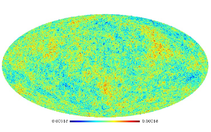
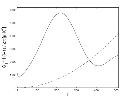
Figure 1: Properties of the maps analyzed. Left panel: Our non-Gaussian CMB signal simulation in dimensionless units. Right panel: The input signal (solid line) and noise (dashed line) power spectra.

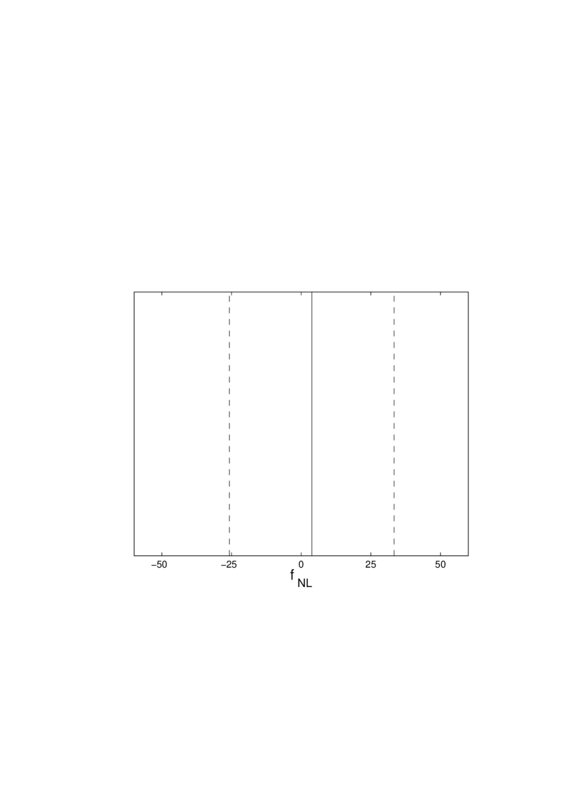
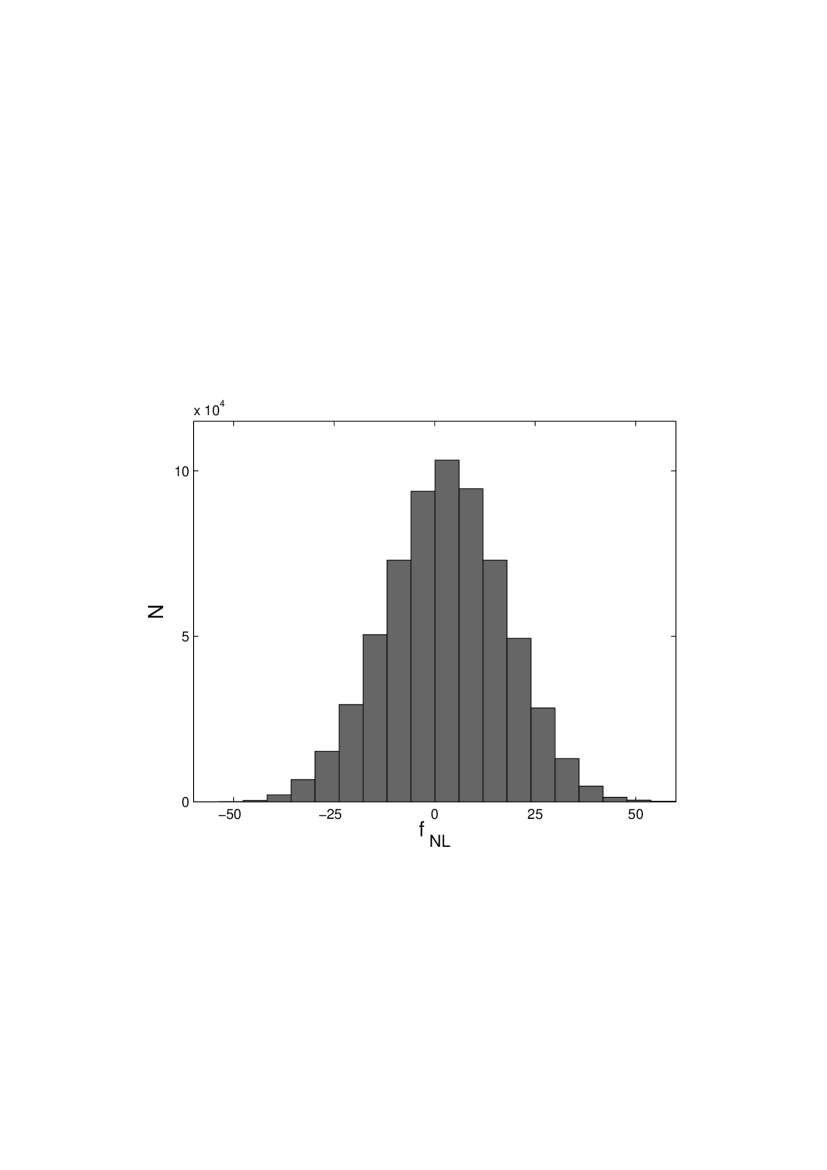
Figure 2: Analysis of the Gaussian simulation ($f_{{\mathrm{NL}}}=0$). Left panel: We show the analysis of the Gaussian CMB map by means of the frequentist estimator. Plotted are the recovered value $\hat{f}_{{\mathrm{NL}}}=4$ (solid line) and the $2-\sigma$ error (dashed lines) as derived from Monte Carlo simulations, $\sigma_{f_{{\mathrm{NL}}}}^{MC}=15$. Right panel: The analysis of the same data set within a Bayesian framework constructs the full posterior distribution $P(f_{{\mathrm{NL}}}|d,\theta)$. We obtain a mean value of $\langle f_{{\mathrm{NL}}}\rangle=3$ and a standard deviation of $\sigma_{f_{{\mathrm{NL}}}}=15$.

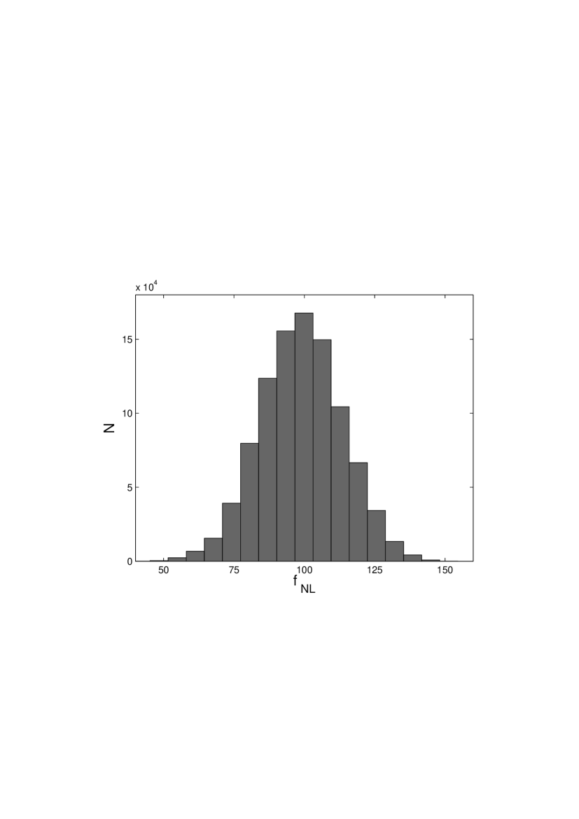
Figure 3: Same as 2, but for the non-Gaussian simulation ($f_{{\mathrm{NL}}}=100$). The results from a frequentist analysis are $\hat{f}_{{\mathrm{NL}}}=97,\ \sigma_{f_{{\mathrm{NL}}}}^{MC}=20$. Using the Bayesian method, we obtain $\langle f_{{\mathrm{NL}}}\rangle=99$ and $\sigma_{f_{{\mathrm{NL}}}}=15$. For a significant detection of $f_{{\mathrm{NL}}}$, the bispectrum estimator shows excess variance, whereas the analysis on the basis of the exact Bayesian approach still provides tight error bounds.

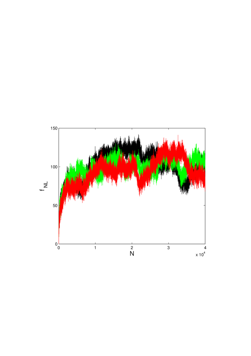
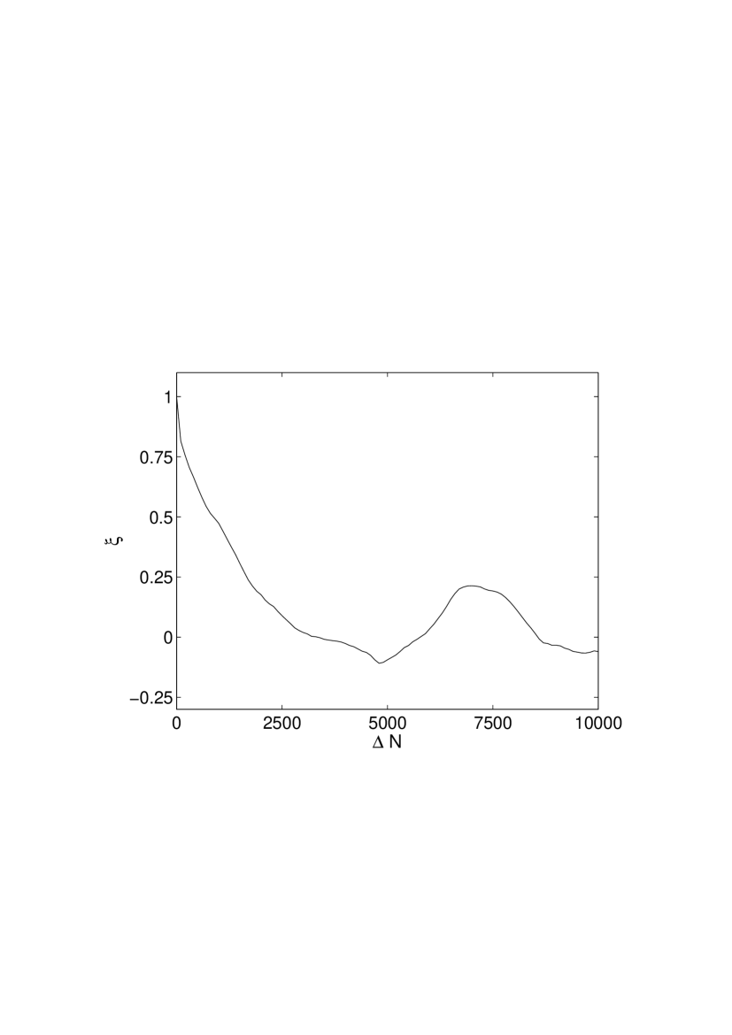
Figure 4: Performance of the sampling algorithm. Left panel: We plot a random selection of three of the 32 $f_{{\mathrm{NL}}}$ sampling chains that build up the histogram in 3. We discarded the first $10\,000$ samples during burn-in. Right panel: The autocorrelation function of a sampling chain.

5 Application to more realistic simulations

In the previous section, we have demonstrated the Bayesian approach under idealized conditions such as isotropic noise properties and a full sky analysis. However, applying the method to a realistic CMB data set requires the ability to deal with spatially varying noise properties and partial sky coverage.

In this context, a general problem is the mixture of preferred basis representations. Whereas the covariance matrix of the primordial perturbations can naturally be expressed in spherical harmonic space, the noise covariance matrix and the sky mask are defined best in pixel space. For the frequentist estimator, this is known to be problematic as e.g. in the calculation of the auxiliary map $B(r,\hat{n})$ in Eq. 5 (the Wiener filtered primordial fluctuations, see also Eqs. 3.2 for an equivalent, but more didactic expression), the inversion of a combination of the two covariance matrices has to be computed. For anisotropic noise, this can only be done by means of iterative solvers, whose numerical efficiencies depend crucially on the ability to identify powerful preconditioners.

For the Bayesian analysis scheme as presented here, however, the relevant equations do not contain any terms of this structure. Therefore, the computations remain straightforward even in the presence of arbitrary anisotropic noise properties and sky cuts. To demonstrate this ability, we performed a reanalysis of the simulated non-Gaussian temperature map of Sect. 4, now superimposed by anisotropic noise as typically expected for a high frequency WMAP channel. With these parameters, the average noise power spectrum roughly remains at a level of about $\mathcal{C}^{noise}_{\ell}\approx 10^{-7}\mathrm{mK}^{2}$, but the noise is no longer spatially invariant. Including the KQ75y7 extended temperature mask, we show the diagonal elements of the inverse noise covariance matrix in 5.

Again, for the analysis, we generated 32 independent Monte Carlo chains with $140\,000$ samples. After discarding the first $15\,000$ elements during burn-in, we applied the Gelman-Rubin convergence diagnostics to the chains and obtain a value of $R=1.5$. The computed mean of $\langle f_{{\mathrm{NL}}}\rangle=90$ and the 1-$\sigma$ error of $\sigma_{f_{{\mathrm{NL}}}}=17$ are in agreement with the input values of the simulation. We show the constructed histogram on the right hand panel of 5, demonstrating the applicability of the algorithm to realistic data sets.

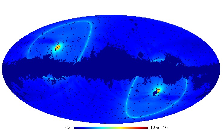
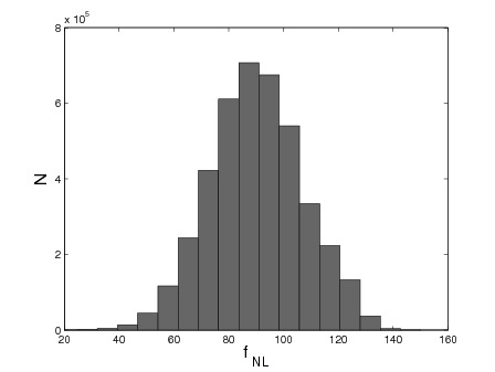
Figure 5: Analysis in case of a realistic CMB experiment. Left panel: We show the diagonal elements of the inverse noise covariance matrix in dimensionless units adopted for the more realistic simulation. When expressed in real space basis, off-diagonal terms vanish exactly. Pixel within the KQ75y7 mask are set to zero, corresponding to assigning infinite variance to them. Right panel: The constructed posterior distribution $P(f_{{\mathrm{NL}}}|d,\theta)$ of the simulated map. Obtaining $\langle f_{{\mathrm{NL}}}\rangle=90$ and $\sigma_{f_{{\mathrm{NL}}}}=17$ for the mean and standard deviation, respectively, the input value ($f_{{\mathrm{NL}}}=100$) gets consistently recovered.

6 Summary

In this paper, we introduced an exact Bayesian approach to infer the level of non-Gaussianity of local type, $f_{{\mathrm{NL}}}$, from realistic CMB temperature maps. We derived conditional probabilities for the primordial perturbations given the data, $P(\Phi_{{\mathrm{L}}}|d,\theta)$, and for $f_{{\mathrm{NL}}}$ given the data and the perturbations, $P(f_{{\mathrm{NL}}}|d,\Phi_{{\mathrm{L}}},\theta)$. We used Hamiltonian Monte Carlo sampling to draw valid realizations of $\Phi_{{\mathrm{L}}}$ from which we in turn sample $f_{{\mathrm{NL}}}$. After convergence these are samples from the full Bayesian posterior density of $f_{{\mathrm{NL}}}$ given the data.

For a direct comparison of the newly developed scheme to the conventional fast (bispectrum) estimator, we used simulated Gaussian and non-Gaussian CMB maps superimposed by isotropic noise. Estimates of the error bars within the frequentist approach were derived from Monte Carlo simulations. As a result, we find consistent outcomes between the two approaches for the analyzed Gaussian map, in agreement with the fact that the fast estimator is optimal in the limit of vanishing non-Gaussianity. In the non-Gaussian case, however, the advantage of the exact Bayesian approach becomes important. Here, the uncertainty in $f_{{\mathrm{NL}}}$ remains at the same level as for the Gaussian simulation, whereas the frequentist technique suffers from excess variance. Our results give the first example of an estimator (the “mean posterior estimator”) that saturates the Cramer-Rao bound for $f_{{\mathrm{NL}}}$ even if the signal is detectably non-Gaussian.

Finally, we demonstrate the applicability of the newly developed method to a realistic data set with spatially varying noise properties and partial sky coverage. Considering a WMAP-like noise covariance matrix and imposing the KQ75y7 extended temperature analysis mask, we analyze a non-Gaussian simulation and recover the input value consistently.

In the limit of undetectable non-Gaussianity, the Bayesian approach ought to yield the same information as the optimal bispectrum estimator (Babich 2005; Creminelli et al. 2007). Even in that limit it is useful as a cross-check since it is implemented in a completely different way. Although being computationally expensive, we conclude that the method presented here is a viable tool to exactly infer the level of non-Gaussianity of local type from CMB radiation experiments within a Bayesian framework.

References

- Acquaviva et al. (2003) Acquaviva, V., Bartolo, N., Matarrese, S., & Riotto, A. 2003, Nuclear Physics B, 667, 119
- Albrecht & Steinhardt (1982) Albrecht, A. & Steinhardt, P. J. 1982, Physical Review Letters, 48, 1220
- Babich (2005) Babich, D. 2005, Phys. Rev. D, 72, 043003
- Barreiro et al. (2004) Barreiro, R. B., Hobson, M. P., Banday, A. J., et al. 2004, MNRAS, 351, 515
- Creminelli et al. (2006) Creminelli, P., Nicolis, A., Senatore, L., Tegmark, M., & Zaldarriaga, M. 2006, Journal of Cosmology and Astro-Particle Physics, 5, 4
- Creminelli et al. (2007) Creminelli, P., Senatore, L., & Zaldarriaga, M. 2007, Journal of Cosmology and Astro-Particle Physics, 3, 19
- Dickinson et al. (2009) Dickinson, C., Eriksen, H. K., Banday, A. J., et al. 2009, ApJ, 705, 1607
- Duane et al. (1987) Duane, S., Kennedy, A. D., J., P. B., & D., R. 1987, Physics Letters B, 195, 216
- Efstathiou et al. (2009) Efstathiou, G., Ma, Y., & Hanson, D. 2009, ArXiv e-prints
- Elsner & Wandelt (2009) Elsner, F. & Wandelt, B. D. 2009, ApJS, 184, 264
- Elsner et al. (2010) Elsner, F., Wandelt, B. D., & Schneider, M. D. 2010, A&A, 513, A59+
- Enqvist & Sloth (2002) Enqvist, K. & Sloth, M. S. 2002, Nuclear Physics B, 626, 395
- Enßlin et al. (2009) Enßlin, T. A., Frommert, M., & Kitaura, F. S. 2009, Phys. Rev. D, 80, 105005
- Eriksen et al. (2008a) Eriksen, H. K., Dickinson, C., Jewell, J. B., et al. 2008a, ApJ, 672, L87
- Eriksen et al. (2006) Eriksen, H. K., Dickinson, C., Lawrence, C. R., et al. 2006, New Astronomy Review, 50, 861
- Eriksen et al. (2008b) Eriksen, H. K., Jewell, J. B., Dickinson, C., et al. 2008b, ApJ, 676, 10
- Gangui et al. (1994) Gangui, A., Lucchin, F., Matarrese, S., & Mollerach, S. 1994, ApJ, 430, 447
- Gelman & Rubin (1992) Gelman, A. & Rubin, D. B. 1992, Statistical Science, 7, 457
- Górski et al. (2005) Górski, K. M., Hivon, E., Banday, A. J., et al. 2005, ApJ, 622, 759
- Guth (1981) Guth, A. H. 1981, Phys. Rev. D, 23, 347
- Hinshaw et al. (2009) Hinshaw, G., Weiland, J. L., Hill, R. S., et al. 2009, ApJS, 180, 225
- Hobson et al. (1998) Hobson, M. P., Jones, A. W., Lasenby, A. N., & Bouchet, F. R. 1998, MNRAS, 300, 1
- Jewell et al. (2004) Jewell, J., Levin, S., & Anderson, C. H. 2004, ApJ, 609, 1
- Jewell et al. (2009) Jewell, J. B., Eriksen, H. K., Wandelt, B. D., et al. 2009, ApJ, 697, 258
- Khoury et al. (2001) Khoury, J., Ovrut, B. A., Steinhardt, P. J., & Turok, N. 2001, Phys. Rev. D, 64, 123522
- Komatsu et al. (2009) Komatsu, E., Dunkley, J., Nolta, M. R., et al. 2009, ApJS, 180, 330
- Komatsu et al. (2003) Komatsu, E., Kogut, A., Nolta, M. R., et al. 2003, ApJS, 148, 119
- Komatsu et al. (2010) Komatsu, E., Smith, K. M., Dunkley, J., et al. 2010, ArXiv e-prints
- Komatsu et al. (2005) Komatsu, E., Spergel, D. N., & Wandelt, B. D. 2005, ApJ, 634, 14
- Komatsu et al. (2002) Komatsu, E., Wandelt, B. D., Spergel, D. N., Banday, A. J., & Górski, K. M. 2002, ApJ, 566, 19
- Larson et al. (2010) Larson, D., Dunkley, J., Hinshaw, G., et al. 2010, ArXiv e-prints
- Larson et al. (2007) Larson, D. L., Eriksen, H. K., Wandelt, B. D., et al. 2007, ApJ, 656, 653
- Liguori et al. (2003) Liguori, M., Matarrese, S., & Moscardini, L. 2003, ApJ, 597, 57
- Liguori et al. (2007) Liguori, M., Yadav, A., Hansen, F. K., et al. 2007, Phys. Rev. D, 76, 105016
- Linde (1982) Linde, A. D. 1982, Physics Letters B, 108, 389
- Lyth et al. (2003) Lyth, D. H., Ungarelli, C., & Wands, D. 2003, Phys. Rev. D, 67, 023503
- Maldacena (2003) Maldacena, J. 2003, Journal of High Energy Physics, 5, 13
- Moroi & Takahashi (2001) Moroi, T. & Takahashi, T. 2001, Physics Letters B, 522, 215
- Pitrou et al. (2010) Pitrou, C., Uzan, J., & Bernardeau, F. 2010, ArXiv e-prints
- Rocha et al. (2001) Rocha, G., Magueijo, J., Hobson, M., & Lasenby, A. 2001, Phys. Rev. D, 64, 063512
- Salopek & Bond (1990) Salopek, D. S. & Bond, J. R. 1990, Phys. Rev. D, 42, 3936
- Smith et al. (2009) Smith, K. M., Senatore, L., & Zaldarriaga, M. 2009, Journal of Cosmology and Astro-Particle Physics, 9, 6
- Smith et al. (2007) Smith, K. M., Zahn, O., & Doré, O. 2007, Phys. Rev. D, 76, 043510
- Spergel et al. (2007) Spergel, D. N., Bean, R., Doré, O., et al. 2007, ApJS, 170, 377
- Spergel et al. (2003) Spergel, D. N., Verde, L., Peiris, H. V., et al. 2003, ApJS, 148, 175
- Starobinskiǐ (1982) Starobinskiǐ, A. A. 1982, Physics Letters B, 117, 175
- Steinhardt & Turok (2002) Steinhardt, P. J. & Turok, N. 2002, Phys. Rev. D, 65, 126003
- Taylor et al. (2008) Taylor, J. F., Ashdown, M. A. J., & Hobson, M. P. 2008, MNRAS, 389, 1284
- Vielva & Sanz (2009) Vielva, P. & Sanz, J. L. 2009, MNRAS, 397, 837
- Wandelt et al. (2004) Wandelt, B. D., Larson, D. L., & Lakshminarayanan, A. 2004, Phys. Rev. D, 70, 083511
- Yadav et al. (2007) Yadav, A. P. S., Komatsu, E., & Wandelt, B. D. 2007, ApJ, 664, 680
- Yadav et al. (2008) Yadav, A. P. S., Komatsu, E., Wandelt, B. D., et al. 2008, ApJ, 678, 578
- Yadav & Wandelt (2008) Yadav, A. P. S. & Wandelt, B. D. 2008, Physical Review Letters, 100, 181301
- Yadav & Wandelt (2010) Yadav, A. P. S. & Wandelt, B. D. 2010, ArXiv e-prints