Reynolds stress and heat flux in spherical shell convection

Abstract

Context. Turbulent fluxes of angular momentum and enthalpy or heat due to rotationally affected convection play a key role in determining differential rotation of stars. Their dependence on latitude and depth has been determined in the past from convection simulations in Cartesian or spherical simulations. Here we perform a systematic comparison between the two geometries as a function of the rotation rate.

Aims. Here we want to extend the earlier studies by using spherical wedges to obtain turbulent angular momentum and heat transport as functions of the rotation rate from stratified convection. We compare results from spherical and Cartesian models in the same parameter regime in order to study whether restricted geometry introduces artefacts into the results. In particular, we want to clarify whether the sharp equatorial profile of the horizontal Reynolds stress found in earlier Cartesian models is also reproduced in spherical geometry.

Methods. We employ direct numerical simulations of turbulent convection in spherical and Cartesian geometries. In order to alleviate the computational cost in the spherical runs, and to reach as high spatial resolution as possible, we model only parts of the latitude and longitude. The rotational influence, measured by the Coriolis number or inverse Rossby number, is varied from zero to roughly seven, which is the regime that is likely to be realised in the solar convection zone. Cartesian simulations are performed in overlapping parameter regimes.

Results. For slow rotation we find that the radial and latitudinal turbulent angular momentum fluxes are directed inward and equatorward, respectively. In the rapid rotation regime the radial flux changes sign in accordance with earlier numerical results, but in contradiction with theory. The latitudinal flux remains mostly equatorward and develops a maximum close to the equator. In Cartesian simulations this peak can be explained by the strong ‘banana cells’. Their effect in the spherical case does not appear to be as large. The latitudinal heat flux is mostly equatorward for slow rotation but changes sign for rapid rotation. Longitudinal heat flux is always in the retrograde direction. The rotation profiles vary from anti-solar (slow equator) for slow and intermediate rotation to solar-like (fast equator) for rapid rotation. The solar-like profiles are dominated by the Taylor–Proudman balance.

1 Introduction

The surface of the Sun rotates differentially: the rotation period at the poles is roughly 35 days as opposed to 26 days at the equator. Furthermore, the internal rotation of the Sun has been revealed by helioseismology (e.g. Thompson et al. Tea03 (2003)): the radial gradient of $\Omega$ is small in the bulk of the convection zone, whereas regions of strong radial differential rotation are found near the base and near the surface of the convection zone. According to dynamo theory, large-scale shear plays an important role in generating large-scale magnetic fields (e.g., Moffatt M78 (1978); Krause & Rädler KR80 (1980)). More specifically, large-scale shear lowers the threshold for dynamo action and the combined effect of helical turbulence and shear yields oscillatory large-scale magnetic fields, resembling the observed solar activity pattern (e.g. Yoshimura Y75 (1975)). It is even possible to drive a large-scale dynamo in nonhelical turbulence with shear (e.g., Brandenburg B05 (2005); Yousef et al. 2008a ; 2008b ; Brandenburg et al. BRRK08 (2008)). Thus, it is of great interest to study the processes that generate large-scale shear in solar and stellar convection zones.

Differential rotation of the Sun and other stars is thought to be maintained by rotationally influenced turbulence in their convection zones. In hydrodynamic mean-field theories of stellar interiors the effects of turbulence appear in the form of turbulent fluxes of angular momentum and enthalpy or heat (cf. Rüdiger R89 (1989); Rüdiger & Hollerbach RH04 (2004)). These fluxes can be defined by Reynolds averaging of products of fluctuating quantities, v.i.z., the fluxes of angular momentum and heat, respectively, are

$$Q_{ij} = \overline{u_{i}^{\prime}u_{j}^{\prime}},$$ (1)

$$F_{i} = c_{\rm P}\overline{\rho}\;\overline{u_{i}^{\prime}T^{\prime}}.$$ (2)

Here overbars denote azimuthal averaging, primes denote fluctuations about the averages, $Q_{ij}$ is the Reynolds stress, $F_{i}$ is the turbulent convective energy flux, $\bm{u}$ is the velocity, $T$ is the temperature, $\rho$ is density, and $c_{\rm P}$ is the specific heat at constant pressure.

Much effort has been put into computing these correlations using analytical theories (e.g., Rüdiger R80 (1980, 1982); Kitchatinov & Rüdiger KR93 (1993); Kitchatinov et al. KPR94 (1994)). Most of the analytical studies, however, rely on approximations such as first-order smoothing, the applicability of which in the stellar environments can be contested. In order to get more insight, idealised numerical simulations, often working in Cartesian geometry, have been extensively used to compute the stresses for modestly large Reynolds numbers (e.g., Pulkkinen et al. Pea93 (1993); Brummell et al. BHT98 (1998); Chan C01 (2001); Käpylä et al. KKT04 (2004); Rüdiger et al. 2005b ). However, the Cartesian simulations have yielded some puzzling results, such as the latitudinal angular momentum flux having a very strong maximum very close to the equator (e.g., Chan C01 (2001); Hupfer et al. HKS05 (2005)) and a sign change of the corresponding radial flux (Käpylä et al. KKT04 (2004)). Neither of these effects can be recovered from theoretical studies (Rüdiger & Hollerbach RH04 (2004)) or simpler forced turbulence simulations (Käpylä & Brandenburg KB08 (2008)). The Reynolds stresses have also been computed from high resolution spherical convection simulations (e.g. DeRosa et al. DGT02 (2002); Miesch et al. MBDRT08 (2008)), but a detailed comparison with Cartesian results is lacking in the literature.

Rotation also affects the turbulent convective energy transport. In fact, in the presence of rotation, the turbulent heat transport due to convection is no longer purely radial (e.g., Brandenburg et al. BMT92 (1992); Kitchatinov et al. KPR94 (1994); Brun & Rempel BR09 (2009)). In a sphere, such anisotropic heat transport leads to latitude-dependent temperature and entropy distributions. Such variations can be important in determining the rotation profile of the Sun: neglecting the Reynolds stress and molecular diffusion, the evolution of the azimuthal component of vorticity, $\overline{\bm{\omega}}=\bm{\nabla}\times\overline{\bm{u}}$, is governed by

$$\frac{\partial\overline{\omega}_{\phi}}{\partial t}=r\sin\theta\frac{\partial\overline{\Omega}^{2}}{\partial z}+\frac{1}{\overline{\rho}^{2}}(\bm{\nabla}\overline{\rho}\times\bm{\nabla}\overline{p})_{\phi},$$ (3)

where $\partial/\partial z=\hat{\mbox{\boldmath$\Omega$}}{}\cdot\mbox{\boldmath$\nabla$}{}$ is the derivative along the unit vector of the rotation vector, $\hat{\mbox{\boldmath$\Omega$}}{}=(\cos\theta,-\sin\theta,0)$, and $p$ is the pressure. The last term on the rhs describes the baroclinic term which can be written as

$$\frac{1}{\overline{\rho}^{2}}(\bm{\nabla}\overline{\rho}\times\bm{\nabla}\overline{p})_{\phi}=(\bm{\nabla}\overline{T}\times\bm{\nabla}\overline{s})_{\phi}\approx-\frac{g}{rc_{\rm P}}\frac{\partial\overline{s}}{\partial\theta}.$$ (4)

where $g=|\@vec{g}|$ is the acceleration due to gravity, $s$ is the specific entropy, and $\bm{\nabla}\overline{T}\approx\@vec{g}/c_{\rm P}$ has been used for the adiabatic temperature gradient. In the absence of latitudinal entropy gradients, the solution of Eq. (3) is given by the Taylor–Proudman theorem, i.e. $\partial\overline{\Omega}/\partial z=0$. In general, however, the thermodynamics cannot be neglected and latitudinal gradients of entropy influence the rotation profile of the star via the baroclinic term. Such an effect is widely considered to be instrumental in breaking the Taylor–Proudman balance in the solar case (e.g., Rempel R05 (2005); Miesch et al. MBT06 (2006)). Local simulations can be used to determine the latitudinal heat flux but by virtue of periodic boundaries, no information about the latitudinal profile of entropy can be extracted from a single simulation. Earlier local studies suggest that in the presence of rotation the latitudinal heat flux is directed towards the poles (e.g. Rüdiger et al. 2005b ) and mean-field models in spherical geometry indicate that such a flux leads to warm poles and a cooler equator (e.g. Brandenburg et al. BMT92 (1992)), thus alleviating the Taylor–Proudman balance. Computing the turbulent heat fluxes in spherical geometry in order to compare with earlier results is one of the principal aims of the present study. Of particular importance is the sign and magnitude of the latitudinal heat flux.

It is possible that the use of Cartesian geometry and periodic boundaries give rise to artefacts which are not present in fully spherical geometry. In the present paper we undertake the computation of Reynolds stress and turbulent heat transport from simulations in spherical geometry as functions of rotation, and compare them with Cartesian simulations of the same system located at different latitudes. One of the most important goals of the paper is to find out whether the present results in Cartesian geometry compare with early similar studies and to test if these results are still valid when spherical geometry is used. Earlier studies comparing spherical and Cartesian models used limited two-dimensional geometry in the spherical case Hupfer et. al (HKS06 (2006)) whereas we perform all our simulations in three dimensions. Furthermore, Robinson & Chan (RC01 (2001)) used spherical wedges to compute the rotation profiles and turbulent fluxes using two representative runs. Here we explore a significantly larger portion of parameter space. As a side result we also obtain angular velocity profiles as a function of rotation from our spherical simulations which, however, are dominated by the Taylor-Proudman balance in the regime most relevant to the Sun. Thus we fail in reproducing the solar rotation profile which is a common problem that can currently be overcome only by introducing some additional poorly constrained terms, e.g. a latitudinal entropy gradient, by hand rather than self-consistently (e.g. Miesch et al. 2006). Another important use for the results will be the more ambitious future runs where subgrid-scale models of the turbulent effects can be used to overcome the Taylor–Proudman balance.

2 Model

Our spherical model is similar to that used by Käpylä et al. (2010a ) but without magnetic fields. We model a segment of a star, i.e. a “wedge”, in spherical polar coordinates where $(r,\theta,\phi)$ denote the radius, colatitude, and longitude. The radial, latitudinal, and longitudinal extents of the computational domain are given by $0.65R\leq r\leq R$, $\theta_{0}\leq\theta\leq 180\degr-\theta_{0}$, and $0\leq\phi\leq\phi_{0}$, respectively, where $R$ is the radius of the star. In all of our runs we take $\theta_{0}=15\degr$ and $\phi_{0}=90\degr$. We study the dependence of the results on domain size in Appendix A. In our Cartesian runs, the coordinates $(x,y,z)$ correspond to radius, latitude and longitude of a box located at a colatitude $\theta$. Our domain spans from $0.65R\leq x\leq R$, $-0.35R\leq y\leq 0.35R$ and $-0.35R\leq z\leq 0.35R$, i.e., the extension of the horizontal directions is twice the vertical one, as has been used in previous Cartesian simulations (e.g. Käpylä et al. KKT04 (2004)).

In both geometries, we solve the following equations of compressible hydrodynamics,

$$\frac{D\ln\rho}{Dt}=-\bm{\nabla}\cdot\bm{u},$$ (5)

$$\frac{D\bm{u}}{Dt}=\bm{g}-2\bm{\Omega}\times\bm{u}+\frac{1}{\rho}\left(\bm{\nabla}\cdot 2\nu\rho\bm{\mathsf{S}}-\bm{\nabla}p\right),$$ (6)

$$\frac{Ds}{Dt}=\frac{1}{\rho T}\left(\bm{\nabla}\cdot K\bm{\nabla}T+2\nu\bm{\mathsf{S}}^{2}-\Gamma_{\rm cool}\right),$$ (7)

where $D/Dt=\partial/\partial t+\bm{u}\cdot\bm{\nabla}$ is the advective time derivative, $\nu$ is the kinematic viscosity, $K$ is the radiative heat conductivity, and $\bm{g}$ is the gravitational acceleration given by

$$\bm{g}=-\frac{GM}{r^{2}}\hat{\bm{r}},$$ (8)

where $G$ is the gravitational constant, $M$ is the mass of the star, and $\hat{\bm{r}}$ is the unit vector in the radial direction. Note that in the Cartesian case $x$ corresponds to the $r$ direction so that all radial profiles in spherical coordinates directly apply to the Cartesian model. We omit the centrifugal force in our models. This is connected with the fact that the Rayleigh number is much less than in the Sun, which is unavoidable and constrained by the numerical resolution available. This implies that the Mach number is larger than in the Sun. Nevertheless, it is essential to have realistic Coriolis numbers. i.e. the Coriolis force has to be larger by the same amount that the turbulent velocity is larger, but without significantly altering the hydrostatic balance that is determined by gravity and centrifugal forces.

The fluid obeys the ideal gas law with $p=(\gamma-1)\rho e$, where $\gamma=c_{\rm P}/c_{\rm V}=5/3$ is the ratio of specific heats in constant pressure and volume, respectively, and $e=c_{\rm V}T$ is the internal energy. The rate of strain tensor $\bm{\mathsf{S}}$ is given by

$$\mathsf{S}_{ij}={\textstyle{1\over 2}}(u_{i;j}+u_{j;i})-{\textstyle{1\over 3}}\delta_{ij}\bm{\nabla}\cdot\bm{u},$$ (9)

where the semicolons denote covariant differentiation (see Mitra et al. MTBM09 (2009) for details).

The computational domain is divided into three parts: a lower convectively stable layer at the base, convectively unstable layer and a cooling layer at the top mimicking the effects of radiative losses at the stellar surface. The radial positions $(r_{1},r_{2},r_{3},r_{4})=(x_{1},x_{2},x_{3},x_{4})=(0.65,0.7,0.98,1)R$ give the locations of the bottom of the domain, bottom and top of the convectively unstable layer, and the top of the domain, respectively. The last term on the rhs of Eq. (7) describes cooling in the surface layer given by

$$\Gamma_{\rm cool}=\Gamma_{0}f(r)\left(\frac{c_{\rm s}^{2}-c_{\rm s0}^{2}}{c_{\rm s0}^{2}}\right),$$ (10)

where $f(r)$ is a profile function equal to unity in $r>r_{3}$ and smoothly connecting to zero below, and $\Gamma_{0}$ is a cooling luminosity chosen so that the sound speed in the uppermost layer relaxes toward $c_{\rm s0}^{2}=c_{\rm s}^{2}(r=r_{4})$.

2.1 Initial and boundary conditions

For the thermal stratification we adopt a simple setup that can be described analytically rather than adopting profiles from a solar or stellar structure model as in, e.g., Brun et al. (BMT04 (2004)). We use a piecewise polytropic setup which divides the domain into three layers. The hydrostatic temperature gradient is given by

$$\frac{\partial T}{\partial r}=\frac{-g}{c_{\rm V}(\gamma-1)(n+1)},$$ (11)

where $n=n(r)$ is the radially varying polytropic index. This gives the logarithmic temperature gradient $\nabla$ (not to be confused with the operator $\bm{\nabla}$) as

$$\nabla=\partial\ln T/\partial\ln p=(n+1)^{-1}.$$ (12)

The stratification is unstable if $\nabla-\nabla_{\rm ad}>0$ where $\nabla_{\rm ad}=1-1/\gamma$, corresponding to $n<1.5$. We choose $n=6$ for the lower overshoot layer, whereas $n=1$ is used in the convectively unstable layer. A polytropic setup with $n=1$ is commonly used in convection studies (e.g. Hurlburt et al. HTM84 (1984)). This implies that about 80 per cent of the energy is transported by radiation (cf. Brandenburg et al. BCNS05 (2005)), regardless of the vigor of convection and the value of the Reynolds number.

Density stratification is obtained by requiring hydrostatic equilibrium. The thermal conductivity is obtained by requiring a constant luminosity $L_{0}$ throughout the domain via

$$K=\frac{L_{0}}{4\pi r^{2}\partial T/\partial r}.$$ (13)

In order to expedite the initial transient due to thermal relaxation, the thermal variables have a shallower profile, corresponding to $\rho\propto T^{1.4}$, in the convection zone and $n=1$ is only used for the thermal conductivity. This gives approximately the right entropy jump that corresponds to the required flux (cf. Brandenburg et al. BCNS05 (2005)). In Fig. 1 we show the initial and final stratifications of specific entropy, temperature, density, and pressure for a particular run.

In the spherical models the radial and latitudinal boundaries are taken to be impenetrable and stress free, according to

$$u_{r}=0,\quad\frac{\partial u_{\theta}}{\partial r}=\frac{u_{\theta}}{r},\quad\frac{\partial u_{\phi}}{\partial r}=\frac{u_{\phi}}{r}\quad(r=r_{1},r_{4}),$$ (14)

$$\frac{\partial u_{r}}{\partial\theta}=u_{\theta}=0,\quad\frac{\partial u_{\phi}}{\partial\theta}=u_{\phi}\cot\theta\quad(\theta=\theta_{0},\pi-\theta_{0}).$$ (15)

On the latitudinal boundaries we assume that the thermodynamic quantities have zero first derivative, thus suppressing heat fluxes through the boundary.

In Cartesian coordinates we use periodic boundary conditions in the horizontal directions ($y$ and $z$), and stress free conditions in the $x$ direction, i.e.,

$$u_{x}=\frac{\partial u_{y}}{\partial x}=\frac{\partial u_{z}}{\partial x}=0\quad(x=x_{1},x_{4}).$$ (16)

The simulations were performed using the Pencil Code, which uses sixth-order explicit finite differences in space and a third-order accurate time stepping method (see Mitra et al. MTBM09 (2009) for further information regarding the adaptation of the Pencil Code to spherical coordinates).

Table 1: Summary of the spherical runs.

$$\begin{array}[]{p{0.05\linewidth}cccccccccccc}\hline\cr\vskip 3.0pt plus 1.0pt minus 1.0pt\cr Run&$grid$&{\rm Ra}&{\rm Pr}&\mathcal{L}&{\rm Ma}&{\rm Re}&{\rm Co}&\tilde{E}_{\rm ther}&\tilde{E}_{\rm kin}&E_{\rm mer}/E_{\rm kin}&E_{\rm rot}/E_{\rm kin}&\Delta\Omega/\Omega_{\rm eq}\\ \hline\cr A0&128\times 256\times 128&3.1\cdot 10^{6}&1.0&1.4\cdot 10^{-4}&0.023&38&0.00&0.116&7.7\cdot 10^{-5}&0.045&0.004&-\\ \hline\cr A1&128\times 256\times 128&3.1\cdot 10^{6}&1.0&1.4\cdot 10^{-4}&0.022&36&0.13&0.114&6.9\cdot 10^{-5}&0.016&0.022&-0.15\\ A2&128\times 256\times 128&3.1\cdot 10^{6}&1.0&1.4\cdot 10^{-4}&0.022&36&0.25&0.114&7.2\cdot 10^{-5}&0.015&0.073&-0.31\\ A3&128\times 256\times 128&3.1\cdot 10^{6}&1.0&1.4\cdot 10^{-4}&0.022&37&0.50&0.113&1.2\cdot 10^{-4}&0.010&0.438&-1.03\\ A4&128\times 256\times 128&3.1\cdot 10^{6}&1.0&1.4\cdot 10^{-4}&0.029&48&0.94&0.112&1.1\cdot 10^{-3}&0.016&0.927&-1.74\\ A5&128\times 256\times 128&3.1\cdot 10^{6}&1.0&1.4\cdot 10^{-4}&0.022&36&2.56&0.111&9.9\cdot 10^{-4}&0.002&0.949&-0.37\\ A6&128\times 256\times 128&3.1\cdot 10^{6}&1.0&1.4\cdot 10^{-4}&0.018&30&6.09&0.114&2.3\cdot 10^{-4}&0.000&0.824&+0.20\\ \hline\cr B0&128\times 512\times 256&8.6\cdot 10^{6}&1.0&1.4\cdot 10^{-4}&0.020&54&0.00&0.113&5.8\cdot 10^{-5}&0.036&0.009&-\\ \hline\cr B1&128\times 512\times 256&8.6\cdot 10^{6}&1.0&1.4\cdot 10^{-4}&0.020&57&1.34&0.112&6.5\cdot 10^{-4}&0.009&0.927&-1.10\\ B2&128\times 512\times 256&8.6\cdot 10^{6}&1.0&1.4\cdot 10^{-4}&0.018&50&3.06&0.113&1.2\cdot 10^{-4}&0.001&0.689&+0.12\\ B3&128\times 512\times 256&8.6\cdot 10^{6}&1.0&1.4\cdot 10^{-4}&0.016&44&6.93&0.113&1.8\cdot 10^{-4}&0.000&0.833&+0.20\\ \hline\cr C1&128\times 256\times 128&1.7\cdot 10^{7}&6.7&7.5\cdot 10^{-5}&0.008&12&7.58&0.114&3.8\cdot 10^{-5}&0.000&0.817&+0.12\\ \hline\cr D1&256\times 512\times 256&6.0\cdot 10^{7}&1.0&3.1\cdot 10^{-5}&0.012&90&5.07&0.113&7.9\cdot 10^{-5}&0.000&0.796&+0.20\\ D2&256\times 512\times 256&6.0\cdot 10^{7}&1.0&3.1\cdot 10^{-5}&0.012&89&7.68&0.113&1.5\cdot 10^{-4}&0.000&0.895&+0.20\\ \hline\cr\end{array}$$

Figure 1: Radial profiles of entropy, temperature, density, and pressure in the initial state (solid lines) and the in the saturated state (dashed) of Run B0. Reference values $T_{0}$ and $p_{0}$ are taken from the bottom of the convectively unstable layer in the initial state. The dotted vertical lines at $r_{2}=0.7R$ and $r_{3}=0.98R$ denote the bottom and top of the convectively unstable layer, respectively.

2.2 Nondimensional quantities

Dimensionless quantities are obtained by setting

$$R=GM=\rho_{0}=c_{\rm P}=1\;,$$ (17)

where $\rho_{0}$ is the density at $r_{2}$, The units of length, velocity, density, and entropy are then given by

$$[x]=R\;,\;\;[u]=\sqrt{GM/R}\;,\;\;[\rho]=\rho_{0}\;,\;\;[s]=c_{\rm P}\;.$$ (18)

The Cartesian simulations have been arranged so that the thickness of the layers is the same, $\@vec{g}=-(GM/x^{2})\hat{\bm{x}}$, and $R$, which is still our unit length, has no longer the meaning of a radius. The simulations are governed by the Prandtl, Reynolds, Coriolis, and Rayleigh numbers, defined by

$${\rm Pr} \!=\! \frac{\nu}{\chi_{0}}\;,\;\;{\rm Re}=\frac{u_{\rm rms}}{\nu k_{\rm f}}\;,\;\;{\rm Co}=\frac{2\,\Omega_{0}}{u_{\rm rms}k_{\rm f}}\;,$$ (19)

$${\rm Ra} \!=\! \frac{GM(\Delta r)^{4}}{\nu\chi_{0}R^{2}}\bigg{(}-\frac{1}{c_{\rm P}}\frac{{\rm d}s}{{\rm d}r}\bigg{)}_{r_{\rm m}}\;,$$ (20)

where $\chi_{0}=K/(\rho_{\rm m}c_{\rm P})$ is the thermal diffusivity, $k_{\rm f}=2\pi/\Delta r$ is an estimate of the wavenumber of the energy-carrying eddies, $\Delta r=r_{3}-r_{2}$ is the thickness of the unstable layer, $\rho_{\rm m}$ is the density in the middle of the unstable layer at  $r_{\rm m}=(r_{3}+r_{2})/2$, and $u_{\rm rms}=\sqrt{{\textstyle{3\over 2}}\langle u_{r}^{2}+u_{\theta}^{2}\rangle}$ is the rms velocity, where the angular brackets denote volume averaging. In our definition of $u_{\rm rms}$ we omit the contribution from the $\phi$-component of velocity, because it is dominated by the large-scale differential rotation that develops when rotation is included. The entropy gradient, measured at $r_{\rm m}$ in the initial non-convecting state, is given by

$$\bigg{(}-\frac{1}{c_{\rm P}}\frac{{\rm d}s}{{\rm d}r}\bigg{)}_{r_{\rm m}}=\frac{\nabla_{\rm m}-\nabla_{\rm ad}}{H_{\rm P}}\;,$$ (21)

where $\nabla_{\rm m}=(\partial\ln T/\partial\ln p)_{r_{\rm m}}$, and $H_{\rm P}$ is the pressure scale height at $r_{\rm m}$.

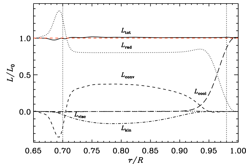
Figure 2: Radiative (dotted line), enthalpy (dashed), kinetic energy (dash-dotted), cooling (long dashed), and viscous (triple-dot-dashed) luminosities as functions of radius from Run A0. The solid line shows the sum of all fluxes, and the red dashed line the luminosity $L_{0}$ fed into the domain through the lower boundary. The vertical dotted lines at $r=0.7R$ and $r=0.98R$ denote respectively the bottom and top of the convectively unstable layer in the initial state.

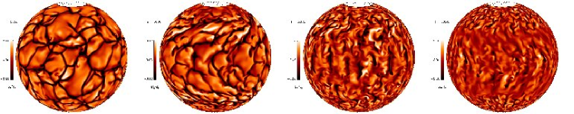
Figure 3: Radial velocity $u_{r}$ at a small distance ($r=0.9R$) below the surface from Runs B0–B3. The scales give $u_{r}$ in units of the local sound speed. For visualization purposes, the domain is duplicated fourfold in the longitudinal direction. See also http://www.helsinki.fi/$\sim$kapyla/movies.html

The energy that is deposited into the domain at the base is controlled by the luminosity parameter

$$\mathcal{L}=\frac{L_{0}}{\rho_{0}(GM)^{3/2}R^{1/2}},$$ (22)

where $L_{0}=4\pi r_{1}^{2}F_{\rm b}$ is the constant luminosity, and $F_{\rm b}=-(K\partial T/\partial r)|_{r=r_{1}}$ is the energy flux imposed at the lower boundary. Furthermore, the stratification is determined by the pressure scale height at the surface

$$\xi=\frac{(\gamma-1)c_{\rm V}T_{4}}{GM/R},$$ (23)

where $T_{4}=T(r=r_{4})$. Similar parameter definitions were used by Dobler et al. (DSB06 (2006)). We use $\xi=0.020$, which results in a density contrast of $10^{2}$ across the domain.

3 Results

Our main goal is to extract the turbulent fluxes of angular momentum and heat as functions of rotation from our simulations. In order to achieve this we use a moderately turbulent model and vary the rotation rate, quantified by the Coriolis number, from zero to roughly six in Set A (see Table 1). We also perform a subset of these simulations at higher resolution in Set B and a three runs (C1, D1, and D2) with a lower Mach number. The runs in Set A were initialized from scratch, whereas in Set B a nonrotating simulation B0 was run until it was thermally relaxed. The runs with rotation (B1–B3) were then started from this snapshot and computations carried out until a new saturated state was reached. The runs D1 and D2 were remeshed from a non-rotating, thermally relaxed model at a lower resolution. In Fig. 1 we compare the initial and final stratification of specific entropy, temperature, density, and pressure for Run B0.

As noted in Sect. 2.1, our polytropic setup leads to a system where radiative diffusion transports 80 per cent of the total energy. We show the flux balance in the statistically saturated state from Run A0 in Fig. 2, where the different contributions are given in terms of luminosities $L_{i}=4\pi r^{2}F_{i}$, and where

$$F_{\rm rad} = -K\frac{\partial T}{\partial r},$$ (24)

$$F_{\rm conv} = -c_{\rm P}\overline{\rho}\overline{u_{r}^{\prime}T^{\prime}},$$ (25)

$$F_{\rm kin} = {\textstyle{1\over 2}}\overline{\rho}\overline{u^{2}u_{r}},$$ (26)

$$F_{\rm visc} = -2\nu\overline{\rho}\ \overline{u_{i}\mathsf{S}_{ir}},$$ (27)

$$F_{\rm cool} = \int\Gamma_{\rm cool}\ dr.$$ (28)

Here we consider averages over $\phi$ and $\theta$. We find that in the non-rotating case the convective flux accounts for roughly 30 per cent of the total luminosity and the (inward) kinetic energy flux is between 10 and 15 per cent. When rotation is increased, both the convective and kinetic fluxes decrease. The viscous flux is always negligible. The cooling flux transports the total luminosity near the surface.

Visualizations of $u_{r}$ at a small distance below the surface are shown in Fig. 3 for Runs B0–B3. The convective velocities $\@vec{u}^{\prime}$ can be decomposed in terms of poloidal ($\@vec{u}^{\prime}_{\rm P}$) and toroidal ($\@vec{u}^{\prime}_{\rm T}$) parts following Lavely & Ritzwoller (LR92 (1992))

$$\@vec{u}^{\prime}_{\rm P}={\rm Real}\sum_{l,m}\left\{u_{\rm P}^{lm}(r)Y_{l}^{m}\hat{\bm{r}}+v_{\rm P}^{lm}(r)\bm{\nabla}Y_{l}^{m}\right\},$$ (29)

$$\@vec{u}^{\prime}_{\rm T}={\rm Real}\sum_{l,m}\left\{w_{\rm T}^{lm}(r)\hat{\bm{r}}\times\bm{\nabla}Y_{l}^{m}\right\},$$ (30)

where $Y_{l}^{m}(\theta,\phi)$ are spherical harmonics of degree $l$ and order $m$. The geometry and amplitude of the poloidal velocity are completely defined by $l$, $m$, and $u_{\rm P}^{lm}$ since, assuming approximate mass conservation, $v_{\rm P}^{lm}$ and $u_{\rm P}^{lm}$ are related as

$$v_{\rm P}^{lm}(r)=\frac{\partial_{r}(r^{2}\rho u_{\rm P}^{lm}(r))}{\rho rl(l+1)}.$$ (31)

The poloidal flow has characteristics of Bénard convection cells with upwellings at the centres of cells and downdraughts on the peripheries. The toroidal flows are characterised by their amplitude and geometry given by $w_{\rm T}^{lm}$, $l$, and $m$ respectively. In contrast to poloidal flows, their nature resembles that of rotation, jets or horizontal vortices. In Fig. 3, we observe that so called banana cells become prominent in the radial velocity with an increase in the Coriolis number. Such structures are poloidal flows given by spherical harmonic $Y_{l}^{m}(\theta,\phi)$. For Run B3 in Fig. 3, we find maximum power at $m=16$. Note that the reality of the banana cells in the Sun is hotly debated. Even though significant power is found at wavenumbers corresponding to giant cells in the surface velocity spectra of the Sun, no distinct peak has been found at those wavenumbers (Chou et al. Cea91 (1991); Hathaway et al. Hea00 (2000)). Global helioseismology caps the maximum radial velocity of the banana cells at $50$ m s^-1 (Chatterjee & Antia CA09 (2009)). We study the importance of the banana cells to the Reynolds stresses in more detail in Sects. 3.1 and 3.2.1.

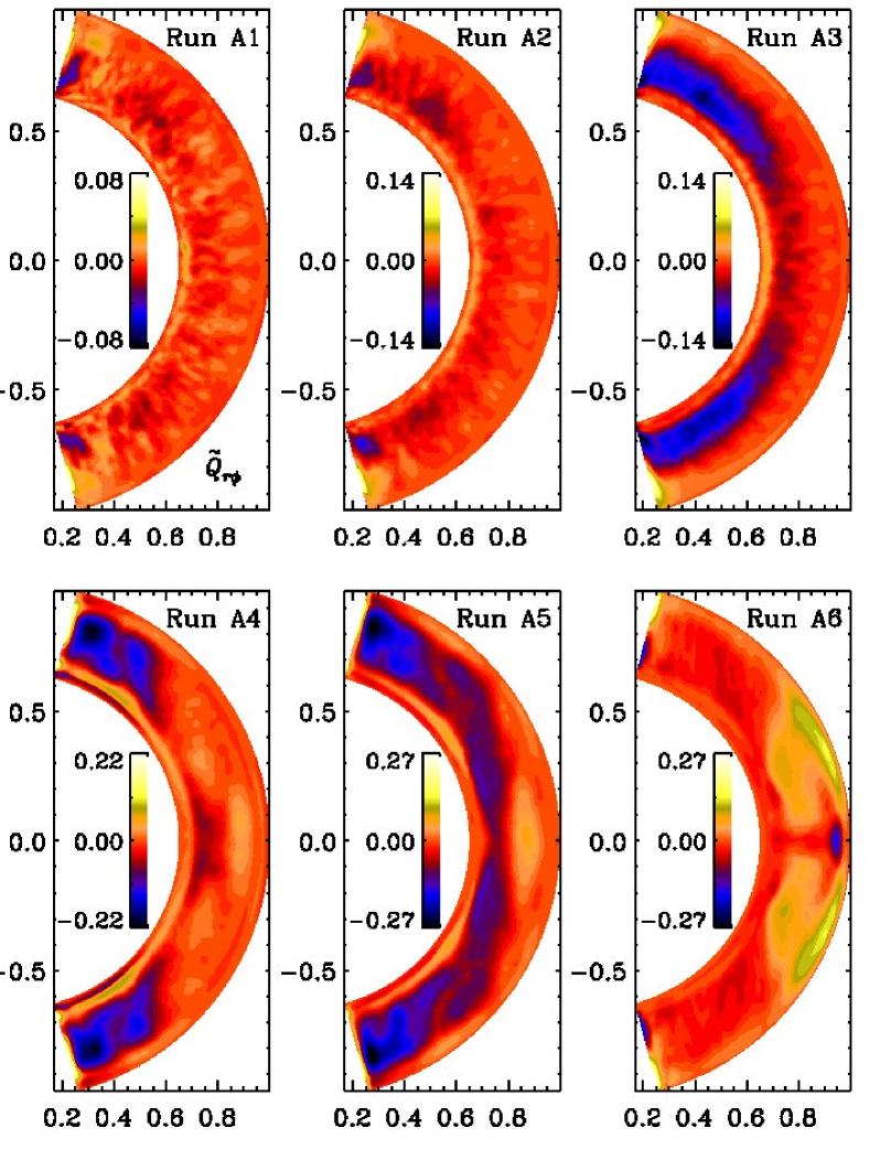
Figure 4: Vertical Reynolds stress, $\tilde{Q}_{r\phi}$, from Set A.

3.1 Reynolds stress

The angular momentum balance of a star is governed by the conservation law (Rüdiger R89 (1989))

$$\frac{\partial}{\partial t}(\overline{\rho}\varpi^{2}\overline{\Omega})=-\bm{\nabla}\cdot\left[\overline{\rho}\varpi\left(\varpi\overline{\Omega}\overline{\bm{u}}_{\rm mer}+\overline{u_{\phi}^{\prime}\bm{u}^{\prime}}\right)\right],$$ (32)

where $\varpi=r\sin\theta$ is the lever arm and $\overline{\bm{u}}_{\rm mer}=(\overline{u}_{r},\overline{u}_{\theta})$ is the meridional circulation. The latter term on the rhs describes the effects of the Reynolds stress components $Q_{r\phi}$ and $Q_{\theta\phi}$, which describe radial and latitudinal fluxes of angular momentum, respectively. The stress is often parameterised by turbulent transport coefficients that couple small-scale correlations with large-scale quantities, i.e.

$$Q_{ij}=\Lambda_{ijk}\overline{\Omega}_{k}-\mathcal{N}_{ijkl}\frac{\partial\overline{u}_{k}}{\partial x_{l}},$$ (33)

where $\Lambda_{ijk}$ describes the nondiffusive contribution ($\Lambda$-effect) and $\mathcal{N}_{ijkl}$ the diffusive part (turbulent viscosity), cf. Rüdiger (R89 (1989)). However, disentangling the two contributions is not possible, see e.g., Snellman et al. (SKKL09 (2009)) and Käpylä et al. (2010b ). We postpone a detailed study of the turbulent transport coefficients to a future study and concentrate on comparing the total stress with simulations in Cartesian geometry.

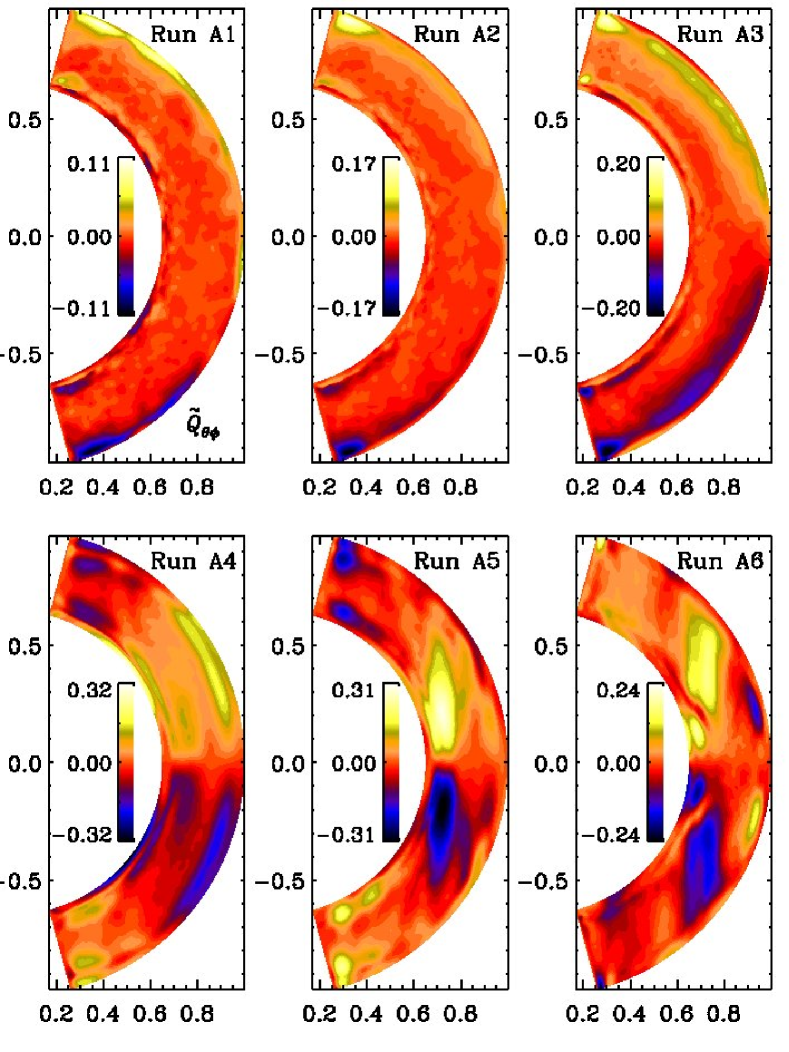
Figure 5: Horizontal Reynolds stress, $\tilde{Q}_{\theta\phi}$, from Set A.

It is convenient to display the components of the Reynolds stress in non-dimensional form (indicated by a tilde), and to define

$$\tilde{Q}_{ij}=\overline{u_{i}^{\prime}u^{\prime}_{j}}/u_{\rm rms}^{2},$$ (34)

where $u_{\rm rms}=u_{\rm rms}(r,\theta)$ is the meridional rms-velocity. The averages are calculated over the azimuthal direction and time also for $u_{\rm rms}$. In the following, we refer to the three off-diagonal components, $Q_{r\phi}$, $Q_{\theta\phi}$, and $Q_{r\theta}$, as vertical, horizontal, and meridional components, respectively. Representative results for the vertical stress component $Q_{r\phi}$ are shown in Fig. 4. We find that for slow rotation (Run A1), $Q_{r\phi}$ is small and does not appear to show a clear trend in latitude. In Run A2 with ${\rm Co}\approx 0.25$ the stress is more consistently negative within the convectively unstable layer, showing a symmetric profile with respect to the equator. These two runs tend to show the largest signal near the latitudinal boundaries which is most likely due to the boundary conditions there. Similar distortions are also seen in the large-scale flows (see Sect. 3.4). In the intermediate rotation regime (Runs A3–A5), $Q_{r\phi}$ is predominantly negative, although regions of opposite sign start to appear near the equator. In Run A6 the stress is mostly positive. Qualitatively similar results are obtained from the runs in Set B, Runs C1, D1, and D2. Therefore there is a sign change roughly at ${\rm Co}=2$. The results for most quantities from Runs B2 and D1 with intermediate values of ${\rm Co}$ are similar to those of Runs A5 and A6, respectively. Thus, we usually show results only from Runs A4, A5, and A6 in order to demonstrate the qualitative change that occurs for many quantities in the range ${\rm Co}\approx 1\ldots 6$. A similar phenomenon has been observed in Cartesian simulations (Käpylä et al. KKT04 (2004)). We note that the behaviour of $Q_{r\phi}$ in the most rapidly rotating runs, namely a small negative region at the equator and a positive peak near the surface at somewhat higher latitudes was also reported by Robinson & Chan (RC01 (2001)).

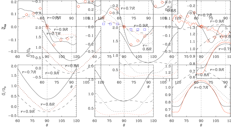
Figure 6: Latitudinal profiles of $\tilde{Q}_{\theta\phi}$ and $\tilde{\Omega}$ for Runs A4, A5, and A6 (from left to right) at three different depths (solid 0.7$R$, dotted 0.8$R$, dashed 0.9$R$). The red dotted lines show data from corresponding Runs B1, B2, and B3 from $r=0.8R$. The solid red lines in the right panels show data from Run D2 at $r=0.8R$. The open red diamonds in the top panels denote Cartesian Runs cA1–cA4, cD1–cD4, and cE1–cE4, from left to right. The blue squares in the top-middle panel show the values of $Q_{yz}$ computed from Fourier-filtered velocity fields from Runs cD1–cD4. Note that only a part of the full latitudinal range is shown.

We find that the horizontal stress, $\tilde{Q}_{\theta\phi}$, is almost always positive (negative) in the northern (southern) hemisphere for ${\rm Co}<1$, i.e. antisymmetric about the equator, see Fig. 5. For intermediate rotation (Runs A4 and A5) the stress is observed to change sign at high latitudes. In Fig. 6 we plot the latitudinal profiles of the horizontal stress and the mean angular velocity at different depths for the Runs A4–A6. It can be seen that near the bottom of the convection zone, the profile of the stress becomes more and more concentrated about the equator as the Coriolis number increases. An especially abrupt change can be observed for Run A5 (${\rm Co}\approx 2$). A similar peak also persists in Runs A6, B3, C1, and D2 with the largest Coriolis numbers. Note, however, that the sign of the latitudinal differential rotation changes as ${\rm Co}$ increases to six for Run A6. The results of Robinson & Chan (RC01 (2001)) also show a peak of $Q_{\theta\phi}$, occurring at a latitude range $10\degr\ldots 15\degr$, depending on depth.

Using Eqs. (29)–(30), we can calculate the stress $Q_{\theta\phi}=\sum_{l,l^{\prime},m}Q_{\theta\phi}^{ll^{\prime}m}$ by azimuthal averaging, with

$$Q_{\theta\phi}^{ll^{\prime}m}=\frac{1}{2}v_{\rm P}^{lm}w_{\rm T}^{l^{\prime}m}\left(\frac{1}{r^{2}}\frac{\partial P_{l}^{m}}{\partial\theta}\frac{\partial P_{l^{\prime}}^{m}}{\partial\theta}-\frac{m^{2}}{\varpi^{2}}P_{l}^{m}P_{l^{\prime}}^{m}\right),$$

where $P_{l}^{m}(\theta)$ are the associated Legendre polynomials and $\varpi=r\sin\theta$. Note that $l$ and $l^{\prime}$ denote the degrees of the poloidal and the toroidal flow, respectively. It is easy to see that the contribution to the azimuthally averaged $Q_{\theta\phi}$ is always zero from cross-correlation between two poloidal velocity fields. Finite contributions to $Q_{\theta\phi}$ instead come from correlations between poloidal flow and toroidal flow having the same azimuthal degree $m$. We have used small-scale velocity fluctuations (i.e., $m\neq 0$ modes) to calculate the Reynolds stresses in the numerical simulations according to Eq. (34). The finite correlation of the rotation and the meridional flow are not included in this discussion since both are characterised by $m=0$ and thus do not correspond to our definition of velocity fluctuations.

Recently, Bessolaz & Brun (BB11 (2011)) have used wavelets and autocorrelation techniques to unravel the structure of giant cells in their 3-dimensional hydrodynamic convection simulations. It is an involved exercise to calculate the net stress by estimating the power in each triplet $(l,l^{\prime},m)$ by wavelet analysis. It is, however, possible to look for certain combinations of Legendre polynomials that can contribute to the peaks of $Q_{\theta\phi}$ near the equator as obtained from numerical simulations in spherical geometry. A visual inspection of the radial flows in Fig. 3 for Run B2 shows four prominent banana cells within the domain which extends from $0$ to $\pi/4$ in the azimuthal direction, which means that the angular dependence is most likely $Y_{16}^{16}$. Hence we set $l=16,l^{\prime}=16,17$ for the calculation of the stresses and vary $m$ in search for a match between the peaks of $Q_{\theta\phi}$ from the runs A1–A6 and Eq. (3.1). We illustrate the angular part of $Q_{\theta\phi}^{ll^{\prime}m}$, for particular values of $l,l^{\prime}$ and $m$ in Fig. 7. We can see from here that peaks in $Q_{\theta\phi}^{16,17,15}$ (dashed line) appear at $\pm 6^{\circ}$ as well as at $\pm 20^{\circ}$ latitude, whereas peaks in $Q_{\theta\phi}^{16,17,16}$ appear at $\pm 10^{\circ}$ latitude, and the highest peaks in $Q_{\theta\phi}^{16,17,8}$ appear at $\pm 60^{\circ}$ latitude. Comparing Fig. 5 with Fig. 7, we see that at slow rotation (Runs A1 and A2), a major contribution to the stress may come from giant cells with an angular dependence $Y_{16}^{8}$. At higher $\rm Co$, the stress may have contributions from banana cells with angular dependence $Y_{16}^{16}$ (compare solid line in top right panel of Fig. 6 with solid line of Fig. 7). We shall return to the question regarding the contribution of banana cells in the context of Cartesian runs in Sect. 3.2.1. However there also exists symmetric contribution to $Q_{\theta\phi}$ from components like $Q_{\theta\phi}^{16,16,16}$, but we do not see any significant symmetric part in the horizontal stresses from the numerical simulations. On this basis, zonal flows of the form $w_{\rm T}^{ll}\hat{\bm{r}}\times\bm{\nabla}Y_{l}^{l}$ can be said to be negligible in spherical convection simulations. These zonal flows correspond to a row of horizontal vortices with their centres on the equator.

Finally, let us discuss the stress component $Q_{r\theta}$. It does not directly contribute to angular momentum transport, but it can be important in generating or modifying meridional circulation, and it has routinely been considered also in earlier studies (e.g., Pulkkinen et al. Pea93 (1993); Rieutord et al. RBMD94 (1994); Käpylä et al. KKT04 (2004)). Figure 8 shows the stress component $Q_{r\theta}$ from Set A. We find that for slow rotation (Run A1) the stress is quite weak and shows several sign changes as a function of latitude. It is not clear whether this pattern is real or an artefact of insufficient statistics. For intermediate rotation (Runs A2–A4), $Q_{r\theta}$ shows an antisymmetric profile with respect to the equator being positive in the northern hemisphere and negative in the south, in accordance with earlier Cartesian results (e.g. Käpylä et al. KKT04 (2004)). Although the theory for this stress component is not as well developed as that of the other two off-diagonal components, Rüdiger et al. (2005a ) state that $Q_{r\theta}$ should always be negative in the northern hemisphere, which is at odds with our results. However, in our rapid rotation models (Runs A5–A6) the sign is found to change.

3.2 Comparison with Cartesian simulations

Before describing the Reynolds stress obtained from our simulations in Cartesian coordinates, we note that the rms velocities in the Cartesian runs are in general almost twice as large as in the spherical ones with the same input parameters (compare, e.g., Run A0 in Table 1 and Run cA0 in Table 2). We argue in Sect. 3.3 that this is the result of adopting a radial dependence of gravity in the plane-parallel atmosphere.

Figure 7: Angular part of $Q_{\theta\phi}^{ll^{\prime}m}$ normalized by the maximum value for four different cases characterized by triplets $(l,l^{\prime},m)$ as indicated by the legend. The latitudes of the peaks for the triplets are indicated on the respective curves.

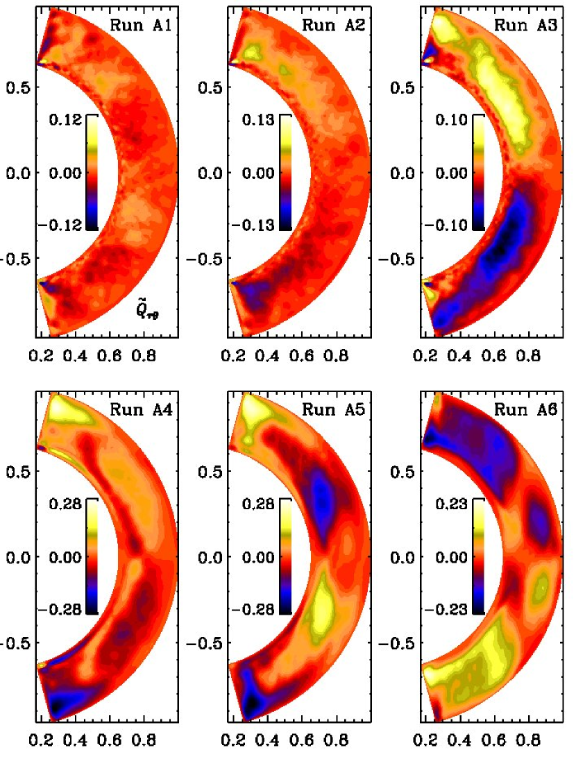
Figure 8: Meridional Reynolds stress, $\tilde{Q}_{r\theta}$, from Set A.

Table 2: Summary of the runs in Cartesian coordinates.

$$\begin{array}[]{p{0.05\linewidth}ccccccc}\hline\cr\vskip 3.0pt plus 1.0pt minus 1.0pt\cr Run&$Latitude$&{\rm Re}&{\rm Co}&{\rm Ma}&\tilde{E}_{\rm k}&E_{\rm mer}/E_{\rm k}&E_{\rm rot}/E_{\rm k}\\ \hline\cr cA0&-&63&0.00&0.038&1.7\cdot 10^{-4}&0.052&0.001\\ cF0&-&28&0.00&0.027&2.3\cdot 10^{-4}&0.021&0.001\\ cF1&-&11&0.00&0.022&2.5\cdot 10^{-4}&0.002&0.000\\ \hline\cr cA1&0^{\circ}&64&0.85&0.039&2.9\cdot 10^{-4}&0.001&0.288\\ cA2&7^{\circ}&65&0.84&0.039&2.0\cdot 10^{-4}&0.021&0.017\\ cA3&14^{\circ}&65&0.84&0.039&1.8\cdot 10^{-4}&0.014&0.007\\ cA4&21^{\circ}&65&0.85&0.039&1.8\cdot 10^{-4}&0.012&0.008\\ \hline\cr cB1&0^{\circ}&61&1.49&0.037&4.5\cdot 10^{-4}&0.000&0.623\\ cB2&7^{\circ}&70&1.30&0.042&2.4\cdot 10^{-4}&0.023&0.012\\ cB3&14^{\circ}&68&1.33&0.041&2.0\cdot 10^{-4}&0.012&0.007\\ cB4&21^{\circ}&68&1.34&0.041&1.9\cdot 10^{-4}&0.005&0.009\\ \hline\cr cC1&0^{\circ}&60&2.14&0.036&2.8\cdot 10^{-4}&0.000&0.347\\ cC2&7^{\circ}&76&1.68&0.046&2.5\cdot 10^{-4}&0.029&0.031\\ cC3&14^{\circ}&72&1.77&0.044&2.2\cdot 10^{-4}&0.013&0.011\\ cC4&21^{\circ}&72&1.78&0.043&2.1\cdot 10^{-4}&0.004&0.011\\ \hline\cr cD1&0^{\circ}&69&2.38&0.042&7.5\cdot 10^{-4}&0.000&0.584\\ cD2&7^{\circ}&78&2.09&0.047&2.5\cdot 10^{-4}&0.029&0.018\\ cD3&14^{\circ}&47&2.32&0.043&2.0\cdot 10^{-4}&0.009&0.013\\ cD4&21^{\circ}&70&2.36&0.042&2.1\cdot 10^{-4}&0.003&0.005\\ \hline\cr cE1&0^{\circ}&50&3.66&0.045&1.2\cdot 10^{-3}&0.000&0.685\\ cE2&7^{\circ}&36&4.00&0.041&1.6\cdot 10^{-4}&0.025&0.009\\ cE3&14^{\circ}&34&4.24&0.039&1.5\cdot 10^{-4}&0.005&0.005\\ cE4&21^{\circ}&31&4.67&0.035&1.3\cdot 10^{-4}&0.001&0.008\\ \hline\cr\end{array}$$

The radial profiles of the three off-diagonal components of the Reynolds stress in Cartesian coordinates agree with previous studies (Käpylä et al. KKT04 (2004); Hupfer et al. HKS05 (2005)) for the range of latitudes and Coriolis number explored here (compare Fig. 9 with bottom panel of Fig. 11 of Käpylä et al. KKT04 (2004) and Figs. 3 and 5 of Hupfer et al. HKS05 (2005)). For moderate rotation (Runs cA1–cA4), the vertical component $\tilde{Q}_{xz}$ (left panels of Fig. 9) is negative in the bottom part of the convection zone and almost zero at the top. The cases with ${\rm Co}\approx 2.3$ (Runs cD1–cD4) show negative values at the bottom and positive values at the top of the convection zone. For ${\rm Co}\approx 4.0$ (Runs cE1–cE4), the amplitude of the positive part of the stress near the surface increases and the negative part at the bottom decreases. We notice that the spatial distribution of $\tilde{Q}_{xz}$, as well as its variation with the Coriolis number, are in a fair agreement with the corresponding spherical runs in the same range of ${\rm Co}$ (Runs A3–A5). In the spherical Run A6 with the highest Coriolis number of roughly six, the stress is observed to become predominantly positive in the convection zone. This is not seen in the Cartesian counterparts that reach Coriolis numbers of roughly four (Runs cE1–cE4), in which the negative peak near the bottom still persists, although it has decreased in magnitude. The difference is possibly due to the lower Coriolis number in the Cartesian runs. It is noteworthy that also the symmetry of this stress component with respect to the equator is captured by the Cartesian simulations.

Radial profiles of the horizontal stress, $\tilde{Q}_{yz}$, from the Cartesian simulations are shown in the middle panels of Fig. 9, and latitudinal profiles in Fig. 6 with open squares and diamonds. Similarly as in the spherical runs, this component peaks both at top and bottom of the convective layer. However, some discrepancies are observed between the profiles in different geometries. For instance, in spherical Run A4 the stress is somewhat more widely distributed than in the corresponding Cartesian runs. In spherical Run A5 the radial profile of this component exhibits a bump at the bottom of the convection zone which is much larger than in the corresponding Cartesian cases. Note, however, that in Fig. 9, the uppermost peak moves inwards with increasing rotation between Sets cA and cD, and at the same time as the lowermost peak increases in amplitude. For the spherical Run A6 with the highest Coriolis number of roughly six, the stress changes sign in the region near the surface, which is not visible in the Cartesian simulations with Coriolis numbers of roughly four (Runs cE1–cE4).

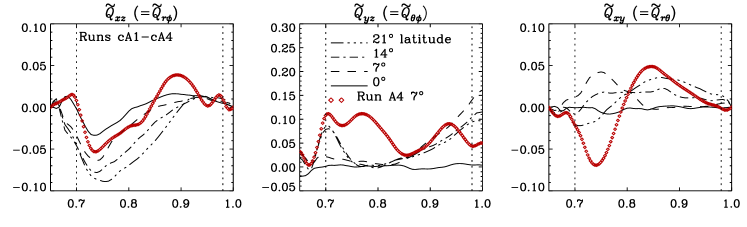
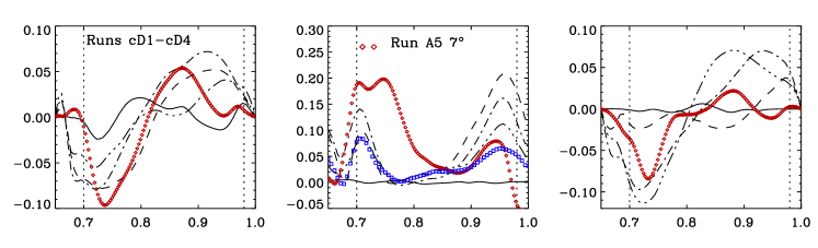
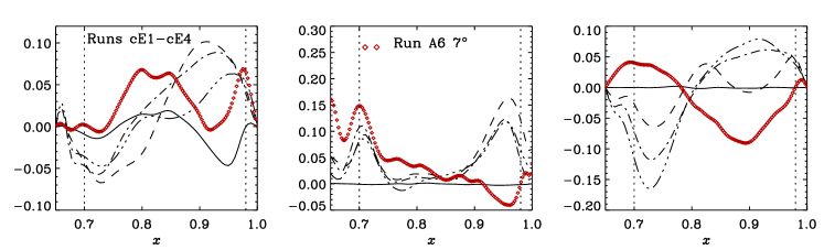
Figure 9: From left to right: radial profiles of $\tilde{Q}_{xz}$, $\tilde{Q}_{yz}$, and $\tilde{Q}_{xy}$ from Cartesian Runs cA1–cA4 (top panels), Runs cD1–cD4 (middle panels), and Runs cE1–cE4 (bottom panels). The red diamonds correspond to the radial profiles of the stresses in the spherical Runs A4–A6. The blue squares in the middle panel show Fourier-filtered data from Run cD2.

Finally, the meridional Reynolds stress, $\tilde{Q}_{xy}$, corresponding to $\tilde{Q}_{r\theta}$, is positive in the entire convection zone for moderate rotation (Runs cA1–cA4). For larger ${\rm Co}$, $\tilde{Q}_{xy}$ is negative in the lower part of the domain (see the right panels of Fig. 9). Similar behaviour occurs in the spherical case with intermediate rotation (Runs A3–A5). In the most rapidly rotating case (Run A6) another sign change occurs near the equator (see Fig. 8), which is not observed in Cartesian runs. This, however, could again be explained by the smaller ${\rm Co}$ in the Cartesian runs.

3.2.1 Filtering banana cells

The large amplitude of the horizontal Reynolds stress, peaking around $\pm 7\degr$ latitude, has been an intriguing issue for several years (e.g., Chan C01 (2001); Hupfer et al. HKS05 (2005, 2006)). One factor that might be contributing to the Reynolds stress are the large-scale banana cell-like flows that develop near the equator (e.g., Käpylä et al. KKT04 (2004); Chan C07 (2007)). Such flows vary in the azimuthal ($z$) direction and can lead to overestimation of the contribution of turbulence, especially if averaging is performed over the azimuthal ($z$) direction. We explore this possibility by filtering out the contribution coming from the large-scale structures observed in the $yz$-plane (the so-called banana cells observed in spherical simulations). The procedure used in this analysis is described below.

We perform a Fourier decomposition of the horizontal velocities and find out at which Fourier mode the contribution of the large scales peaks in the spectra. We find that the maximum is usually situated at wavenumber $q=2$. Next we remove this mode from the spectra and make an inverse Fourier transformation, thus obtaining the velocity field without the contribution from the large-scale motions. Finally, we compute $Q_{yz}$ from the filtered velocities.

Horizontal stress $Q_{yz}$ computed from filtered velocity fields for Runs cD1–cD4 for different latitudes at $r=0.9R$ are plotted with blue square symbols in Fig. 6. The radial variation of $Q_{yz}$ at $7\degr$ for Run cD2 is shown with blue square symbols in Fig. 9. It is clear from these figures that the $q=2$ mode is the dominant contribution to $Q_{yz}$ near the surface and it also affects significantly the secondary peak in deeper layers. Thus, a flatter profile in latitude with a reduced amplitude of the stress is obtained in comparison to the non-filtered values. The maximum, however, still resides around $\pm 7\degr$, which is at odds with theory (e.g. Rüdiger & Kitchatinov RK07 (2007)).

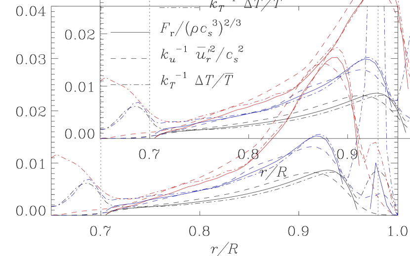
Figure 10: Normalized radial turbulent heat flux raised to the 2/3 power as a function of $r$ ($x$) (solid lines). The dashed and dot-dashed lines correspond to the squares of the radial velocity and temperature fluctuations scaled with the coefficients $k_{u}$ and $k_{T}$, respectively. The upper (red), middle (blue) and lower (black) curves correspond to Runs cA0, cF0 and A0, respectively.

3.3 Turbulent heat transport

In non-rotating convection the radial heat flux,

$$F_{r}=c_{\rm P}\overline{\rho}\overline{u_{r}^{\prime}T^{\prime}},$$ (35)

transports all of the energy through the convection zone. According to mixing length theory, velocity and temperature fluctuations are related via $\overline{u_{r}^{\prime 2}}\sim(\Delta T/\overline{T})g\ell$, where $\ell$ is the mixing length, $g\ell=c_{\rm s}^{2}$, and $\Delta T=\sqrt{\overline{T^{\prime 2}}}$. Thus, the three quantities are related via:

$$\frac{\Delta T}{\overline{T}}\sim\frac{\overline{u_{r}^{\prime 2}}}{c_{\rm s}^{2}}\sim\left(\frac{F_{r}}{\rho c_{\rm s}^{3}}\right)^{2/3}.$$ (36)

These quantities are shown in Fig. 10 for non-rotating simulations in Cartesian (Run cA0) and spherical (Run A0) geometries. Here we use the coefficients

$$k_{u}=\frac{\langle\overline{u_{r}^{\prime 2}}/c_{\rm s}^{2}\rangle_{\rm CZ}}{\langle F_{r}/\rho c_{\rm s}^{3}\rangle^{2/3}_{\rm CZ}}\leavevmode\nobreak\ ,\quad k_{T}=\frac{\langle\Delta T/\overline{T}\rangle_{\rm CZ}}{\langle F_{r}/\rho c_{\rm s}^{3}\rangle^{2/3}_{\rm CZ}}\leavevmode\nobreak\ ,$$ (37)

where $\langle.\rangle_{\rm CZ}$ denotes an average over the convection zone. For both geometries we obtain $k_{u}\approx 0.4$ and $k_{T}\approx 1.3$, values that are in good agreement with previous results (Brandenburg et al. BCNS05 (2005)). Note, however, that the magnitude of the flux in Cartesian coordinates is around four times larger than that in the spherical one, implying a difference of $4^{1/3}\approx 1.6$ in the radial velocities according to Eq. (37). This is roughly the same factor seen in the rms velocities (compare Runs A0 and cA0). This difference arises from the fact that we are considering a depth dependent gravity also in the Cartesian simulations. In spherical geometry, the luminosity is constant and the flux decreases outwards proportional to $r^{-2}$, whereas in Cartesian geometry the flux is constant. This means that for the same profile of thermal conductivity, a significantly larger portion of the energy is transported by convection in the Cartesian case. We verify this result with a separate Cartesian model in which the radiative flux is constant and, like in the other models, the gravity varies with depth. In this case the thermal conductivity varies with radius. The profiles of the quantities depicted in Fig. 10 obtained from this run (see blue lines and Run cF0 in Table 2) are in better agreement with the spherical case. Similar results have been obtained if both, radiative flux and gravity, are constant (Run cF1).

Figure 11: Turbulent heat conductivity $\chi_{\rm t}$ from Runs A0 (solid line) and B0 (dashed line). The inset shows the radial heat flux $F_{r}$ (solid line) and an analytical expression given in Eq. (40) (dashed line) normalized by the heat flux at $r_{1}$ from Run A0.

The radial turbulent heat transport may also be described in terms of a turbulent heat conductivity (e.g. Rüdiger R89 (1989))

$$F_{r}=c_{\rm P}\overline{\rho}\overline{u_{r}^{\prime}T^{\prime}}\equiv-\overline{\rho}\overline{T}\chi_{\rm t}\nabla_{r}\overline{s},$$ (38)

from which we can solve the turbulent heat conductivity as

$$\chi_{\rm t}=-\frac{c_{\rm P}\overline{u_{r}^{\prime}T^{\prime}}}{\overline{T}\nabla_{r}\overline{s}}.$$ (39)

The result, normalized by a reference value $\chi_{\rm t0}=u_{\rm rms}/(3k_{\rm f})$, for Runs A0 and B0 are shown in Fig. 11. Here averages over longitude and latitude are considered. We find that the value of $\chi_{\rm t}$ is almost ten times the reference value. The apparently large value is most likely due to the normalization factor which is based on a volume average of the rms velocity and a more or less arbitrary length scale $k_{\rm f}^{-1}$ (see also Käpylä et al. 2010b ). The sharp peaks and negative values of $\chi_{\rm t}$ towards the bottom and top of the convectively unstable region reflect the sign change of the entropy gradient which is not captured by Eq. (39).

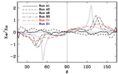
Figure 12: Off-diagonal component $\chi_{\theta r}$ of the turbulent heat conductivity according to Eq. (43) from Runs A1 (solid line), A3 (dashed), A6 (dot-dashed), B3 (triple-dot-dashed), C1 (red dashed), and D1 (blue dotted).

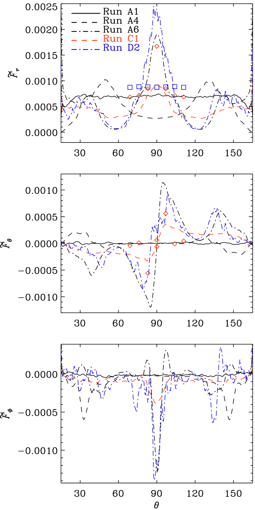
Figure 13: Turbulent heat fluxes $\tilde{F}_{r}$ (top panel), $\tilde{F}_{\theta}$ (middle), and $\tilde{F}_{\phi}$ (bottom) from the runs indicated in the legend in the top panel. The symbols included in the top and middle panels correspond to vertical and latitudinal fluxes from Runs cA1–cA4 (blue squares) and cE1–cE4 (red diamonds) scaled down by a factor of four (see the text for details). The data for Runs C1 and D2 are scaled up by a factor of four.

According to first-order smoothing (e.g. Rüdiger R89 (1989)), the radial flux can be written as

$$F_{r}^{\rm(FOSA)}=-\tau_{\rm c}\overline{u_{r}^{2}}\leavevmode\nobreak\ \overline{\rho}\leavevmode\nobreak\ \overline{T}\nabla_{r}\overline{s},$$ (40)

where $\tau_{\rm c}$ is the correlation time of turbulence. We compare the actual radial heat flux with the rhs of Eq. (40) in the inset of Fig. 11, where $\tau_{\rm c}$ is used as a fit parameter. A reasonable fit within the convection zone is obtained if the Strouhal number

$${\rm St}=\tau_{\rm c}u_{\rm rms}k_{\rm f},$$ (41)

is around 1.6 which is consistent with previous results from convection (e.g. Käpylä et al. 2010b ). Note that the ratio $\chi_{\rm t}/\chi_{\rm t0}$ gives a measure of the Strouhal number because in the general case $\chi_{\rm t0}={\textstyle{1\over 3}}\tau_{\rm c}u_{\rm rms}^{2}={\rm St}u_{\rm rms}/(3k_{\rm f})$, whereas in the main panel of Fig. (11) we assume ${\rm St}=1$.

In rotating convection, Eq. (38) no longer holds and the heat flux becomes latitude-dependent. In mean-field theory this can be represented in terms of an anisotropic turbulent heat conductivity (Kitchatinov et al. KPR94 (1994))

$$\chi_{ij}=\chi_{\rm t}\delta_{ij}+\chi_{\Omega}\varepsilon_{ijk}\hat{\Omega}_{k}+\chi_{\Omega\Omega}\hat{\Omega}_{i}\hat{\Omega}_{j},$$ (42)

where $\delta_{ij}$ and $\varepsilon_{ijk}$ are the Kronecker and Levi–Civita tensors and $\hat{\Omega}_{i}$ is the unit vector along the $i$th component of $\bm{\Omega}$. This indicates that non-zero latitudinal and azimuthal heat fluxes are also present in rotating convection. However, in order to compute all relevant coefficients from Eq. (42), a procedure similar to the test scalar method (Brandenburg et al. BSV09 (2009)) would be required in spherical coordinates. In most of our runs, however, the radial gradient of entropy is greater than the latitudinal one. Thus we can approximate the latitudinal heat flux by

$$F_{\theta}=-\overline{\rho}\overline{T}\chi_{\theta r}\nabla_{r}\overline{s}-\overline{\rho}\overline{T}\chi_{\theta\theta}\nabla_{\theta}\overline{s}\approx-\overline{\rho}\overline{T}\chi_{\theta r}\nabla_{r}\overline{s},$$ (43)

from which the off-diagonal component $\chi_{\theta r}$ can be computed in analogy to Eq. (39). Note that the sign of $\chi_{\theta r}$ gives the direction of the latitudinal heat flux so that positive (negative) values indicate equatorward (poleward) in the northern (southern) hemisphere. According to Eqs. (42) and (43), $F_{\theta}\propto\sin\theta\cos\theta$, indicating a sign change at the equator.

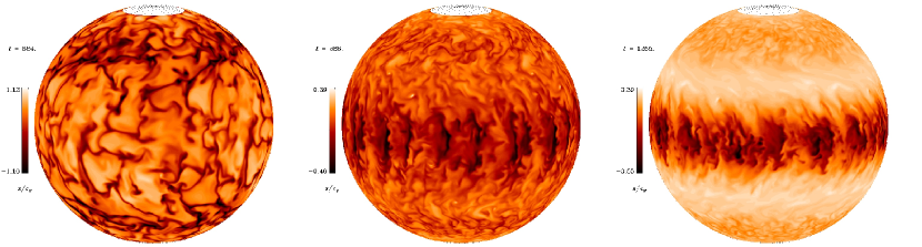
Figure 14: Specific entropy in the upper part of the convectively unstable layer in Runs B1 (left), D1 (middle), and D2 (right). The $\phi$-extent is duplicated fourfold for visualization purposes.

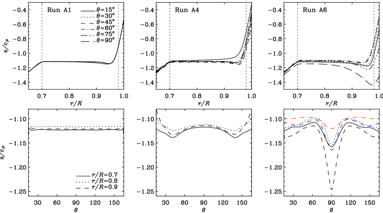
Figure 15: Top row: radial profiles of entropy from six colatitudes as indicated by the legend in the leftmost panel from Runs A1 (left column), A4 (middle column), and A6 (right column). Bottom row: latitudinal entropy profiles for the same runs as in the upper row at three radial positions indicated by the legend in the left panel. The red and blue dashed curves in the lower right panel show data at $r=0.9R$ from Runs C1 and D2, respectively.

Representative results from Runs A1, A3, A6, B3, C1, and D1 are shown in Fig. (12). For slow rotation (Run A1), $\chi_{\theta r}$ is small and shows no coherent latitude dependence. In the intermediate rotation regime (Run A3), $\chi_{\theta r}$ is positive (negative) in the northern (southern) hemisphere. In the most rapidly rotating case (Runs A6 and B3), the sign changes so that the heat flux is towards the poles. Qualitatively similar results are obtained from rapidly rotating Runs C1 and D1 with a lower Mach number. The smoother latitude profile of $\chi_{r\theta}$ in Run C1 reflects the smoother entropy profile (see Fig. 15). The qualitative behaviour as a function of rotation is similar to that found in local simulations (Käpylä et al. KKT04 (2004)). Comparing with Fig. 11 we find $\chi_{\theta r}/\chi_{\rm t}\equiv\chi_{\theta r}/\chi_{rr}\approx 0.1$, which is of the same order of magnitude as in local convection models Käpylä et al. (KKT04 (2004)) and forced turbulence Brandenburg et al. (BSV09 (2009)). We note that the latitudinal entropy gradient, which we neglected in Eq. (43), can become comparable with the radial one in the rapid rotation regime near the equator. Since $\nabla_{\theta}\overline{s}<0$ in the northern hemisphere (cf. Fig. 15), the latter term in Eq. (43) yields a positive contribution to the flux. Thus our values of $\chi_{\theta r}$ near the equator are likely to be underestimated in the rapid rotation regime. We postpone a more detailed study of the turbulent transport coefficients to a future publication and discuss the different components of the turbulent heat fluxes. We present the components of convective energy flux as

$$\tilde{F}_{i}=F_{i}/\overline{\rho}\,\overline{c_{\rm s}}^{3},$$ (44)

where longitudinal averages are used.

Figure 13 shows the normalized turbulent heat fluxes as functions of latitude from five runs with slow (Run A1), intermediate (Run A4), and rapid (Runs A6, C1, and D2) rotation. We find that $\tilde{F}_{r}$ shows little latitudinal variation except near the latitudinal boundaries for slow and moderate rotation (Runs A1–A3). For intermediate rotation $F_{r}$ peaks at mid latitudes (Runs A4–A5) whereas in the most rapidly rotating cases (Runs A6, C1, and D2) the maxima occur near the equator and at the latitudinal boundaries. This behaviour follows the trend seen in the entropy profile (Fig 15): the radial gradient of entropy shows only a minor variation as a function of latitude in the most slowly rotating runs (A1–A3). In Runs A4 and A5 the gradient is the steepest at mid latitudes and at the equator in Run A6. We find that the entropy gradient can become positive at certain latitudes, e.g. close to the pole for Run A4 and around latitudes $\pm 30\degr$ in Run A6.

The horizontal fluxes, $F_{\theta}$ and $F_{\phi}$ are negligibly small in comparison to the radial flux $F_{r}$ in the slow rotation regime (Run A1). The latitudinal flux is consistent with zero for all depths in Run A1 (see Fig. 13). For intermediate rotation (Runs A2–A4) the latitudinal flux is mostly equatorward. For the most rapidly rotating cases the sign changes so that in Runs A6, C1, and D2, $\tilde{F}_{y}$ is mostly poleward in the convection zone. The magnitude of the latitudinal flux also increases so that the maximum values, which are located near the surface, can become comparable with the radial flux. The azimuthal flux is also small and always negative, i.e., in the retrograde or westward direction, in accordance with the results of Rüdiger et al. (2005a ) and Brandenburg et al. (BSV09 (2009)).

In some of the panels in Fig. 13 we also present results from Cartesian simulations (see the red and blue symbols) from the same depth. As discussed above, the fluxes are larger in this geometry, due to which we have scaled the fluxes down by a factor of four in this figure. We find that the latitude profiles of the radial and latitudinal heat fluxes in the Cartesian simulations are in rather good agreement with the spherical results. This is more clear in the rapidly rotating cases cE1–cE4 in comparison to Run A6 (see the right panels of Fig. 13), where the large peak of $F_{r}$ at the equator, and the sharp peak of $F_{\theta}$ at low latitudes are reproduced.

We find that the latitudinal entropy profiles show a local maximum (slow and intermediate rotation) or a minimum (rapid rotation) at the equator, see Fig. 14 and the bottom panels of Fig. 15. The entropy profiles in the most rapidly rotating simulations (Run A6 and B3) are similar to that obtained by Miesch et al. (Mea00 (2000)) but differs from the more monotonic profiles of e.g. Brun et al. (BT02 (2002)) and the lower Mach number case Run C1.

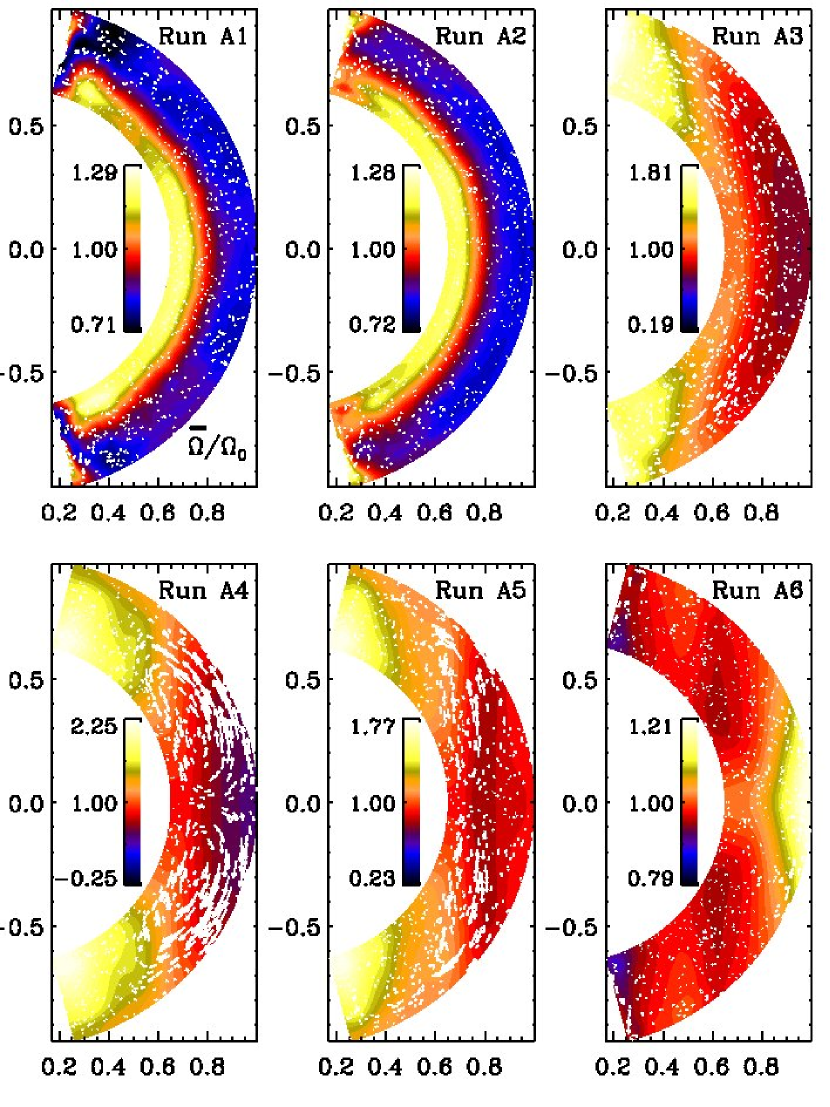
Figure 16: Azimuthally averaged flows from the runs in Set A. The contours show $\overline{\Omega}=\overline{u}_{\phi}/(r\sin\theta)+\Omega_{0}$ and the white arrows denote the meridional circulation.

3.4 Large-scale flows

The rotation profiles from the runs in Set A are shown in Fig. 16. For slow rotation (Runs A1–A2), a clear large-scale radial shear, almost independent of latitude, develops. This is an old result going back to Kippenhahn (Kip63 (1963)) that is expected for turbulence whose vertical motions dominate over horizontal ones (Rüdiger R89 (1989)). Such a result has been obtained in many mean-field models (e.g. Brandenburg et al. BMRT90 (1990)) and simulations since then (Brun & Palacios BP09 (2009), who refer to such flows as shellular). However, the $\Omega$–profiles in these runs are clearly different at high latitudes, which is probably an artefact due to the latitudinal boundaries. As the Coriolis number is increased, the radial shear remains negative, equatorial deceleration grows, and the isocontours of $\Omega$ tend to align more with the rotation vector (Runs A3–A4) – in accordance with the Taylor–Proudman theorem. Similar anti-solar rotation profiles have been reported also by Rieutord et al. (RBMD94 (1994)), Dobler et al. (DSB06 (2006)), Brown (B09 (2009)), and Chan (C10 (2010)). Such rotation profiles are usually the result of strong meridional circulation (Kitchatinov & Rüdiger KR04 (2004)) which is consistent with the present results. Run A5 represents a transitory case where bands of faster and slower rotation appear, whereas in Run A6 a solar-like equatorial acceleration is seen. Similar transitory profiles have recently been reported by Chan (C10 (2010)). The rotation profile in Run A6 is dominated by the Taylor–Proudman balance and the latitudinal shear is concentrated in a latitude strip of $\pm 30\degr$ about the equator. Similar $\Omega$–profiles have been obtained earlier from more specifically solar-like simulations (e.g., Brun & Toomre BT02 (2002); Brun et al. BMT04 (2004); Brown et al. BBBMT08 (2008); Ghizaru et al. GCS10 (2010)).

In the slow rotation regime (Runs A1–A2) the kinetic energy of meridional circulation and differential rotation are comparable and comprise a few per cent of the total kinetic energy (columns 9 and 10 in Table 1). Increasing the Coriolis number further, increases the fraction of kinetic energy in the differential rotation whereas that of the meridional circulation remains at first constant (Runs A3–A4), and finally drops close to zero (Runs A5–A6). In the three most rapidly rotating cases the differential rotation comprises more than 80 per cent of the total kinetic energy. We also find that the meridional circulation shows a coherent pattern only for intermediate rotation rates (Runs A3–A5) where a single counter-clockwise cell per hemisphere appears. In Run A6 the meridional flow is concentrated in a number of small cells in accordance with earlier results (e.g., Miesch et al. Mea00 (2000); Brun & Toomre BT02 (2002)). We note that the rotation profiles in Runs B3, C1, and D2 are similar to that in Run A6.

The surface differential rotation of stars can be observationally studied using photometric time series (e.g. Hall Hall91 (1991)) or with Doppler imaging methods (for a review, see Collier-Cameron CC07 (2007)). The amount of surface differential rotation has been determined for some rapidly rotating pre- or main-sequence stars with varying spectral type (F, G, K, and M), systematically showing solar-type differential rotation pattern with a faster equator and slower poles. The strength of the differential rotation shows a clear trend as function of the effective temperature, the shear being larger for hotter stars (see Fig. 1 of Collier-Cameron CC07 (2007)). Analysis of photometric time series, interpreting the period variations seen in the light curve analysis being due to differential rotation (e.g. Hall Hall91 (1991)), have established a relation $\Delta\Omega/\Omega_{0}\approx\Omega^{-n}$, with the values of $n\approx$ 0.8–0.9. The observational results are in rough agreement with theoretical predictions (e.g. Kitchatinov & Rüdiger KR99 (1999)), the theory predicting slightly weaker differential rotation in the rapid rotators than the actually observed values.

Figure 17: Differential rotation parameter $k_{\Omega}$ according to Eq. (45) from Sets A (stars), B (diamonds), Run C1 (cross), and Runs D1 and D2 (triangles). The dotted horizontal line indicates the zero level.

We parameterise the differential rotation in our simulations with the quantity

$$k_{\Omega}\equiv\frac{\Omega_{\rm eq}-\Omega_{\rm pole}}{\Omega_{\rm eq}}=\frac{\Delta\Omega}{\Omega_{\rm eq}},$$ (45)

where $\Omega_{\rm eq}=\overline{\Omega}(r_{4},\theta=90\degr)$ and $\Omega_{\rm pole}=\overline{\Omega}(r_{4},\theta=\theta_{0})$. The results for the runs with ${\rm Co}\neq 0$ listed in Table 1 are shown in Fig. 17. We find that the anti-solar differential rotation peaks at ${\rm Co}\approx 1$ and that $k_{\Omega}$ turns positive for roughly ${\rm Co}\approx 3$. The values in the rapid rotation ($k_{\Omega}\approx 0.2$) end are comparable with the Sun (see also Chan C10 (2010)). It is not clear, however, how realistic it is to compare the current simulations with observations, i.e. even to argue that slowly rotating stars have anti-solar differential rotation. It is clear that in the Sun the Coriolis number, and the radial length scale of convection, vary much more than in the current models so that it is not possible to reproduce equatorial acceleration and surface shear layer self-consistently in a single simulation. The situation may be different in slow rotators but observing their differential rotation is much more difficult. However, investigating the scaling of $k_{\Omega}$ in the rapid rotation regime is likely worth pursuing (see also Brown et al. BBBMT08 (2008)).

4 Conclusions

The present results have demonstrated that the basic properties of Reynolds stress and turbulent heat flux found in Cartesian simulations are reproduced by simulations in spherical shells and wedges. This includes the signs of the off-diagonal components of $Q_{ij}$. In particular, the vertical stress, $Q_{r\phi}$, is negative in both hemispheres when ${\rm Co}$ is small, but becomes positive near the top (and possibly also deeper down) when ${\rm Co}$ is large. This trend is well reproduced by the Cartesian simulations where $Q_{xz}$ is also negative for small ${\rm Co}$, but becomes positive near the top when ${\rm Co}$ is large. These results coincide with earlier findings of Käpylä et al. (KKT04 (2004)), Chan (C01 (2001)), and Robinson & Chan (RC01 (2001)).

The horizontal stress $Q_{\theta\phi}$, with the counterpart $Q_{yz}$ in the Cartesian model, is found to be positive in the northern hemisphere and have local maxima near the top and bottom of the domain. In spherical runs $Q_{\theta\phi}$ is found to change sign near the poles for intermediate rotation. For rapid rotation, $Q_{yz}$ reaches a maximum near the top (or surface) around $\pm 7^{\circ}$ latitude – in agreement with earlier results (e.g., Chan C01 (2001); Hupfer et al. HKS05 (2005)). We show that large-scale velocities due to the banana cells near the equator are the main contribution to $Q_{yz}$ in Cartesian calculations. The spherical simulations reproduce such a sharp peak in the regime ${\rm Co}\gtrsim 1$, the peak being limited to a radially narrow region near the bottom of the domain. We find that the results for the Reynolds stress are weakly dependent on the Reynolds and Mach numbers.

Furthermore, we find that $Q_{r\theta}$ is positive in the northern hemisphere, although for large values of ${\rm Co}$ the sign changes at the bottom of the convection zone. For the largest value of ${\rm Co}$, $Q_{r\theta}$ is negative throughout the entire convection zone. A similar trend is seen in the Cartesian simulations, where $Q_{xy}$ is mostly positive but becomes negative near the bottom of the convection zone when rotation becomes strong enough, in accordance with Käpylä et al. (KKT04 (2004))

The radial heat flux shows a strong dependence on latitude only when rotation is fairly rapid, i.e. ${\rm Co}\gtrsim 1$. This is associated with regions of the convection zone where the radial entropy gradient is decreased or even becomes positive. A partial explanation is that our setup (with a polytropic index of $n=1$) is such that roughly 80 per cent of the energy is transported by radiative diffusion (cf. Brandenburg et al. BCNS05 (2005)), making convection more easily suppressed than in a system where convection transports a larger fraction. The latitudinal heat flux is equatorward for slow rotation and changes sign around ${\rm Co}\approx 1$. A poleward heat flux is often used in breaking the Taylor–Proudman balance (e.g. Brandenburg et al. BMT92 (1992)). Longitudinal heat flux is mostly in the retrograde direction irrespective of the rotation rate.

The turbulent heat conductivity $\chi_{\rm t}$ is comparable to the first-order smoothing estimate with Strouhal number of the order of unity. The off-diagonal component $\chi_{\theta r}$ is typically an order of magnitude smaller than the diagonal component $\chi_{\rm t}$ in the rapid rotation regime. Similar results have been obtained previously from local convection simulations (e.g. Pulkkinen et al. Pea93 (1993)) and forced turbulence (Brandenburg et al. BSV09 (2009)). In mean-field models where anisotropic heat transport is invoked to break the Taylor–Proudman balance, the anisotropic part is typically of the same order of magnitude as the isotropic contribution (e.g. Brandenburg et al. BMT92 (1992)). It is conceivable that the anisotropic contribution increases when the fraction of convective energy flux is increased. However, such a study is not within the scope of the present paper.

As discussed in Sect. 3.1, the components of the Reynolds stress have contributions from diffusive and non-diffusive components. In future work we hope to be able to separate these two contributions, but in order to compare with earlier work, we have restricted ourselves to studying the components of the Reynolds stress directly. By making reasonable assumptions about the turbulent viscosity, it is indeed possible to obtain the relevant components of the $\Lambda$-effect, as was done by Pulkkinen et al. (Pea93 (1993)). This is also true of global models, which also yield directly the global flow properties that can then be compared with corresponding mean field models, as was first done by Rieutord et al. (RBMD94 (1994)). In a steady state, the Reynolds stress from the mean flow must then balance both the viscous stress and the Reynolds stress from the fluctuations, as was demonstrated also by Miesch et al. (MBDRT08 (2008)). Such results are, however, dependent on the particular properties of the model.

In the present paper we find that in the slow and intermediate rotation regimes the differential rotation is anti-solar: the equator is rotating slower than the high latitudes. Such rotation profiles also coincide with the occurrence of coherent meridional circulation that is concentrated in a single counter-clockwise cell. In the rapid rotation regime, solar-like equatorial acceleration is obtained, but the differential rotation is confined to latitudes $\pm 30\degr$ and the isocontours are aligned with the rotation vector.

To reproduce the solar rotation profile at least two major obstacles remain. Firstly, the Taylor–Proudman balance must be broken. A possibility is to use subgrid-scale models where the present results for anisotropic heat transport can work as a guide. Secondly, the Coriolis number should decrease near the surface so that the transport of angular momentum is inward near the surface, leading to a surface shear layer as in the Sun. Here we can again introduce a subgrid-scale Reynolds stress guided by the present results. Studying such models, however, is postponed to future papers.

Appendix A Dependence on domain size

Table 3: Summary of the runs with varying $\Delta\theta$ and $\Delta\phi$.

$$\begin{array}[]{p{0.05\linewidth}ccccccccccccc}\hline\cr\vskip 3.0pt plus 1.0pt minus 1.0pt\cr Run&$grid$&\theta_{1}&\Delta\theta&\Delta\phi&{\rm Ra}&{\rm Ma}&{\rm Re}&{\rm Co}&E_{\rm ther}&E_{\rm kin}&E_{\rm mer}/E_{\rm kin}&E_{\rm rot}/E_{\rm kin}&\Delta\Omega/\Omega_{\rm eq}\\ \hline\cr A5&128\times 256\times 128&15\degr&150\degr&90\degr&3.1\cdot 10^{6}&0.022&36&2.56&0.111&9.9\cdot 10^{-4}&0.002&0.949&-0.37\\ \hline\cr E1&128\times 256\times 32&15\degr&150\degr&22.5\degr&3.1\cdot 10^{6}&0.019&31&2.91&0.113&7.0\cdot 10^{-4}&0.009&0.963&-0.43\\ E2&128\times 256\times 64&15\degr&150\degr&45\degr&3.1\cdot 10^{6}&0.020&33&2.77&0.112&7.7\cdot 10^{-4}&0.008&0.946&-0.35\\ E3&128\times 256\times 256&15\degr&150\degr&180\degr&3.1\cdot 10^{6}&0.022&37&2.47&0.113&1.1\cdot 10^{-3}&0.002&0.941&-0.41\\ E4&128\times 256\times 384&15\degr&150\degr&270\degr&3.1\cdot 10^{6}&0.023&39&2.36&0.111&8.3\cdot 10^{-4}&0.002&0.902&-0.29\\ E5&128\times 256\times 512&15\degr&150\degr&360\degr&3.1\cdot 10^{6}&0.025&41&2.23&0.112&4.0\cdot 10^{-4}&0.001&0.659&-0.05\\ \hline\cr F1&128\times 96\times 128&60\degr&60\degr&90\degr&3.1\cdot 10^{6}&0.033&31&2.92&0.115&1.3\cdot 10^{-4}&0.001&0.644&+0.12\\ F2&128\times 160\times 128&45\degr&90\degr&90\degr&3.1\cdot 10^{6}&0.020&32&2.82&0.114&4.7\cdot 10^{-4}&0.004&0.899&-0.13\\ F3&128\times 192\times 128&30\degr&120\degr&90\degr&3.1\cdot 10^{6}&0.021&34&2.68&0.113&4.3\cdot 10^{-4}&0.004&0.885&-0.08\\ F4&128\times 288\times 128&5\degr&170\degr&90\degr&3.1\cdot 10^{6}&0.020&34&2.71&0.113&3.7\cdot 10^{-4}&0.006&0.882&-0.07\\ \hline\cr\end{array}$$

Above we have shown that we can recover many earlier results obtained in full spherical shells with wedges that span 150°in latitude and 90° in longitude. This gives at least a fourfold advantage in terms of computation time in comparison to a full shell. However, it is important to study the range within which we can still recover the same results as with larger wedges. In order to study this we perform two additional sets of runs that are listed in Table 3. In Set E we vary the longitudinal extent from $22.5\degr$ to full $360\degr$, with $\Delta\theta=150\degr$ in all models. In Set F we keep the longitudinal extent fixed at $\Delta\phi=90\degr$ and vary the latitudinal extent between $60\degr$ and $170\degr$. As our base model we take Run A5 with fairly rapid rotation and complicated large-scale flows in the saturated state.

Figure 18 shows the latitudinal profiles of the off-diagonal components of the Reynolds stress from the middle of the convectively unstable layer and the rotation profiles as functions of radius from three latitudes from Set E and Run A5. The Reynolds stresses are very similar in the latitude range $\pm 45\degr$ in runs with $\Delta\phi=90\degr$ or larger. Somewhat larger differences are seen near the latitudinal boundaries. Runs E1 and E2 with the smallest longitude extents show the same qualitative behaviour for stress components $Q_{r\theta}$ and $Q_{\theta\phi}$ but not for $Q_{r\phi}$. The rotation profiles for Runs A5, E3, and E4 with $\Delta\phi=90\degr-270\degr$ are very similar. The most obvious deviations from the trend occur again for Runs E1 and E2 where the radial gradient of $\overline{\Omega}$ is negative at the equator as opposed to the other runs where a positive gradient is found for $r/R>0.8$. Surprisingly, Run E5 with a full $360\degr$ longitude extent also deviates from the trend seen in the intermediate $\phi$-extents: the qualitative trend of $\overline{\Omega}$ is similar but the magnitude of the differential rotation is reduced. This is due to a non-axisymmetric $m=2$ mode which is excited in this simulation. Large-scale hydrodynamical non-axisymmetries have been reported from rapidly rotating convection (e.g. Brown et al. BBBMT08 (2008)). However, it is not clear whether the non-axisymmetry in our Run E5 is due to the same mechanism because of the slower rotation.

Comparing simulations with different latitudinal extents (Fig. 19), we find that domains confined between $\pm 45\degr$ latitude still reproduce the essential features of the solutions. This is particularly clear for the Reynolds stresses which are very similar in the latitude range $\pm 45\degr$ from the equator, with only Run F1 showing qualitatively different results in this range. There are also some differences at high latitudes between Runs A5 and F4. The rotation profiles are also very similar in the range $\pm 30\degr$ with the exception of Run F1. Run A5 also shows a deviating profile at high latitudes.

These results suggest that a $90\degr$ longitude and $150\degr$ latitude extent is sufficient to capture the main features of the solutions at larger domains. The cost of this is that some features which are not of primary interest in the present study, such as the large-scale non-axisymmetric modes, are omitted.

Figure 18: Off-diagonal Reynolds stresses from the middle of the convection zone (upper row), and $\overline{\Omega}$ as a function of radius at $\theta=90\degr$ (lower row, left panel), $\theta=60\degr$ (middle panel), and $\theta=30\degr$ (right panel) for Runs E1–E5 and A5. Linestyles as indicated in the legend in the lower middle panel.

Figure 19: Same as Fig. 18 but for Runs F1–F4 and A5. The left panel on the lower row shows $\overline{\Omega}$ from $\theta=45\degr$. Linestyles as indicated in the legend in the lower left panel