Extension of the Morris-Shore transformation to multilevel ladders

Abstract

We describe situations in which chains of $N$ degenerate quantum energy levels, coupled by time-dependent external fields, can be replaced by independent sets of chains, of length $N$, $N-1$, $\ldots,2$, and sets of uncoupled single states. The transformation is a generalization of the two-level Morris-Shore transformation [J.R. Morris and B.W. Shore, Phys. Rev. A 27, 906 (1983)]. We illustrate the procedure with examples of three-level chains.

I Introduction

The two-level atom has become over the years the basic building block with which one describes resonant and near-resonant radiative excitation of atoms and molecules – or any system that has discrete quantum states All75 ; Sho90 . When the radiation emanates from a laser, and therefore retains temporal coherence, the relevant dynamics is governed by the time-dependent Schrödinger equation. Within the usual rotating-wave approximation (RWA) Sho90 , the needed mathematics is that of two coupled linear ordinary differential equations for two complex-valued time-dependent probability amplitudes. The relative simplicity of these two equations has enabled researchers to find a variety of analytic solutions, descriptive both of steady radiation intensity and pulsed excitation by a variety of analytic forms for the pulses. In essence, one is able to map the physics of the two-level atom, under suitable conditions, onto the wealth of special functions studied by 19th century mathematicians.

This basic two-state atom has an interesting extension, from a nondegenerate two-level system (one with just two quantum states – ground and excited), to one with a degenerate ground level and a degenerate excited level. This situation occurs quite commonly for isolated atoms and molecules; these can be taken to be in states of well defined angular momentum $J$, for which rotational symmetry produces a degeneracy of $2J+1$ magnetic sublevels. In RWA the degeneracies can also occur for more general multistate quantum systems, as we shall note.

For laser-induced transitions between states of angular momentum, one must consider the several magnetic sublevels, labeled by $M$, that may occur as possible initial states. Each of them has a possible laser-driven excitation route into excited magnetic sublevels. If the angular momenta of the ground level and the excited level are, respectively, $J$ and $J^{\prime}$ (with $J=J^{\prime}$ or $J^{\prime}\pm 1$ for electric-dipole transitions), and if all excited magnetic sublevels are linked with some ground level, then in general one must consider $2J+1+2J^{\prime}+1$ probability amplitudes, coupled to one another by radiative interactions.

For general polarization of the laser field selection rules restrict the change in magnetic quantum number to quantum states whose magnetic quantum numbers $M$ and $M^{\prime}$ differ by $\Delta M=-1$, 0 or +1. For an arbitrary choice of quantization axis, and elliptically polarized light, the excitation can take place via all of these linkages. However, when the polarization is more specialized, to linear or circular, then it is possible to choose a quantization axis such that these coupled equations become a set of $2J+1$ pairs of independent two-state equations. The choice of quantization axis, together with the properties of the rotation matrix of angular momentum states, makes this possible. For such situations the mathematics is much simpler: one need only find a set of independent solutions to the nondegenerate two-state systems.

In 1983 Morris and Shore showed Morris83 that this coordinate transformation was a special case of a more general transformation that could produce, for any two degenerate sets of quantum states, an equivalent description involving only independent uncoupled pairs of equations. Specifically, the Morris-Shore (MS) transformation reduces the coherent quantum dynamics of a coupled degenerate two-level system to a set of independent nondegenerate two-state systems and a number of uncoupled (dark) states. It prescribes a simple recipe, which only requires to find the eigenvalues and the eigenstates of a hermitean matrix, which is a product of interaction matrices. The eigenstates are the MS states (i.e. the states representing the independent two-state systems and the dark states), and the eigenvalues are the MS interactions in the independent MS two-state systems. The MS transformation requires that all initial interactions be constant, or share the same time dependence, and that all interactions are resonant, or equally detuned from the upper states, so that each pair of interactions are on two-photon resonance with the corresponding states; the latter condition implies that the lower set of states is degenerate in RWA sense, and so is the upper set of states.

The MS transformation has been used extensively in various excitation scenarios to handle seemingly complicated linkages. For instance, it has been used to derive exact analytic solutions that extend known two-state solutions to degenerate two-state systems MS-analytic . It has been used to design schemes for complete population transfer between degenerate states MS-CPT and for creation of coherent superpositions of states MS-sup . The MS transformation has been also a crucial analytic method in creating recipes for efficient discrete quantum state tomography MS-tomo .

There are many situations in which one is interested in transitions that link not just two states but a chain-like sequence of multilevel excitations. Typically these form an $N$-level ladder linkage pattern, involving with each link a separate laser field. When such a system has degeneracy only from angular momentum, and when the pulses all share a common time-dependent envelope (though not the same carrier frequencies), and when the polarizations are all linear or circular, then it is possible to choose the (arbitrary) quantization axis such that the entire excitation scheme can be reduced to $2J+1$ sets of $N$ coupled equations, where $J$ is the angular momentum of the initially populated level.

It is natural to ask whether the MS transformation of two levels has a generalization to $N$-level ladders. We here answer this question affirmatively, with the proviso of certain conditions, and describe the procedure for finding the transformation. Such a transformation allows one to use the well-known analytic solutions of the $N$-state ladder Bia77 ; Ebe77a ; Sho81b as an extension of the utilization of analytic two-state solutions.

This paper is organized as follows. In Sec. II we review the two-level MS transformation and set the stage for its extension. In Sec. III we describe a resonantly coupled multilevel ladder, which is reducible to the two-level case. Section IV presents in detail the most general, non-resonant extension of the MS transformation to three levels, and Sec. V extends these results to $N$ levels. Finally, Sec. LABEL:Sec-conclusions presents a summary of the results.

II The two-level Morris-Shore transformation

The original MS transformation adopts a state ordering wherein the $N_{a}$ sublevels of the $a$ level are placed first, followed by the $N_{b}$ sublevels of the $b$ level. This allows us to view the RWA Hamiltonian as a block matrix,

$$\mathsf{H}(t)=\left[\begin{array}[]{ll}\mathsf{O}&\mathsf{V}(t)\\ \mathsf{V}(t)^{\dagger}&\mathsf{D}\end{array}\right].$$ (1)

Here $\mathsf{O}$ is the $N_{a}$-dimensional square zero matrix, in which the zero off-diagonal elements reflect the absence of single-photon couplings between the $a$ states, while the zero diagonal elements show that the $a$ states have the same energy, taken as the zero of the energy scale. The matrix $\mathsf{D}$ is a $N_{b}$-dimensional square diagonal matrix, which can be represented as a constant multiple of the $N_{b}$-dimensional unit matrix $\mathsf{1}_{N_{b}}$, $\mathsf{D}=\Delta\mathsf{1}_{N_{b}}$. The absence of off-diagonal elements in $\mathsf{D}$ reflects the absence of direct couplings between the $b$ states, while the common diagonal elements $\Delta$ stand for the common detunings of all the $b$ states: by definition, $\Delta$ is the difference between the Bohr transition frequency and the laser carrier frequency. The $N_{a}\times N_{b}$ matrix $\mathsf{V}(t)$ comprises the interactions of the $a$ subevels with the $b$ sublevels; these may depend on time, but the time dependence must be the same for every element. As evident from Eq. (1), it is assumed that there are no relaxation processes during the interaction.

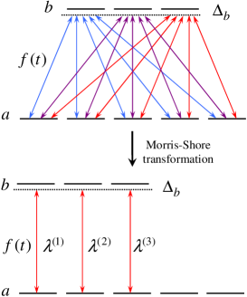
Figure 1: (Color online) The essence of the Morris-Shore transformation: a multistate system consisting of two coupled sets of degenerate levels is decomposed into a set of uncoupled nondegenerate two-state systems and a set of uncoupled (dark) states.

Although we shall discuss this Hamiltonian within the framework of angular momentum degeneracy, the results are applicable much more generally, to linkage patterns between nondegenerate states, as will occur when there are several different laser frequencies, each resonant (or near resonant) with a particular transition. When such situations are eligible for description by a multilevel RWA Sho90 , and when the carrier frequencies are such that at most two nonzero detunings occur in the RWA Hamiltonian, then the MS transformation can be used. Specifically, Morris and Shore have shown Morris83 that any RWA-degenerate two-level system, in which all couplings share the same time dependence, can be reduced with a constant unitary transformation to an equivalent system comprising only independent two-state systems and uncoupled (dark) states, as shown in Fig. 1. This time independent transformation is given by

$$\left|\psi_{i}\right\rangle=\sum_{k}S_{ki}^{\ast}\left|\varphi_{k}\right\rangle\quad\Longleftrightarrow\quad\left|\varphi_{k}\right\rangle=\sum_{i}S_{ki}\left|\psi_{i}\right\rangle.$$ (2)

The constant transformation matrix $\mathsf{S}$ can be represented in the block-matrix form

$$\mathsf{S}=\left[\begin{array}[]{cc}\mathsf{S}_{a}&\mathsf{O}\\ \mathsf{O}&\mathsf{S}_{b}\end{array}\right],$$ (3)

where $\mathsf{S}_{a}$ is a unitary $N_{a}$-dimensional square matrix and $\mathsf{S}_{b}$ is a unitary $N_{b}$-dimensional square matrix, $\mathsf{S}_{a}\mathsf{S}_{a}^{\dagger}=\mathsf{S}_{a}^{\dagger}\mathsf{S}_{a}=\mathsf{1}_{N_{a}}$ and $\mathsf{S}_{b}\mathsf{S}_{b}^{\dagger}=\mathsf{S}_{b}^{\dagger}\mathsf{S}_{b}=\mathsf{1}_{N_{b}}$. The constant matrices $\mathsf{S}_{a}$ and $\mathsf{S}_{b}$ mix only sublevels of a given level: $\mathsf{S}_{a}$ mixes the $a$ sublevels and $\mathsf{S}_{b}$ mixes the $b$ sublevels. The transformed MS Hamiltonian has the form (to simplify notation we here omit explicit display of time dependence)

$$\mathsf{H}^{MS}=\mathsf{S}\mathsf{H}\mathsf{S}^{\dagger}=\left[\begin{array}[]{cc}\mathsf{O}&\mathsf{M}\\ \mathsf{M}^{\dagger}&\mathsf{D}\end{array}\right],$$ (4)

where

$$\mathsf{M}=\mathsf{S}_{a}\mathsf{VS}_{b}^{\dagger}.$$ (5)

The $N_{a}\times N_{b}$ matrix $\mathsf{M}$ may have null rows (if $N_{a}>N_{b}$) or null columns (if $N_{a}<N_{b}$), which correspond to dark states; let us assume that $N_{a}>N_{b}$. The decomposition of $\mathsf{H}$ into a set of independent two-state systems requires that, after removing the null rows or columns, $\mathsf{M}$ reduces (possibly after an appropriate relabeling) to a diagonal matrix; let us denote its diagonal elements by $\lambda^{(n)}$ ($n=1,2,\ldots,N_{b}$). It follows from Eq. (5) that

$$\mathsf{M}\mathsf{M}^{\dagger} = \mathsf{S}_{a}\mathsf{V}\mathsf{V}^{\dagger}\mathsf{S}_{a}^{\dagger},$$ (6a)

$$\mathsf{M}^{\dagger}\mathsf{M} = \mathsf{S}_{b}\mathsf{V}^{\dagger}\mathsf{VS}_{b}^{\dagger}.$$ (6b)

Hence $$\mathsf{S}_{a} \mathsf{S}_{b} \mathsf{V}\mathsf{V}^{\dagger} \mathsf{V}^{\dagger}\mathsf{V} \mathsf{V} f(t) \mathsf{S}_{a} \mathsf{S}_{b} f^{2}(t)$$ and are defined by the condition that they diagonalize and , respectively. Because, by assumption, all elements of have the same time dependence , this dependence is factored out and therefore and are constant; the eigenvalues, however, are proportional to and hence they depend on time.

It is straightforward to show that the $N_{b}$ eigenvalues of $\mathsf{V}^{\dagger}\mathsf{V}$ are all non-negative; according to Eq. (6) they are $\left[\lambda^{(n)}\right]^{2}$. The matrix $\mathsf{V}\mathsf{V}^{\dagger}$ has the same eigenvalues and additional $N_{a}-N_{b}$ zero eigenvalues. The independent two-state systems $\varphi_{a}^{(n)}\leftrightarrow\varphi_{b}^{(n)}$ ($n=1,2,\ldots,N_{b}$), each composed of an $a$ state $\varphi_{a}^{(n)}$ and a $b$ state $\varphi_{b}^{(n)}$, are driven by the (time-varying) RWA Hamiltonians

$$\mathsf{H}^{(n)}=\left[\begin{array}[]{cc}0&\lambda^{(n)}\\ \lambda^{(n)}&\Delta\end{array}\right]\quad(n=1,2,\ldots,N_{b}).$$ (7)

Each of these two-state Hamiltonians has the same detuning $\Delta$; they differ in the Rabi frequency $2\lambda^{(n)}$.

III A multilevel Morris-Shore transformation: the quasi-two-level case

The two-level MS transformation is readily extended to multiple degenerate levels $a-b-c-d-\cdots$ when two conditions are fulfilled: (i) all couplings share the same time dependence (in particular, all couplings may be constant), and (ii) the two-photon resonances $a-c-\cdots$ and $b-d-\cdots$ are fulfilled (in particular, all fields may be on resonance with the respective transition frequency). This can be achieved by formally combining the RWA-degenerate sets $a,c,\ldots$ into one larger set of RWA-degenerate states, and the sets $b,d,\ldots$ into another larger set of RWA-degenerate states. Then one can carry out the MS factorization on the new degenerate two-level system, as displayed in Fig. 2. Then the MS states in the lower set will be superpositions of $a,c,\ldots$ states, whereas the MS states in the upper set will be superpositions of $b,d,\ldots$ states.

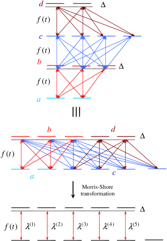
Figure 2: (Color online) The reducible multilevel Morris-Shore transformation in a multistate system consisting of $N$ coupled sets of degenerate levels when the two-photon resonances $a-c-\cdots$ and $b-d-\cdots$ are fulfilled (top). All interactions have the same time dependence $f(t)$. We first formally combine the RWA-degenerate sets $a,c,\ldots$ into one larger (“lower”) set of RWA-degenerate states, and the sets $b,d,\ldots$ into another larger (“upper”) set of RWA-degenerate states (middle). Then the new degenerate two-level system is decomposed into a set of independent nondegenerate two-state systems and a set of uncoupled (dark) states (bottom).

When the above conditions (i) or (ii) are not met, then we cannot reduce the multilevel case to a two-level one. Nevertheless, it may still be possible to replace the complicated linkages by simple sets of independent ladders. The next section presents a truly multilevel extension of the MS transformation that produces this reduction.

IV The three-level Morris-Shore transformation

IV.1 The RWA Hamiltonian

We consider excitation by a set of coherent laser pulses of a multilevel system for which the generalized RWA is applicable. The excitation dynamics is governed by the time-dependent Schrödinger equation for the coupled probability amplitudes $C_{n}(t)$. In matrix form it reads

$$i\frac{d}{dt}\mathbf{C}(t)=\mathsf{H}(t)\mathbf{C}(t).$$ (8)

The elements of the RWA Hamiltonian matrix $\mathsf{H}(t)$ (in units of $\hbar$) are detunings (on the diagonal) and time-dependent Rabi frequencies times $1/2$. For simplicity we shall, in the following, omit explicit time arguments.

Let us specialize this equation to a three-level system, wherein there are $N_{k}$ degenerate sublevels of level $k$, where $k$ runs over indices $a$, $b$ and $c$. For definiteness we assume that these degenerate levels form a ladder, i.e. $E_{a}<E_{b}<E_{c}$. Figure 3 shows a possible linkage pattern amongst the quantum states: those of level $a$ link only to those of level $b$, as do those of level $c$; we assume there are no direct linkages between the $a$ states and the $c$ states. These assumptions allow us to present the RWA Hamiltonian in the block-matrix form

$$\mathsf{H}=\left[\begin{array}[]{ccc}\mathsf{O}&\mathsf{V}_{1}&\mathsf{O}\\ \mathsf{V}_{1}^{{\dagger}}&\mathsf{D}_{b}&\mathsf{V}_{2}\\ \mathsf{O}&\mathsf{V}_{2}^{{\dagger}}&\mathsf{D}_{c}\end{array}\right].$$ (9)

Here the matrix $\mathsf{O}$ in the upper left corner is a $N_{a}$-dimensional square null matrix, where the null off-diagonal elements reflect the absence of radiative couplings amongst the $a$ sublevels, while the null diagonal elements originate with our (conventional) choice of RWA phases. The null matrices in the upper right and lower left corners indicate the absence of direct linkages between the $a$ states and the $c$ states. The square matrices $\mathsf{D}_{b}$ and $\mathsf{D}_{c}$ are scalar multiples of unit matrices of dimensions $N_{b}$ and $N_{c}$, respectively, $\mathsf{D}_{b}=\Delta_{b}\mathsf{1}_{N_{b}}$ and $\mathsf{D}_{c}=\Delta_{c}\mathsf{1}_{N_{c}}$. The scalars $\Delta_{b}$ and $\Delta_{c}$ are, respectively, the usual one- and two-photon detunings associated with the RWA. Although not shown explicitly, the interactions $\mathsf{V}_{1}$ and $\mathsf{V}_{2}$ may depend upon time. However, the elements of each matrix must share a common time dependence, say $f_{1}(t)$ for $\mathsf{V}_{1}$ and $f_{2}(t)$ for $\mathsf{V}_{2}$.

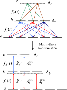
Figure 3: (Color online) The Morris-Shore transformation for three degenerate levels: the MS decomposition produces sets of independent nondegenerate three-state and two-state systems and a set of uncoupled (dark) states, provided the commutation condition (15) is fulfilled.

IV.2 The MS transformation

We wish to transform the original Hamiltonian (9) to a form in which the radiative couplings occur only in single unlinked chains, of length 2 or 3. That is, we seek a transformed MS basis, linked to the original basis by the transformation (2), and a corresponding transformed MS Hamiltonian, which must appear in the block form

$$\mathsf{H}^{MS}=\mathsf{SHS}^{{\dagger}}=\left[\begin{array}[]{ccc}\mathsf{O}&\mathsf{M}_{1}&\mathsf{O}\\ \mathsf{M}_{1}^{{\dagger}}&\mathsf{D}_{b}&\mathsf{M}_{2}\\ \mathsf{O}&\mathsf{M}_{2}^{{\dagger}}&\mathsf{D}_{c}\end{array}\right],$$ (10)

where $\mathsf{M}_{1}$ and $\mathsf{M}_{2}$ are diagonal matrices supplemented by null columns or rows.

The transformation must only combine sublevels within a given level. Therefore it must have the form

$$\mathsf{S}=\left[\begin{array}[]{ccc}\mathsf{S}_{a}&\mathsf{O}&\mathsf{O}\\ \mathsf{O}&\mathsf{S}_{b}&\mathsf{O}\\ \mathsf{O}&\mathsf{O}&\mathsf{S}_{c}\end{array}\right],$$ (11)

where $\mathsf{S}_{a}$, $\mathsf{S}_{b}$ and $\mathsf{S}_{c}$ are constant square unitary matrices of dimensions $N_{a}$, $N_{b}$, and $N_{c}$, respectively With this transformation the block elements of the transformed Hamiltonian (10) read

$$\mathsf{M}_{1} = \mathsf{S}_{a}\mathsf{V}_{1}\mathsf{S}_{b}^{{\dagger}},$$ (12a)

$$\mathsf{M}_{2} = \mathsf{S}_{b}\mathsf{V}_{2}\mathsf{S}_{c}^{{\dagger}}.$$ (12b)

The matrices $$\mathsf{M}_{1} \mathsf{M}_{2} \mathsf{H} \mathsf{M}_{1} \mathsf{M}_{2}$$ and may have null rows or columns; these correspond to dark states. The desired decomposition of into a set of independent two- or three-state systems requires that, after removing the null rows or columns, and reduce (possibly after an appropriate relabeling) to diagonal matrices. It follows from Eqs. (12) that the following matrices are diagonal:

$$\mathsf{S}_{a}\mathsf{V}_{1}\mathsf{V}_{1}^{{\dagger}}\mathsf{S}_{a}^{{\dagger}} = {\mathsf{M}_{1}\mathsf{M}_{1}}^{{\dagger}}=\text{diag},$$ (13a)

$$\mathsf{S}_{b}\mathsf{V}_{1}^{{\dagger}}\mathsf{V}_{1}\mathsf{S}_{b}^{{\dagger}} = \mathsf{M}_{1}^{{\dagger}}{\mathsf{M}_{1}}=\text{diag},$$ (13b)

$$\mathsf{S}_{b}\mathsf{V}_{2}\mathsf{V}_{2}^{{\dagger}}\mathsf{S}_{b}^{{\dagger}} = {\mathsf{M}_{2}\mathsf{M}_{2}}^{{\dagger}}=\text{diag},$$ (13c)

$$\mathsf{S}_{c}\mathsf{V}_{2}^{{\dagger}}\mathsf{V}_{2}\mathsf{S}_{c}^{{\dagger}} = \mathsf{M}_{2}^{{\dagger}}\mathsf{M}_{2}=\text{diag}\mathbf{.}$$ (13d)

Hence $$\mathsf{S}_{a} \mathsf{S}_{c} \mathsf{V}_{1}\mathsf{V}_{1}^{{\dagger}} \mathsf{V}_{2}^{{\dagger}}\mathsf{V}_{2} \mathsf{S}_{b} \mathsf{W}_{1} \mathsf{W}_{2}$$ and are defined by the condition that they diagonalize and , respectively. The matrix must, by definition, diagonalize both matrices and , where

$$\mathsf{W}_{1}=\mathsf{V}_{1}^{{\dagger}}\mathsf{V}_{1},\quad\mathsf{W}_{2}=\mathsf{V}_{2}\mathsf{V}_{2}^{{\dagger}}.$$ (14)

This can only occur if these two products commute,

$$\left[\mathsf{W}_{1},\mathsf{W}_{2}\right]=\mathsf{O}.$$ (15)

Hence ${\mathsf{W}_{1}}$ and $\mathsf{W}_{2}$ must have the same set of eigenvectors. This set, when normalized, forms the transformation matrix $\mathsf{S}_{b}$ for the $b$-state manifold. We shall assume hereafter that Eq. (15) is satisfied; we will discuss the implications of this assumption in Sec. IV.4.

It is easy to show that the eigenvalues of $\mathsf{V}_{1}\mathsf{V}_{1}^{{\dagger}}$ and $\mathsf{V}_{2}^{{\dagger}}\mathsf{V}_{2}$ are all non-negative, and hence they can be written as squares of real numbers, $\left[\lambda_{1}^{(n)}\right]^{2}$ and $\left[\lambda_{2}^{(n)}\right]^{2}$, respectively. The matrices $\mathsf{W}_{1}$ and $\mathsf{W}_{2}$ have the same eigenvalues, except for additional (or missing) zero eigenvalues.

In the MS basis, the description of the dynamics comprises sets of independent ladders, of length no greater than $N=3$. The three-state systems, expressing the linkages $a\leftrightarrow b\leftrightarrow c$, are governed by Hamiltonian matrices of the form

$$\mathsf{H}_{abc}^{(n)}=\left[\begin{array}[]{ccc}0&\lambda_{1}^{(n)}&0\\ \lambda_{1}^{(n)}&\Delta_{b}&\lambda_{2}^{(n)}\\ 0&\lambda_{2}^{(n)}&\Delta_{c}\end{array}\right].$$ (16)

Two-state systems $a\leftrightarrow b$, if present, are governed by the Hamiltonians

$$\mathsf{H}_{ab}^{(n)}=\left[\begin{array}[]{cc}0&\lambda_{1}^{(n)}\\ \lambda_{1}^{(n)}&\Delta_{b}\end{array}\right],$$ (17)

while two-state linkages $b\leftrightarrow c$ are governed by the Hamiltonians

$$\mathsf{H}_{bc}^{(n)}=\left[\begin{array}[]{cc}\Delta_{b}&\lambda_{2}^{(n)}\\ \lambda_{2}^{(n)}&\Delta_{c}\end{array}\right].$$ (18)

Finally, there may be single unlinked states, in any of the three levels; these can be regarded as being governed by one-dimensional matrices (scalars) $\mathsf{H}_{a}^{(n)}=0$ or $\mathsf{H}_{b}^{(n)}=\Delta_{b}$ or $\mathsf{H}_{c}^{(n)}=\Delta_{c}$.

In general, if the number of states in each initial manifold is different, we denote the minimum and maximum degeneracies by $N_{\min}\equiv\min\left\{N_{a},N_{b},N_{c}\right\}$, $N_{\max}\equiv\max\left\{N_{a},N_{b},N_{c}\right\}$, and the intermediate number by $N_{\text{mid}}$. We can then identify the following possibilities:

• if $N_{\min}=N_{b}$ then in the MS basis there will be $N_{b}$ three-state systems, $N_{a}-N_{b}$ dark states in the $a$ set of states, and $N_{c}-N_{b}$ dark states in the $c$ set;

• if $N_{\min}=N_{a}$ or $N_{c}$ then in the MS basis there will be $N_{\min}$ three-state systems, $N_{\text{mid}}-N_{\min}$ two-state systems composed of states of the sets with $N_{\text{mid}}$ and $N_{\max}$, and $N_{\max}-N_{\text{mid}}$ dark states composed of states of the set with $N_{\max}$.

Figure 3 shows an example in which the MS transformation reduces a general linkage pattern involving 10 states to a pair of dark states, a single two-state linkage, and a pair of three-state linkages. The time dependences $f_{1}(t)$ and $f_{2}(t)$ of the lower and upper transitions are arbitrary. In particular, the $f_{2}(t)$ interaction may precede the $f_{1}(t)$ interaction, as is the case of the STIRAP process STIRAP .

IV.3 Special case: single intermediate state

The commutation condition (15) is fulfilled automatically in the special case of a single, nondegenerate intermediate state, $N_{b}=1$, because then the matrices $\mathsf{W}_{1}^{{\dagger}}$ and $\mathsf{W}_{2}$ reduce to scalars. Then, regardless of the degeneracies $N_{a}$ and $N_{c}$ of states $a$ and $c$, the three-level MS transformation always produces a nondegenerate three-state system comprising a bright state from the $a$ level, a bright state from the $c$ level, and the intermediate state. In addition, there will be $N_{a}-1$ uncoupled states in the $a$ level and $N_{c}-1$ uncoupled states in the $c$ level. Hence for a single intermediate state the MS transformation is always possible. Figure 4 depicts an example of such a linkage pattern and the result of a MS transformation.

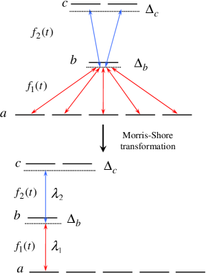
Figure 4: (Color online) The Morris-Shore transformation for a single nondegenerate intermediate state: the MS decomposition produces a nondegenerate three-state system and two sets of uncoupled (dark) states in the $a$ and $c$ sets of states.

IV.4 Consequences of the interaction commutation

We now turn to the implications of the commutation relation (15). This condition limits the generality of the MS transformation for three sets of degenerate states. We here pose the question: given the interaction $\mathsf{V}_{1}$, what is the most general form of the interaction $\mathsf{V}_{2}$, for which the three-level MS transformation applies?

IV.4.1 The Frobenius problem

The required commutation relation (15) is equivalent to solving a matrix equation of the form

$$\mathsf{AX}=\mathsf{XA}$$ (19)

for the matrix $\mathsf{X}$, given that $\mathsf{A}$ and $\mathsf{X}$ are both square Hermitian matrices of the same dimension $N_{b}$. This is known as the Frobenius problem Gantmacher . Because $\mathsf{A}$ and $\mathsf{X}$ commute, they have the same set of eigenvectors $\gamma_{n}$,

$$\mathsf{A}\gamma_{n} = \alpha_{n}\gamma_{n},$$ (20a)

$$\mathsf{X}\gamma_{n} = \xi_{n}\gamma_{n},$$ (20b)

and they are diagonalized by the same unitary matrix $$\mathsf{G}$$, composed of these eigenvectors,

$$\mathsf{G}{\mathsf{AG}}^{{\dagger}} = \mathsf{A}_{0}=\text{diag}\left\{\alpha_{1},\alpha_{2},\ldots,\alpha_{N_{b}}\right\},$$ (21a)

$$\mathsf{G}{\mathsf{XG}}^{{\dagger}} = \mathsf{X}_{0}=\text{diag}\left\{\xi_{1},\xi_{2},\ldots,\xi_{N_{b}}\right\}.$$ (21b)

Hence,

$$\mathsf{X}={\mathsf{G}}^{{\dagger}}{\mathsf{X}}_{0}{\mathsf{G}}.$$ (22)

We can view these results as follows. Given any Hermitian matrix $\mathsf{A}$, we can find the transformation matrix $\mathsf{G}$ which diagonalizes it. Then the most general form of the matrix $\mathsf{X}$ is the construction of Eq. (22), where the real diagonal matrix $\mathsf{X}_{0}$ is arbitrary. Therefore, if $\mathsf{A}$ and $\mathsf{X}$ are $N_{b}$-dimensional then the matrix $\mathsf{X}$ is parametrized by $N_{b}$ parameters: the diagonal elements of $\mathsf{X}_{0}$.

Alternatively, we can express the matrix $\mathsf{X}$ as a power series in $\mathsf{A}$. The Cayley-Hamilton theorem Gantmacher implies that only $N_{b}-1$ of these powers, e.g. $\mathsf{A}^{0}$, $\mathsf{A}^{1}$, $\ldots$, $\mathsf{A}^{N_{b}-1}$, are linearly independent. Then the expansion reads

$$\mathsf{X}=\sum_{n=0}^{N_{b}-1}x_{n}\mathsf{A}^{n},$$ (23)

where the $N_{b}$ coefficients $x_{n}$ are arbitrary. Because $\mathsf{X}$ is Hermitian, these numbers must be real.

Hence either of the two alternative solutions of the Frobenius problem (19) – either Eq. (22) or Eq. (23) – involve $N_{b}$ arbitrary real parameters.

IV.4.2 Implications for linkages

We now apply these results to the MS transformation. We know that any given interaction $\mathsf{V}_{1}$ determines the transformation matrix $\mathsf{S}_{b}$ through Eq. (13b). It follows that the interaction $\mathsf{V}_{2}$ must satisfy

$$\mathsf{W}_{2}={\mathsf{S}}_{b}^{{\dagger}}{\mathsf{W}}_{0}{\mathsf{S}}_{b},$$ (24)

with $\mathsf{W}_{2}=\mathsf{V}_{2}\mathsf{V}_{2}^{{\dagger}}$, where $\mathsf{W}_{0}$ is an arbitrary $N_{b}$-dimensional real diagonal matrix. Equation (23) implies that the most general representation of $\mathsf{W}_{2}$, for which the commutation relation (15) is satisfied and hence there exists MS transformation, has the form

$$\mathsf{W}_{2}=\sum_{n=0}^{N_{b}-1}w_{n}\mathsf{W}_{1}^{n}.$$ (25)

where the $N_{b}$ arbitrary real coefficients $w_{n}$ determine the degrees of freedom for $\mathsf{W}_{2}$.

IV.5 Example: $J=3/2\leftrightarrow J=1/2\leftrightarrow J=1/2$ ladder

IV.5.1 The system and the couplings

We here illustrate the rather formal results with a specific example. We consider a three-level ladder whose degeneracy stems from angular momentum. Specifically we consider the sequence $J=3/2\leftrightarrow J=1/2\leftrightarrow J=1/2$; hence the magnetic sublevels form a degenerate three-level system with $N_{a}=4$, $N_{b}=N_{c}=2$. Taking into account the Clebsch-Gordan coefficients Zar88 we find

$$\mathsf{V}_{1}(t) = \frac{f_{1}(t)}{\sqrt{6}}\left[\begin{array}[]{cc}r_{1}\sqrt{3}&0\\ -p_{1}\sqrt{2}&r_{1}\\ l_{1}&-p_{1}\sqrt{2}\\ 0&l_{1}\sqrt{3}\end{array}\right],$$ (26e)

$$\mathsf{V}_{2}(t) = \frac{f_{2}(t)}{\sqrt{3}}\left[\begin{array}[]{cc}-p_{2}&-r_{2}\sqrt{2}\\ l_{2}\sqrt{2}&p_{2}\end{array}\right],$$ (26h)

where $$f_{1}(t) f_{2}(t) r_{n},p_{n},l_{n} \sigma^{+} \pi \sigma^{-} n=1 n=2$$ anf define the (generally different) time envelopes of the pulsed interactions in the lower and upper transitions, respectively; are related to the amplitudes (with the respective phases) of the right-circular (), linear (), and left-circular () polarizations for the lower () or upper () transition.

IV.5.2 The MS states

The MS states in the $a$ manifold are defined as the eigenstates of the matrix $\mathsf{V}_{1}\mathsf{V}_{1}^{{\dagger}}$ [see Eq. (13a)],

$$\mathsf{V}_{1}\mathsf{V}_{1}^{{\dagger}}=\frac{f_{1}^{2}(t)}{6}\left[\begin{array}[]{cccc}3\left|r_{1}\right|^{2}&-\sqrt{6}p_{1}^{\ast}r_{1}&\sqrt{3}l_{1}^{\ast}r_{1}&0\\ -\sqrt{6}p_{1}r_{1}^{\ast}&2\left|p_{1}\right|^{2}+\left|r_{1}\right|^{2}&-\sqrt{2}\left(p_{1}l_{1}^{\ast}+p_{1}^{\ast}r_{1}\right)&\sqrt{3}l_{1}^{\ast}r_{1}\\ \sqrt{3}l_{1}r_{1}^{\ast}&-\sqrt{2}\left(p_{1}^{\ast}l_{1}+p_{1}r_{1}^{\ast}\right)&\left|l_{1}\right|^{2}+2\left|p_{1}\right|^{2}&-\sqrt{6}p_{1}l_{1}^{\ast}\\ 0&l_{1}r_{1}^{\ast}\sqrt{3}&-\sqrt{6}p_{1}^{\ast}l_{1}&3\left|l_{1}\right|^{2}\end{array}\right].$$ (26i)

Two of these eigenstates are dark, with zero eigenvalues, whereas the other two are bright, with eigenvalues $\left(\lambda_{1}^{(1)}\right)^{2}$ and $\left(\lambda_{1}^{(2)}\right)^{2}$; the explicit forms of these eigenstates are too cumbersome to be presented here.

The MS states in the $c$ manifold are defined as the eigenstates of the matrix $\mathsf{V}_{2}^{{\dagger}}\mathsf{V}_{2}$ [see Eq. (13d)],

$$\mathsf{V}_{2}^{{\dagger}}\mathsf{V}_{2}=\frac{f_{2}^{2}(t)}{3}\left[\begin{array}[]{cc}\left|p_{2}\right|^{2}-2r_{2}^{\ast}l_{2}&2\sqrt{2}i\text{Im}\left(p_{2}^{\ast}r_{2}\right)\\ 2\sqrt{2}i\text{Im}\left(p_{2}^{\ast}l_{2}\right)&\left|p_{2}\right|^{2}-2r_{2}l_{2}^{\ast}\end{array}\right].$$ (27)

They have eigenvalues $\left(\lambda_{2}^{(1)}\right)^{2}$ and $\left(\lambda_{2}^{(2)}\right)^{2}$. Explicitly, the $\lambda$’s are given by

$$\lambda_{1}^{(1,2)} = \frac{f_{1}(t)}{\sqrt{6}}\eta_{1}\left[2\left(1+\xi_{1}\right)\right.$$ (28a)

$$\mp\left.\sqrt{\varepsilon_{1}^{2}+2\xi_{1}\left(1+\sqrt{1-\varepsilon_{1}^{2}}\cos\alpha_{1}\right)}\right]^{1/2},$$

$$\lambda_{2}^{(1,2)} = \frac{f_{2}(t)}{\sqrt{3}}\eta_{2}\left[1+\xi_{2}\right.$$ (28b)

$$\mp\left.\sqrt{\varepsilon_{2}^{2}+2\xi_{2}\left(1+\sqrt{1-\varepsilon_{2}^{2}}\cos\alpha_{2}\right)}\right]^{1/2},$$

with $$(n=1,2)$$

$$\varepsilon_{n} = \frac{\left|l_{n}\right|^{2}-\left|r_{n}\right|^{2}}{\eta_{n}^{2}},$$ (29a)

$$\xi_{n} = \frac{\left|p_{n}\right|^{2}}{\eta_{n}^{2}},$$ (29b)

$$\eta_{n} = \sqrt{\left|l_{n}\right|^{2}+\left|r_{n}\right|^{2}},$$ (29c)

$$\alpha_{n} = \arg l_{n}^{\ast}r_{n}^{\ast}p_{n}^{2}.$$ (29d)

The MS states in the intermediate level $b$ are the common eigenstates of the matrices $\mathsf{W}_{1}=\mathsf{V}_{1}^{{\dagger}}\mathsf{V}_{1}$ and $\mathsf{W}_{2}=\mathsf{V}_{2}\mathsf{V}_{2}^{{\dagger}}$ [see Eqs. (13b) and (13c)], i.e.,

$$\mathsf{W}_{1}=\left[\begin{array}[]{cc}3\left|r_{1}\right|^{2}+2\left|p_{1}\right|^{2}+\left|l_{1}\right|^{2}&-\sqrt{2}\left(p_{1}^{\ast}r_{1}+p_{1}l_{1}^{\ast}\right)\\ -\sqrt{2}\left(p_{1}r_{1}^{\ast}+p_{1}^{\ast}l_{1}\right)&\left|r_{1}\right|^{2}+2\left|p_{1}\right|^{2}+3\left|l_{1}\right|^{2}\end{array}\right]\frac{f_{1}^{2}(t)}{6},$$ (30a)

$$\mathsf{W}_{2}=\left[\begin{array}[]{cc}\left|p_{2}\right|^{2}+2\left|r_{2}\right|^{2}&-\sqrt{2}\left(p_{2}l_{2}^{\ast}+p_{2}^{\ast}r_{2}\right)\\ -\sqrt{2}\left(p_{2}^{\ast}l_{2}+p_{2}r_{2}^{\ast}\right)&\left|p_{2}\right|^{2}+2\left|l_{2}\right|^{2}\end{array}\right]\frac{f_{2}^{2}(t)}{3}.$$ (30b)

If $$\mathsf{W}_{1} \mathsf{W}_{2} \mathsf{W}_{1} \mathsf{W}_{2} a-b b \mathsf{W}_{1} b b-c \mathsf{W}_{2} b \mathsf{W}_{1} \mathsf{W}_{2}$$ and do not commute, then the eigenstates of will differ from the eigenstates of and there will be no MS factorization. In other words, the two-state MS transformation, when applied to the lower transition , will produce MS states in the level (defined as the eigenstates of ), which will differ from the MS states in this same level produced by two-state MS transformation in the upper transition (defined as the eigenstates of ). Three-state MS transformation will only occur if these two sets of states are the same, a necessary and sufficient condition for which is the commutation of and .

IV.5.3 Commutation implications

The commutation relation (15) leads to the equations

$$\text{Im}\left[\left(l_{1}^{\ast}p_{1}+r_{1}p_{1}^{\ast}\right)\left(l_{2}p_{2}^{\ast}+p_{2}r_{2}^{\ast}\right)\right]=0,$$ (31a)

$$\left(l_{1}p_{1}^{\ast}+r_{1}^{\ast}p_{1}\right)(\left|r_{2}\right|^{2}-\left|l_{2}\right|^{2})=(\left|r_{1}\right|^{2}-\left|l_{1}\right|^{2})\left(l_{2}p_{2}^{\ast}+p_{2}r_{2}^{\ast}\right).$$ (31b)

Obviously, if all interactions are real, the first condition (31a) is satisfied automatically.

In the general case of complex interactions, one can solve this system of equations, for example, by considering two cases: when $\left|r_{1}\right|\neq\left|l_{1}\right|$ and $\left|r_{1}\right|=\left|l_{1}\right|$.

(i) For $\left|r_{1}\right|\neq\left|l_{1}\right|$, it is readily seen, by replacing the term $\left(l_{2}p_{2}^{\ast}+p_{2}r_{2}^{\ast}\right)$ from Eq. (31b) into Eq. (31a), that Eq. (31a) is satisfied identically; hence condition (15) requires only one condition to be fulfilled: Eq. (31b). The latter condition can be solved, for example, for $p_{2}$,

$$p_{2}=\frac{l_{2}\left(l_{1}^{\ast}p_{1}+r_{1}p_{1}^{\ast}\right)-r_{2}\left(l_{1}p_{1}^{\ast}+r_{1}^{\ast}p_{1}\right)}{\left|l_{1}\right|^{2}-\left|r_{1}\right|^{2}}.$$ (32)

Condition (32) restricts the amplitude of the linearly polarized field for the upper transition to be a function of the arbitrary amplitudes of the other fields. Because $p_{2}$ is complex-valued, condition (32) represents, in fact, two conditions: for the modulus and the phase of $p_{2}$.

(ii) For $\left|r_{1}\right|=\left|l_{1}\right|$, there are obviously two solutions. The first of these is $\left|r_{2}\right|=\left|l_{2}\right|$; then Eq. (31a) is also required because it is not satisfied automatically. The second solution is $l_{1}p_{1}^{\ast}+r_{1}^{\ast}p_{1}=0$; it fixes one of the phases of the lower-transition fields (e.g., $2\arg p_{1}=\pi-\arg l_{1}+\arg r_{1}$).

With either of these choices (i) or (ii) for the fields it is possible to reduce the original linkage pattern to a pair of three-state ladders and two uncoupled dark states, as shown in Fig. 5.

One special example for conditions (31) is when the left- and right-polarized fields for the lower transition have the same intensity and the same phase ($r_{1}=l_{1}$), and the linearly-polarized field is shifted in phase by $\pi/2$ with respect to them; then $l_{1}p_{1}^{\ast}+r_{1}^{\ast}p_{1}=0$. No restrictions are imposed on the couplings of the upper transition in this case.

In another simple example, the left- and right-polarized fields for the lower transition have the same intensity ($\left|r_{1}\right|=\left|l_{1}\right|$) and the same applies for the upper transition ($\left|r_{2}\right|=\left|l_{2}\right|$), and all interactions are real.

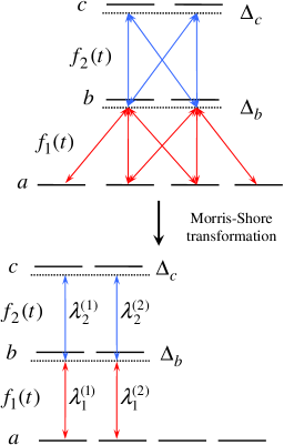
Figure 5: (Color online) The MS transformation for the three-level ladder $J=3/2\leftrightarrow J=1/2\leftrightarrow J=1/2$: the MS decomposition produces two independent nondegenerate three-state systems and two uncoupled (dark) states in the $J=3/2$ set.

IV.5.4 The MS picture

If the commutation relation (15) is satisfied then the Hamiltonian in the MS basis reads

$$\mathsf{H}^{MS}=\left[\begin{array}[]{cccccccc}0&0&0&0&0&0&0&0\\ 0&0&0&0&0&0&0&0\\ 0&0&0&0&\lambda_{1}^{(1)}&0&0&0\\ 0&0&0&0&0&\lambda_{1}^{(2)}&0&0\\ 0&0&\lambda_{1}^{(1)}&0&\Delta_{b}&0&\lambda_{2}^{(1)}&0\\ 0&0&0&\lambda_{1}^{(2)}&0&\Delta_{b}&0&\lambda_{2}^{(2)}\\ 0&0&0&0&\lambda_{2}^{(1)}&0&\Delta_{c}&0\\ 0&0&0&0&0&\lambda_{2}^{(2)}&0&\Delta_{c}\end{array}\right].$$ (33)

By rearranging the states, it is readily seen that there are two independent three-state systems driven by Hamiltonians of the form (16) ($n=1,2$), with MS couplings $\lambda_{1}^{(n)}$ and $\lambda_{2}^{(n)}$ given by Eqs. (28).

V Extension to $N$ levels

The results for the three-level MS transformation are readily extended to $N$ degenerate levels. For each transition $n$ ($n=1,2,\ldots,N-1$), described by an interaction matrix $\mathsf{V}_{n}$, time envelope $f_{n}(t)$ of all fields in this transition, and common detuning $\Delta_{n}$, we form the matrices $\mathsf{V}_{n}\mathsf{V}_{n}^{{\dagger}}$. The $N$-level MS transformation exists if

$$\left[\mathsf{V}_{n-1}^{{\dagger}}\mathsf{V}_{n-1},\mathsf{V}_{n}\mathsf{V}_{n}^{{\dagger}}\right]=\mathsf{O}\text{{\ (}}n=2,3,...,N-1\text{{).}}$$ (34)

The relations (34) imply that the interactions for any two adjacent transitions $n$ and $n+1$ must be such that, after the MS transformation, the resulting MS states of the common level of these two transitions are the same for the lower and upper transitions; mathematically this is ensured by the commutation of $\mathsf{W}_{n}$ and $\mathsf{W}_{n+1}$.

If conditions (34) are satisfied, the MS transformation will produce sets of independent nondegenerate $N$-state systems, $(N-1)$-state systems, and so on, and a number of uncoupled states, depending on the particular system.

VI Conclusions

In this paper, we have presented an extension of the MS transformation to three and more degenerate levels. For two degenerate sets of states the MS transformation always exists, as long as the couplings have the same time dependence and the same detunings. For three sets of states, the MS transformation may or may not exist, depending of the commutation of products of interaction matrices. When applicable, the MS transformation reduces the coupled multistate dynamics into a set of independent three-state systems, a set of independent two-state systems, and a number of uncoupled (dark) states. The number of states in each set depends on the degeneracy of the three initial sets of states. These results readily extend to $N$ degenerate levels, with similar commutation conditions on the interactions.

It is important that each set of states have the same RWA detuning, but this may differ from set to set. The couplings between the first and second set must have the same time dependence, and the same condition must apply between the second and third set; the two time dependences, however, may be different, as in STIRAP STIRAP . This condition extends to $N$ degenerate levels as well.

It is also important that any time dependence of the interactions is factored out of the commutation condition (34) and therefore, for instance, different time dependence of the transition $a-b$ with respect to the transition $b-c$ is possible. However, within each degenerate transition ($a-b$, $b-c$, $\ldots$) the time dependence must be the same; otherwise couplings appear between the MS states in each manifold, which create linkages between the independent MS subsystems and the MS decomposition does not occur.

If all detunings are zero (i.e. if all fields are on exact resonance with the respective transition frequency) and all fields share the same time dependence, the degenerate $N$-level system is reducible to a degenerate two-level system; then the original MS transformation decouples the interaction dynamics into a set of independent nondegenerate two-state systems and a set of dark states.

In the interesting special case of a three-level ladder with a single nondegenerate intermediate state, the MS transformation always exists, with no restrictions on the couplings (apart from the identical time dependence). The MS transformation produces a single linked chain, together with additional uncoupled states.

It is significant that the MS transformation, in producing a simplification of the original linkage pattern of interactions, introduces coherent superpositions of the original basis states. In this MS basis the dynamics appears very simple, and one can evaluate the conditions for producing complete population transfer, for example. Such transitions correspond, in the original basis, to transitions between coherent superposition states. When the initial state is nondegenerate then only the intermediate and final states of the transitions involve superposition states. Under such circumstances one can design pulse sequences that produce a specified superposition.

- (1) L. Allen and J. H. Eberly, Optical Resonance and Two-Level Atoms, (Wiley, New York, 1975).
- (2) B. W. Shore, The Theory of Coherent Atomic Excitation, (Wiley, N.Y., 1990).
- (3) J. R. Morris and B. W. Shore, Phys. Rev. A 27, 906 (1983).
- (4) N. V. Vitanov, Z. Kis, and B. W. Shore, Phys. Rev. A 68, 063414 (2003); E. S. Kyoseva and N. V. Vitanov, Phys. Rev. A 73, 023420 (2006).
- (5) Z. Kis, A. Karpati, B. W. Shore, and N. V. Vitanov, Phys. Rev. A 70, 053405 (2004).
- (6) Z. Kis, N. V. Vitanov, A. Karpati, C. Barthel, and K. Bergmann, Phys. Rev. A 72, 033403 (2005).
- (7) N. V. Vitanov, B. W. Shore, R. G. Unanyan, and K. Bergmann, Opt. Commun. 179, 73 (2000); N. V. Vitanov, J. Phys. B 33, 2333 (2000); P. A. Ivanov and N. V. Vitanov, Opt. Commun., accepted (2006).
- (8) Z. Bialynicka-Birula, I. Bialynicki-Birula, J. H. Eberly and B. W. Shore, Phys. Rev. A 16, 2048 (1977).
- (9) J. H. Eberly, B. W. Shore, Z. Bialynicka-Birula and I. Bialynicki-Birula, Phys. Rev. A 16, 2038 (1977).
- (10) B. W. Shore and M. A. Johnson, Phys. Rev. A 23, 1608 (1981).
- (11) K. Bergmann, H. Theuer and B.W. Shore, Rev. Mod. Phys. 70, 1003 (1998); N.V. Vitanov, M. Fleischhauer, B.W. Shore and K. Bergmann, Adv. At. Mol. Opt. Phys. 46, 55 (2001); N.V. Vitanov, T. Halfmann, B.W. Shore, and K. Bergmann, Ann. Rev. Phys. Chem. 52, 763 (2001).
- (12) F. R. Gantmacher, Matrix Theory (Springer, Berlin, 1986).
- (13) R. N. Zare, Angular Momentum: Understanding Spatial Aspects in Chemistry and Physics, (Wiley, N.Y., 1988).