The uses of the refined matrix model recursion

Abstract:

We study matrix models in the $\beta$-ensemble by building on the refined recursion relation proposed by Chekhov and Eynard. We present explicit results for the first $\beta$-deformed corrections in the one-cut and the two-cut cases, as well as two applications to supersymmetric gauge theories: the calculation of superpotentials in ${\cal N}=1$ gauge theories, and the calculation of vevs of surface operators in superconformal ${\cal N}=2$ theories and their Liouville duals. Finally, we study the $\beta$-deformation of the Chern–Simons matrix model. Our results indicate that this model does not provide an appropriate description of the $\Omega$-deformed topological string on the resolved conifold, and therefore that the $\beta$-deformation might provide a different generalization of topological string theory in toric Calabi–Yau backgrounds.

1 Introduction

Matrix models in the $1/N$ expansion have become a powerful tool in the study of supersymmetric gauge theories and string theories. For example, as shown by Dijkgraaf and Vafa in [19], the all-genus free energies of type B topological string theories on certain non-compact Calabi–Yau manifolds can be computed from the $1/N$ expansion of simple, polynomial matrix models, and this leads to exact results for the superpotentials of a large class of ${\cal N}=1$ supersymmetric theories [20]. Other applications include the matrix model formulation of Chern–Simons theories [45, 46] and the matrix model-inspired remodeling of the B-model [47, 8] for the mirrors of general toric geometries. As a consequence of these relationships, the recent progress in solving the $1/N$ expansion of matrix models [24, 27] has found many applications in string theory and gauge theory.

Most of these applications involve the standard Hermitian matrix model ensemble. There is a well-known one-parameter deformation of this ensemble, usually called the $\beta$-ensemble or the $\beta$-deformation, which involves an extra parameter $\beta$. The standard Hermitian ensemble is obtained when $\beta=1$, and the special values $\beta=2$ and $\beta=1/2$ correspond to ${\rm Sp}(N)$ real quaternionic and ${\rm SO}(N)$ real symmetric matrices, respectively. The $1/N$ expansion for the more general, $\beta$-deformed ensemble, has been worked out in an algebro-geometric language by Chekhov and Eynard [15, 14]. As in [24, 27], explicit expressions for the expansion of correlators and free energies are obtained through a “refined” recursion relation based on the spectral curve of the matrix model with $\beta=1$.

The general $\beta$ ensemble also has many applications. For example, the special values $\beta=2,1/2$ lead to the enumeration of non-orientable surfaces (see for example [11, 51]), and this can be used to construct non-critical unoriented strings in an appropriate double-scaling limit [11, 32] (see [18, 52] for a review of these ideas). These ensembles also appear naturally when one applies the techniques pioneered by Dijkgraaf and Vafa to supersymmetric gauge theories with ${\rm SO}(N)$ and ${\rm Sp}(N)$ gauge symmetry [43, 42, 3]. More recently, there has been renewed interest in the $\beta$-ensemble in the context of the so-called AGT correspondence between ${\cal N}=2$ gauge theories and Liouville theory [5]. In this correspondence, conformal blocks in Liouville theory are identified with $\Omega$-deformed partition functions [53] in ${\cal N}=2$ theories, and it has been argued in [21] that the general $\Omega$-deformation of ${\cal N}=2$ superconformal field theories can be implemented by a $\beta$-deformed matrix model with a Penner-type potential.

In this paper we analyze in detail the recursive proposal by Chekhov and Eynard and its concrete implementation in various examples. In section 2 we thoroughly study the algebro-geometric solution of the loop equations for the $\beta$-deformed eigenvalue model; in doing so, we first find a correction to the diagrammatic solution of [15], which was also very recently pointed out by Chekhov [14], and discuss various technical issues associated to the $\beta$-deformation with respect to the ordinary $\beta=1$ case. We moreover present explicit formulae for the very first corrections to correlators and free energies in the $\beta$-ensemble for a variety of situations and potentials; in the one-cut case and for polynomial potentials, some of these formulae were already derived in [30] and used there to analyze the universality properties of the asymptotic enumeration of graphs in non-orientable surfaces (see also the recent paper [7] for another derivation of explicit one-cut formulae). In section 3 we use these results to study applications to supersymmetric gauge theories. The first application is the computation of ${\cal N}=1$ superpotentials, where we recover and generalize previous results in [43, 42, 3, 35]. Our second application is to the AGT correspondence, where we consider surface operators [6, 41, 22] in a very simple example associated to a sphere with three punctures. In this case, we generalize the B-model computation in [41] and show that the $\beta$-deformed correlators obtained with the formalism of [15] lead to correlation functions in Liouville theory for general background charge.

One motivation for the present work was to find a matrix model formulation of topological string theory in an $\Omega$-background. This background provides a one-parameter deformation of topological string theory (at least on certain toric Calabi–Yau manifolds) which was originally obtained via a five-dimensional version of Nekrasov’s partition function [53]. The $\Omega$-deformed topological string was reformulated later on in terms of the refined topological vertex [36]. More recently, the holomorphic anomaly equation has been generalized to the $\Omega$-background for ${\cal N}=2$ gauge theories [44] and more generally for the A-model on local Calabi Yau manifolds [34], thus providing an important step towards a B-model version of this deformed theory.

It is natural to try to extend the remodeling of the B-model [8] to this deformation, and the refined recursion relation of Chekhov and Eynard is a natural candidate for this, as suggested by the arguments of [21] and by our computations in Section 3.2. In order to test this idea we analyze, in section 4, the $\beta$-deformed Chern–Simons (CS) matrix model of [45]. When $\beta=1$ this model is dual to type A topological string theory on the resolved conifold, and its $\beta$-deformation is a natural candidate for the $\Omega$-deformation of this theory. Our explicit computations, verified by perturbative calculations, show that the recursion of [15] works perfectly well for the CS matrix model, but unfortunately they do not seem compatible with the $\Omega$-deformation, at least when taken at face value (this was mentioned as well in [34]). An interesting feature we discover is a highly involved analytic dependence of $\beta$-deformed amplitudes on the closed string moduli with respect to their “refined” counterpart. This degree of sophistication only increases when moving to multi-cut models, where the exact formulae we find, e.g. for the cubic matrix model, display a more intricated analytic structure as compared to oriented, open amplitudes at higher genus [27, 8]. In particular, they cannot be immediately related to the same type of holomorphic quasi-modular forms of the ordinary topological string in a self-dual background [2], and it would be interesting to see what kind of generalization would be needed to encompass this more general case.

Our work indicates that the matrix model $\beta$-deformation can be defined and computed for the mirrors of other toric Calabi–Yau manifolds. An important example are the mirrors of $A_{p}$ fibrations over ${\mathbb{P}}^{1}$. These models can be described by Chern–Simons matrix models on lens spaces [1], and one can generalize the computation performed in section 4 to this more general setting. In fact, it is likely, in view of the progress in formulating the $\beta$-deformation in a geometric language [17], that the $\beta$-deformation provides a generalization of the B-model for the mirrors of toric Calabi–Yaus. According to our explicit results, it seems that this deformation will be in general different from the $\Omega$-deformation. If this is indeed the case it would be interesting to understand more aspects of this deformation. For example, one could use the Chekhov–Eynard recursion, together with the strategy of [26], to formulate a holomorphic anomaly equation for the $\beta$-deformed free energies. More generally, one should try to understand this deformation in the language of the A-model and in the gauge theory language.

2 Beta ensemble and topological recursion

In this section we review and analyze the formalism of Chekhov and Eynard [15], which proposes a topological recursion for the beta ensemble of random matrices. We will discuss the implementation of their formulae and present explicit expressions for various models.

2.1 General aspects

In terms of eigenvalues, the beta ensemble of random matrices is defined by the partition function

$$Z={1\over N!(2\pi)^{N}}\int\prod_{i=1}^{N}{\rm d}\lambda_{i}|\Delta(\lambda)|^{2\beta}{\rm e}^{-{\beta\over g_{s}}\sum_{i=1}^{N}V(\lambda_{i})}.$$ (2.1)

In what follows we will mainly follow the normalizations in [15]. The connected correlators are defined through

$$W(p_{1},\ldots,p_{h})=g_{s}^{2-h}\beta^{h-1}\left\langle{\rm Tr}\,{1\over p_{1}-M}\cdots{\rm Tr}\,{1\over p_{h}-M}\right\rangle^{(\mathrm{c})},\qquad h\geq 1.$$ (2.2)

The correlator $W(p)$ for $h=1$ is usually called the resolvent of the matrix model. Both the free energies and the connected correlators have an asymptotic expansion in $g_{s}$, in which the ’t Hooft parameters are kept fixed. In the case of the free energy $F=\log Z$, we have

$$F=\sum_{k,l\geq 0}g_{s}^{2k+l-2}\beta^{1-l/2-k}\gamma^{l}F_{k,l}.$$ (2.3)

where

$$\gamma={\sqrt{\beta}}-{\sqrt{\beta^{-1}}}.$$ (2.4)

For the first few terms we find, explicitly,

$$F =g_{s}^{-2}\beta F_{0,0}+g_{s}^{-1}(\beta-1)F_{0,1}+(\beta+\beta^{-1}-2)F_{0,2}+F_{1,0}$$ (2.5)

$$+g_{s}\left({(\beta-1)^{3}\over\beta^{2}}F_{0,3}+(1-\beta^{-1})F_{1,1}\right)$$

$$+g_{s}^{2}\left(\beta^{-1}F_{2,0}+{(\beta-1)^{2}\over\beta^{2}}F_{1,2}+{(\beta-1)^{4}\over\beta^{3}}F_{0,4}\right)+\cdots$$

The $g_{s}$ expansion of the connected correlators is written as

$$W(p_{1},\ldots,p_{h})=\sum_{g=0}^{\infty}\hbar^{2g}W_{g}(p_{1},\ldots,p_{h}),$$ (2.6)

where $g$ can be an integer or a half-integer, and $\hbar$ is defined as

$$\hbar={g_{s}\over{\sqrt{\beta}}}.$$ (2.7)

This expansion defines the “genus” $g$ correlators, which can be in turn expanded as

$$W_{g}(p_{1},\ldots,p_{h})=\sum_{k=0}^{[g]}\gamma^{2g-2k}W_{k,2g-2k}(p_{1},\cdots,p_{h}),$$ (2.8)

and leads to the following expansion for connected correlators,

$$\langle{\rm Tr}M^{n_{1}}\cdots{\rm Tr}M^{n_{h}}\rangle^{(c)}=\left({g_{s}\over\beta}\right)^{h}\sum_{g\geq 0}\sum_{k=0}^{[g]}\hbar^{2g-2}\gamma^{2g-2k}\langle{\rm Tr}M^{n_{1}}\cdots{\rm Tr}M^{n_{h}}\rangle^{(c)}_{k,l}.$$ (2.9)

The beta ensemble might be regarded as a natural deformation of the standard Hermitian ensemble, since when $\beta=1$ (2.1) becomes the standard partition function of the (gauged) Hermitian matrix model. In this case, in the expansion of the free energy and the correlators only the terms $F_{g,0}$ and $W_{g,0}$ contribute (with $g$ a non-negative integer). This leads to the standard expansion in powers of $g_{s}^{2}$ of the Hermitian matrix model. On the other hand, there are two special values of $\beta$ which have a matrix model realization: for $\beta=1/2$, (2.1) describes an ensemble of real symmetric matrices with orthogonal $SO(N)$ symmetry, while the case $\beta=2$ describes an ensemble of quaternionic real matrices with symplectic ${\rm Sp}(N)$ symmetry.

Example 2.1.

The Gaussian $\beta$ ensemble. In the Gaussian case

$$V(x)=x^{2}$$ (2.10)

the matrix integral (2.1) can be computed at finite $N$ by using Mehta’s formula

$$\int\prod_{i=1}^{N}{\rm d}\lambda_{i}|\Delta(\lambda)|^{2\beta}e^{-{1\over 2}\sum_{i=1}^{N}\lambda^{2}_{i}}=(2\pi)^{N/2}\prod_{j=1}^{N}{\Gamma(1+\beta j)\over\Gamma(1+\beta)}.$$ (2.11)

The result can be expressed in terms of the double Gamma Barnes function

$$\Gamma_{2}(x|a,b)=\exp\left({{\rm d}\over{\rm d}s}\Bigl{|}_{s=0}\zeta_{2}(s;a,b,x)\right),$$ (2.12)

where the r.h.s. involves the Barnes double zeta function

$$\zeta_{2}(s;a,b,x)={1\over\Gamma(s)}\int_{0}^{\infty}{\rm d}t\,t^{s-1}{{\rm e}^{-tx}\over(1-{\rm e}^{-at})(1-{\rm e}^{-bt})},$$ (2.13)

see [56] for a summary of properties of these functions. Indeed, it is easy to show that

$$\prod_{j=1}^{N}\Gamma(1+\beta j)=(2\pi)^{N/2}\beta^{N/2+\beta N(N-1)/2}\Gamma(1+N\beta)\Gamma(N)\Gamma_{2}^{-1}(N;1/\beta,1).$$ (2.14)

We can now obtain the large $N$ expansion of (2.1) by using the asymptotic expansion of the Barnes double-Gamma function [56],

$$\log\Gamma_{2}(x;a,b) ={1\over ab}\left(-{1\over 2}x^{2}\log x+{3\over 4}x^{2}\right)+{1\over 2}\left({a\over b}+{b\over a}\right)x\log x-{1\over 12}\left(2+{a\over b}+{b\over a}\right)\log x$$ (2.15)

$$-\chi^{\prime}(0;a,b)+\sum_{n=3}^{\infty}(n-3)!e_{n-2}(a,b)x^{2-n},$$

where $e_{n}(a,b)$ are defined by the expansion

$${1\over(1-{\rm e}^{-at})(1-{\rm e}^{-bt})}=\sum_{n=-2}^{\infty}e_{n}(a,b)t^{n}$$ (2.16)

and $\chi(s;a,b)$ is the Riemann–Barnes double zeta function,

$$\chi(s;a,b)=\sum_{(m,n)\in{\mathbb{N}}^{2}_{0}}(am+bn)^{-s},$$ (2.17)

with ${\mathbb{N}}^{2}_{0}={\mathbb{N}}^{2}\backslash\{(0,0)\}$. Up to some additive terms, one finds

$$F ={1\over 2}\beta t^{2}\left(\log(t)-{3\over 2}\right)g_{s}^{-2},+{\beta-1\over 2}t\left(\log(\beta t)-1\right)g_{s}^{-1}$$ (2.18)

$$+{1-3\beta+\beta^{2}\over 12\beta}\log(\beta t)+{1-\beta\over 24\beta t}g_{s}+{1-5\beta^{2}+\beta^{4}\over 720\beta^{3}t^{2}}g_{s}^{2}+\cdots$$

where as usual

$$t=g_{s}N$$ (2.19)

is the ’t Hooft coupling. From this expression we can read off the different $F_{k,l}$ of the Gaussian ensemble. The asymptotic expansion (2.18) can be written as

$$F=-\log\Gamma_{2}\left(t;-g_{s},{g_{s}/\beta}\right).$$ (2.20)

2.2 The Chekhov–Eynard recursion for the beta ensemble

When $\beta=1$, the full $1/N$ expansion (2.6), (2.3) of the matrix model was obtained in [24, 16] in terms of residue calculus on the spectral curve of the model. We recall that the spectral curve is defined by the following relation

$$W_{0}(x)={1\over 2}\left(V^{\prime}(x)-y(x)\right),$$ (2.21)

where $W_{0}(x)$ is the planar resolvent. In this paper we will be interested in the case of hyperelliptic spectral curves. $y(x)$ can be written as

$$y(x)=M(x){\sqrt{\sigma(x)}},$$ (2.22)

where

$$\sigma(x)=\prod_{i=1}^{2s}(x-x_{i}),$$ (2.23)

and thus realizes the plane complex curve $\Gamma=\{(x,y(x)),x\in\mathbb{C}\}$ as a 2-sheeted cover of the complex plane, branched at $x=x_{i}$; if $p\in\Gamma$, we will denote by $\bar{p}$ the conjugate point under the projection map to the eigenvalue plane

$$(x(\bar{p}),y(\bar{p}))=(x(p),-y(p)).$$ (2.24)

In the following, we will often denote the eigenvalue location as $p$, therefore writing $x(p)=p$ for the uniformization variable. The function $M(p)$ in (2.22) is also called the moment function. In matrix models with polynomial potentials $M(p)$ is also a polynomial. If the potential contains simple logarithms, as in the Penner model that we will analyze later on, $M(p)$ is rather a rational function. In many situations related to topological string theory, $M(p)$ can be written in terms of an inverse hyperbolic function [47]. For future use, we will denote by ${\cal C}$ a contour encircling the branch points and the branch cuts between them.

The Chekhov–Eynard recursion relation, proposed in [15], gives a solution to the $1/N$ expansion (2.3), (2.6) in the general $\beta$ ensemble, in terms of period integrals defined on the spectral curve (2.22). As we will show in a moment, one important difference between the recursion proposed in [24, 27] and the one obtained in [15] is that, in the first case, the recursion can be formulated in terms of residues in the branch points of the curve. However, in the recursion [15], the expressions for $W_{g}$ with $g$ half-integer involve contour integrals where the integrand has branch cuts, and they can not be reduced to residues at the branch points.

The starting point to derive the recursion relations are the loop equations of the $\beta$ ensemble. In the following we will assume that $V(p)$ is a polynomial of degree $d$. The loop equations have been written down explicitly in [25], and they read, with the notations above,

$$V^{\prime}(p_{1})W(p_{1},\cdots,p_{k})-U(p_{1},\cdots,p_{k})$$ (2.25)

$$=2W(p_{1})W(p_{1},\cdots,p_{k})+\hbar^{2}W(p_{1},p_{1},\cdots,p_{k})+\hbar\gamma{\partial\over\partial p_{1}}W(p_{1},p_{2},\cdots,p_{k})$$

$$+\sum_{j=1}^{k-2}\sum_{I\in K_{j}}W(p_{1},p_{I})W(p_{1},p_{K\backslash I})$$

$$+\sum_{j=2}^{k}{\partial\over\partial p_{j}}{W(p_{2},\cdots,p_{j},\cdots,p_{k})-W(p_{2},\cdots,p_{1},\cdots,p_{k})\over p_{j}-p_{1}},$$

for $k\geq 2$, while for $k=1$ we have simply

$$V^{\prime}(p)W(p)-U(p)=W^{2}(p)+\hbar^{2}W(p,p)+\hbar\gamma{\partial\over\partial p}W(p).$$ (2.26)

In these equations, $U(p_{1},\cdots,p_{k})$ is a polynomial in $p_{1}$ of degree $\delta_{k2}+{\rm deg}(V^{\prime})-2$. It turns out that these equations can be solved recursively in the $g_{s}$ expansion. To see this, let us look at the simple example of $k=1$, and let us plug in the expansion (2.6). The first $\beta$-ensemble correction is $W_{1/2}(p)$. It satisfies the equation

$$\left(V^{\prime}(p)-2W_{0}(p)\right)W_{1/2}(p)-U_{1/2}(p)=\gamma{\partial W_{0}(p)\over\partial p}.$$ (2.27)

This can be solved as,

$${\sqrt{\sigma(p)}}W_{1/2}(p)={\gamma\over M(p)}{\partial W_{0}(p)\over\partial p}+{U_{1/2}(p)\over M(p)}.$$ (2.28)

Notice that the r.h.s. in this equation is not a rational function, as it happens in the solution of the loop equations in the $\beta=1$ case, since the derivative of the planar resolvent involves the multivalued function ${\sqrt{\sigma(p)}}$. However, one can still use the techniques developed in [24, 16, 28] in order to give an explicit expression for $W_{1/2}(p)$. Let ${\rm d}S(p,q)$ denote the unique third kind differential on the spectral curve having a simple pole at $p=q$ and $p=\bar{q}$ with residues $+1$ and $-1$ respectively and vanishing $A$-periods. We can write

$$W_{1/2}(p_{1})=-{\rm Res}_{p=p_{1}}{\rm d}S(p_{1},p)W_{1/2}(p),$$ (2.29)

where $p_{1}$ is a point outside ${\cal C}$. We now take into account that $W_{1/2}(p)$ has no residues at points away from the contour ${\cal C}$, as well as no residue at $p=\infty$. The first fact follows from the assumption that there are no eigenvalues of the matrix model away from the cut (see [24], eq. (2.13)), and the second fact follows from the expansion at infinity expressing $W_{1/2}(p)$ in terms of correlation functions,

$$W(p)=g_{s}\sum_{n\geq 1}{\langle{\rm Tr}\,M^{n}\rangle\over p^{n+1}}.$$ (2.30)

By contour deformation, we find that

$$W_{1/2}(p)={1\over 2\pi{\rm i}}\oint_{{\cal C}}{\rm d}S(p,q)W_{1/2}(q).$$ (2.31)

Using now the loop equation and the expression for the spectral curve, we find

$$W_{1/2}(p)={1\over 2\pi{\rm i}}\oint_{{\cal C}}{{\rm d}S(p,q)\over y(q)}\gamma{\partial\over\partial q}W_{0}(q)+\oint_{{\cal C}}{{\rm d}S(p,q)\over y(q)}U_{1/2}(q).$$ (2.32)

Since $U_{1/2}(q)$ is a polynomial in $q$, the last integral vanishes, and we obtain

$$W_{1/2}(p)={1\over 2\pi{\rm i}}\oint_{{\cal C}}{{\rm d}S(p,q)\over y(q)}\left[\gamma{\partial\over\partial q}W_{0}(q)\right].$$ (2.33)

The same result can be obtained using the inversion operator of [16, 15]. Using the expansion (2.8), we can rewrite this as

$$W_{0,1}(p)=-{1\over 4\pi{\rm i}}\oint_{{\cal C}}{\rm d}S(p,q){y^{\prime}(q)\over y(q)},$$ (2.34)

where we have assumed that $V^{\prime\prime}(q)$ is analytic inside ${\cal C}$.

Let us now consider the case $k=2$. The first non-trivial correction in the $\beta$ ensemble to the two-point function is $W_{1/2}(p_{1},p_{2})$. It satisfies the equation

$$\left(V^{\prime}(p_{1})-2W_{0}(p_{1})\right)W_{1/2}(p_{1},p_{2})-U_{1/2}(p_{1},p_{2})$$ (2.35)

$$=2W_{1/2}(p_{1})W_{0}(p_{1},p_{2})+\gamma{\partial\over\partial p_{1}}W_{0}(p_{1},p_{2})+{\partial\over\partial p_{2}}\left[{W_{1/2}(p_{2})-W_{1/2}(p_{1})\over p_{2}-p_{1}}\right].$$

We can use the same contour deformation argument. There will not be any contribution from the polynomial $U_{1/2}(p_{1},p_{2})$ nor from

$${\partial\over\partial p_{2}}\left[{W_{1/2}(p_{2})\over p_{2}-p_{1}}\right].$$ (2.36)

However, there is a contribution from

$$-{\partial\over\partial p_{2}}\left[{W_{1/2}(p_{1})\over p_{2}-p_{1}}\right]={W_{1/2}(p_{1})\over(p_{1}-p_{2})^{2}}$$ (2.37)

and the final expression is,

$$W_{1/2}(p_{1},p_{2})=\oint_{{\cal C}}{{\rm d}S(p_{1},p)\over y(p)}\biggl{[}2W_{1/2}(p_{1})\left(W_{0}(p_{1},p_{2})+{1\over 2}{1\over(p_{1}-p_{2})^{2}}\right)+\gamma{\partial\over\partial p_{1}}W_{0}(p_{1},p_{2})\biggr{]}.$$ (2.38)

It involves the “corrected” two-point function as in [24] and subsequent works. Notice again that the integrand in the above formula is not a rational function, due to the derivative term.

One can see that the general solution for the “genus” $g$ correlators $W_{g}(p_{1},\cdots,p_{h})$ is

$${\cal W}_{g}(p,p_{1},\dots,p_{k}) =\oint_{{\cal C}}{{\rm d}q\over 2\pi{\rm i}}{{\rm d}S(p,q)\over y(q)}\,\biggl{(}\sum_{h=0}^{g}\sum_{J\subset K}{\cal W}_{h}(q,p_{J}){\cal W}_{g-h}(q,p_{K/J})$$ (2.39)

$$\qquad+{\cal W}_{g-1}(q,q,p_{K})+\gamma{{\rm d}\over{\rm d}q}{\cal W}_{g-1/2}(q,p_{1},\cdots,p_{k})\biggr{)}$$

where

$${\cal W}_{g}(p_{1},\dots,p_{k})=W_{g}(p_{1},\dots,p_{k})+{1\over 2}{\delta_{k2}\delta_{g0}\over(p_{1}-p_{2})^{2}}.$$ (2.40)

The free energies can be computed by using the loop inversion operator introduced in [16, 15, 27]. In the “stable” case, i.e. for $(k,l)\not=(0,0)$, $(0,1)$, $(1,0)$ and $(0,2)$, they are given by

$$F_{k,l}={1\over 2-2k-l}\oint_{{\cal C}}{{\rm d}q\over 2\pi{\rm i}}\Phi(q)W_{k,l}(q),$$ (2.41)

where

$$\Phi^{\prime}(q)=y(q)$$ (2.42)

is a primitive of the spectral curve. For the unstable cases, we have specific formulae which can be found in [15, 14]. In this paper we will be particularly interested in the first correction to the free energy, which is given by

$$F_{0,1}={1\over 2\pi}\int_{{\cal C}}{\rm d}q|y(q)|\log|y(q)|.$$ (2.43)

Here, the integration is over the union of the intervals where the density of eigenvalues is non-vanishing. To make our notation simpler, we have denoted this support by ${\cal C}$ again.

In order to obtain concrete results for the correlators using (2.39), we need explicit formulae for the differential ${\rm d}S(p,q)$. When the spectral curve is of the form (2.22) we can proceed as follows [24]. We define the $A_{j}$ cycle of this curve as the cycle around the cut

$$(x_{2j-1},x_{2j}),\qquad j=1,\cdots,s-1.$$ (2.44)

There exists a unique set of $s-1$ polynomials of degree $s-2$, denoted by $L_{j}(p)$, such that the differentials

$$\omega_{j}={1\over 2\pi{\rm i}}{L_{j}(p)\over{\sqrt{\sigma({p})}}}{\rm d}p$$ (2.45)

satisfy

$$\oint_{A_{j}}\omega_{i}=\delta_{ij},\qquad i,j=1,\cdots,s-1.$$ (2.46)

The $\omega_{i}$s are called normalized holomorphic differentials. The differential ${\rm d}S(p,q)$ can then be written as

$${\rm d}S(p,q)={{\sqrt{\sigma({q})}}\over{\sqrt{\sigma({p})}}}\,\left({1\over p-q}-\sum_{j=1}^{s-1}C_{j}(q)L_{j}(p)\right)\,{\rm d}p$$ (2.47)

where

$$C_{j}(q):={1\over 2\pi{\rm i}}\,\oint_{A_{j}}{{\rm d}{p}\over{\sqrt{\sigma(p)}}}\,{1\over p-q}.$$ (2.48)

In this formula, it is assumed that $q$ lies outside the contours $A_{j}$. One has to be careful when $q$ approaches some branch point $x_{j}$. When $q$ lies inside the contour $A_{j}$, then one has:

$$C^{\rm reg}_{l}(q)+{\delta_{lj}\over{\sqrt{\sigma({q})}}}={1\over 2\pi{\rm i}}\,\oint_{A_{j}}{{\rm d}{p}\over{\sqrt{\sigma({p})}}}{1\over p-q}$$ (2.49)

which is analytic in $q$ when $q$ approaches $x_{2j-1}$ or $x_{2j}$.

2.3 One-cut examples

In the one-cut case we simply have

$${{\rm d}S(p,q)\over y(q)}={1\over M(q){\sqrt{\sigma(p)}}(p-q)}.$$ (2.50)

We will now present some explicit formulae for the very first corrections to the connected correlators.

The first correction to the resolvent is given by (2.51), and we find

$$W_{0,1}(p)=-{1\over 2{\sqrt{\sigma(p)}}}\oint_{{\cal C}}{{\rm d}q\over 2\pi{\rm i}}{y^{\prime}(q)\over M(q)(p-q)}.$$ (2.51)

An explicit, general formula for this correlator was obtained in [30] by using contour deformation. Assuming we have a polynomial potential of degree $d$, we will write the moment function as

$$M(z)=c\prod_{i=1}^{d-2}(z-z_{i})$$ (2.52)

where $c$ is a constant. We can calculate (2.33) by deforming the contour. This picks a pole at $q=p$, a pole at infinity, and poles at the zeroes of $M(z)$. A simple computation gives

$$W_{0,1}(p)=-{1\over 2}{y^{\prime}(p)\over y(p)}+{1\over 2{\sqrt{\sigma(p)}}}\biggl{[}d-1+\sum_{i}{\sqrt{\sigma(z_{i})}\over p-z_{i}}\biggr{]}.$$ (2.53)

This can be written in a way which makes manifest the absence of singularities at $p=z_{i}$:

$$W_{0,1}(p)={d-1\over 2{\sqrt{\sigma(p)}}}-{1\over 4}{2p-a-b\over(p-a)(p-b)}-{1\over 2{\sqrt{\sigma(p)}}}\sum_{i}\biggl{[}{{\sqrt{\sigma(p)}}-{\sqrt{\sigma(z_{i})}}\over p-z_{i}}\biggr{]}.$$ (2.54)

In the one-cut case it is also possible to write a very explicit formula for $F_{0,1}$ (or rather for its derivative w.r.t. the ’t Hooft parameter $t$). Using that (see for example [18])

$$\partial_{t}y(q)=-{2\over{\sqrt{\sigma(q)}}}$$ (2.55)

we find

$$\partial_{t}F_{0,1}=1+{1\over\pi}\int_{{\cal C}}{\rm d}q{\log|y(q)|\over{\sqrt{|\sigma(q)|}}}.$$ (2.56)

This is easy to calculate in terms of the parameters (2.52) appearing in the moment function, and one finds the general one-cut expression,

$$\partial_{t}F_{0,1}=1+{1\over 2}\log\Bigl{(}{b-a\over 4}\Bigr{)}^{2}+\log c+\sum_{i}\log\biggl{[}{1\over 2}\Bigl{(}z_{i}-{a+b\over 2}+{\sqrt{\sigma(z_{i})}}\Bigr{)}\biggr{]}.$$ (2.57)

For higher corrections, general formulae become cumbersome (see [7] for an example), but expressions for particular potentials are easy to derive.

Example 2.2.

The Gaussian potential. Let us consider the Gaussian potential,

$$V(x)={x^{2}\over 2}.$$ (2.58)

In this case, the moment function $M(p)$ is trivial and we simply obtain

$$W_{0,1}(p)={W_{0}^{\prime}(p)\over y(p)}={1\over 2}\biggl{(}{1\over{\sqrt{p^{2}-4t}}}-{p\over p^{2}-4t}\biggr{)}.$$ (2.59)

Higher order correlators can be similarly computed in a straightforward fashion from (2.39). We find for example

$$\displaystyle W_{0,2}(p) = \frac{p^{2}+t}{\left(p^{2}-4t\right)^{5/2}}-\frac{p}{\left(p^{2}-4t\right)^{2}},$$ (2.60)

$$W_{0,3}(p) = 5\left(\frac{p^{2}+t}{\left(p^{2}-4t\right)^{7/2}}-\frac{p^{3}+2pt}{\left(p^{2}-4t\right)^{4}}\right),$$ (2.61)

$$W_{1,1}(p) = \frac{1}{2}\left(\frac{p^{2}+6t}{\left(p^{2}-4t\right)^{7/2}}-\frac{p\left(p^{2}+30t\right)}{\left(p^{2}-4t\right)^{4}}\right),$$ (2.62)

$$W_{1,2}(p) = \frac{1}{2}\left(\frac{23p^{4}+454p^{2}t+176t^{2}}{\left(p^{2}-4t\right)^{11/2}}-\frac{23p^{3}+180pt}{\left(p^{2}-4t\right)^{5}}\right).$$ (2.63)

Example 2.3.

The cubic potential. Let us consider a cubic potential

$$V(x)={x^{2}\over 2}+{g\over 3}x^{3},$$ (2.64)

with a classical maximum at $p=-1/g$ and a minimum at $p=0$ (see Fig. 1).

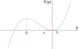
Figure 1: The cubic matrix model in the single-cut phase.

In the stable one-cut phase the eigenvalue density is supported on an interval $(a,b)$ around $p=0$: the spectral curve then takes the form

$$y(p)=M(p)\sqrt{(p-a)(p-b)},\qquad M(p)=g(p-p_{0})$$ (2.65)

where

$$p_{0}=-{1\over g}-{a+b\over 2}.$$ (2.66)

The branch points can be expressed as a function of the (only) ’t Hooft parameter by imposing the correct asymptotics for the planar resolvent [10], and one finds, as a power series in $t$,

$$\displaystyle a = 2\sqrt{t}-2gt+4g^{2}t^{3/2}-12g^{3}t^{2}+36g^{4}t^{5/2}-128g^{5}t^{3}+{\cal O}\left(t^{7/2}\right),$$

$$b = -2\sqrt{t}-2gt-4g^{2}t^{3/2}-12g^{3}t^{2}-36g^{4}t^{5/2}-128g^{5}t^{3}+{\cal O}\left(t^{7/2}\right).$$

It is now straightforward to compute $\beta$-deformed correlators from (2.39). For example, (2.54) gives

$$\displaystyle W_{0,1}(p) = -\frac{a(2b-3p+p_{0})-3bp+bp_{0}+4p^{2}-2pp_{0}}{4\sigma(p)(p-p_{0})}-\frac{\sqrt{(a-p_{0})(b-p_{0})}-2p+2p_{0}}{2(p-p_{0})\sqrt{\sigma(p)}}.$$

As an instance we have, up to order $t^{3}$ and $g^{7}$

$$\displaystyle\left\langle{\rm Tr}M^{3}\right\rangle = \frac{-4gt^{3}+\ldots}{g_{s}}+\left(1-\beta^{-1}\right)\left(9gt^{2}+118g^{3}t^{3}+\dots\right)$$ (2.68)

$$+ g_{s}\beta^{-1}\left(gt+28g^{3}t^{2}+664g^{5}t^{3}+\dots\right)$$

$$+ g_{s}(1-\beta^{-1})^{2}\left(\frac{6}{g}+17gt+182g^{3}t^{2}+2228g^{5}t^{3}+\dots\right)$$

$$+ g_{s}^{2}(1-\beta^{-1})\left(3g+198g^{3}t+6959g^{5}t^{2}+202254g^{7}t^{3}+\dots\right)+\dots$$

$$\left\langle{\rm Tr}M^{2}{\rm Tr}M\right\rangle^{(c)} = -4\left(gt^{2}+10g^{3}t^{3}+\ldots\right)+g_{s}\left(1-\beta^{-1}\right)\left(\frac{2}{g}+8gt+106g^{3}t^{2}+1640g^{5}t^{3}\right)+\dots$$

Example 2.4.

The quartic potential. Consider finally a potential of the form

$$V(x)={x^{2}\over 2}+gx^{4}.$$ (2.70)

The resolvent is given by [10]

$$W_{0}(z)={1\over 2}\Bigl{(}z+4gz^{3}-\bigl{(}1+8ga^{2}+4gz^{2}\bigr{)}{\sqrt{z^{2}-4a^{2}}}\Bigr{)},$$ (2.71)

where $a$ is a function of $g,t$

$$a^{2}={1\over 24g}\biggl{(}-1+{\sqrt{1+48gt}}\biggr{)}.$$ (2.72)

The moment function has two zeros at

$$z_{0}^{2}=-{1+8ga^{2}\over 4g},$$ (2.73)

and (2.54) gives [30]

$$W_{0,1}(z)=-{1\over 2}{z\over z^{2}-4a^{2}}+{3\over 2z\sqrt{1-4a^{2}/z^{2}}}+{\sqrt{1-4a^{2}/z_{0}^{2}\over 1-4a^{2}/z^{2}}}{z_{0}^{2}\over z(z^{2}-z_{0}^{2})}-{z\over z^{2}-z_{0}^{2}}.$$ (2.74)

This expression leads to explicit results for the enumeration of quadrangulations of the projective plane ${\mathbb{R}}{\mathbb{P}}^{2}$, see [30] for more details.

2.4 Two-cut examples

Let us now consider the two-cut case, where we have $s=2$. In this elliptic case there is one single integral $C_{1}(p)$ (2.48) to compute, and we can obtain very explicit expressions in terms of elliptic integrals [8]:

$$C_{1}(p) ={2\over\pi(p-x_{3})(p-x_{2}){\sqrt{(x_{1}-x_{3})(x_{2}-x_{4})}}}\biggl{[}(x_{2}-x_{3})\Pi(n_{4},k)+(p-x_{2})K(k)\biggr{]},$$ (2.75)

$$C^{\rm reg}_{1}(p) ={2\over\pi(p-x_{3})(p-x_{2}){\sqrt{(x_{1}-x_{3})(x_{2}-x_{4})}}}\biggl{[}(x_{3}-x_{2})\Pi(n_{1},k)+(p-x_{3})K(k)\biggr{]},$$

$$L_{1} =\frac{\pi\sqrt{(x_{1}-x_{3})(x_{2}-x_{4})}}{2K(k)},$$

where

$$k^{2}={(x_{1}-x_{2})(x_{3}-x_{4})\over(x_{1}-x_{3})(x_{2}-x_{4})},\qquad n_{4}={(x_{2}-x_{1})(p-x_{3})\over(x_{3}-x_{1})(p-x_{2})},\qquad n_{1}={(x_{4}-x_{3})(p-x_{2})\over(x_{4}-x_{2})(p-x_{3})},$$ (2.76)

$\Pi(n,k)$ is the elliptic integral of the third kind,

$$\Pi(n,k)=\int_{0}^{1}{{\rm d}t\over(1-nt^{2}){\sqrt{(1-t^{2})(1-k^{2}t^{2})}}}$$ (2.77)

and $K(k)$ is the standard elliptic integral of the second kind. The leading correction $W_{0,1}$ to the resolvent is given by (2.51). We will split the r.h.s as $W^{(A)}_{0,1}(p)+W^{(B)}_{0,1}(p)$, where

$$\displaystyle W^{(A)}_{0,1}(p) := -\frac{1}{4\pi{\rm i}{\sqrt{\sigma({p})}}}\oint_{\cal C}\frac{y^{\prime}(q){\rm d}q}{M(q)(p-q)},$$ (2.78)

$$W^{(B)}_{0,1}(p) := \frac{1}{4\pi{\rm i}{\sqrt{\sigma({p})}}}\left[\oint_{{\cal C}_{1}}\frac{C^{\rm reg}_{1}(q)L_{1}y^{\prime}(q){\rm d}q}{M(q)}+\oint_{{\cal C}_{2}}\frac{C_{1}(q)L_{1}y^{\prime}(q){\rm d}q}{M(q)}\right].$$ (2.79)

When $M(p)$ is a rational function of $p$, the integrand in (2.78) is a single valued meromorphic function outside the cuts and we can compute $W^{(A)}_{0,1}(p)$ by deforming the contour and picking up poles just as we did for the single cut case. On the other hand, as was pointed out in the discussion of Section 2.2, this is not the case for the expressions (2.75) for $C_{1}(p)$ and $C_{1}^{\rm reg}(p)$, which are only well-defined in the neighbourhood of the cuts $[x_{3},x_{4}]$ and $[x_{1},x_{2}]$ respectively. A way to treat the integrals appearing in (2.79) is the following: for a fixed polarization of the spectral curve, the elliptic modulus $k$ in (2.76) vanishes by definition when we shrink the $A$-cycle. By expanding the complete elliptic integrals $\Pi(n,k)$ and $K(k)$ appearing in (2.75) around $k=0$ and integrating term by term, we obtain an expansion of the form

$$W^{(B)}_{0,1}(p)=\frac{1}{4\pi{\rm i}{\sqrt{\sigma({p})}}}\sum_{n=0}^{\infty}\left[\oint_{{\cal C}_{1}}\frac{C^{[n],\rm reg}_{1}(q)L_{1}y^{\prime}(q){\rm d}q}{M(q)}+\oint_{{\cal C}_{2}}\frac{C^{[n]}_{1}(q)L_{1}y^{\prime}(q){\rm d}q}{M(q)}\right]k^{n},$$ (2.80)

where we denoted

$$f^{[n]}:=\frac{1}{n!}\frac{\partial^{n}f}{\partial k^{n}}\Bigg{|}_{k=0}.$$ (2.81)

At any fixed order in $k$, by formulae (A.40) and (A.39), the integrands of (2.80) are algebraic functions of $q$ as long as the moment function is rational, and can be computed exactly in terms of complete elliptic integrals.

It should be stressed that, while (2.80) yields only a perturbative expression valid for small $k$, this procedure holds true for a generic, fixed choice of polarization. It therefore provides a way to expand the amplitudes around any boundary point in the moduli space where the spectral curve develops a nodal singularity.

Example 2.5.

The cubic matrix model. As a first application of our formulae, let us consider the case of the cubic matrix model with

$$V(p)={p^{2}\over 2}+g{p^{3}\over 3}$$ (2.82)

in the two-cut case. The spectral curve reads

$$y(p)=M(p){\sqrt{\sigma({p})}},\quad M(p)=g,\quad\sigma(p)=\sqrt{(p-x_{1})(p-x_{2})(p-x_{3})(p-x_{4})}.$$ (2.83)

Following [13, 39] we can parametrize the branch points in terms of a pair of “B-model” variables ($z_{1}$, $z_{2}$) as

$$\sum_{i}x_{i}=2Q,\quad x_{2}-x_{1}=2\sqrt{z_{1}},\quad x_{4}-x_{3}=2\sqrt{z_{2}},\quad-x_{1}-x_{2}+x_{3}+x_{4}=2I$$ (2.84)

where

$$Q=-\frac{1}{g},\quad I=\sqrt{\frac{1}{g^{2}}-2(z_{1}+z_{2})}.$$ (2.85)

The ’t Hooft parameters can be computed explicitly in terms of complete elliptic integrals [33] as

$$\displaystyle t_{1} = \frac{(x_{4}-x_{3})(x_{2}-x_{4})(x_{1}-x_{4})^{2}}{\pi\sqrt{(x_{1}-x_{3})(x_{2}-x_{4})}}\Pi\left(\tilde{n}_{1},k\right),$$ (2.86)

$$t_{2} = \frac{(x_{4}-x_{2})(x_{2}-x_{1})(x_{3}-x_{2})^{2}}{\pi\sqrt{(x_{1}-x_{3})(x_{2}-x_{4})}}\Pi\left(\tilde{n}_{2},k\right),$$ (2.87)

where

$$k^{2}=\frac{(x_{1}-x_{2})(x_{3}-x_{4})}{(x_{1}-x_{3})(x_{2}-x_{4})},\quad\tilde{n}_{1}=\frac{x_{3}-x_{4}}{x_{3}-x_{1}},\quad\tilde{n}_{2}=\frac{x_{1}-x_{2}}{x_{1}-x_{3}}.$$ (2.88)

This can be inverted as

$$\displaystyle z_{1} = -4t_{1}+16g^{2}t_{1}^{2}-24g^{2}t_{1}t_{2}+\dots,$$ (2.89)

$$z_{2} = 4t_{2}-24g^{2}t_{1}t_{2}+16g^{2}t_{2}^{2}+\dots$$ (2.90)

Let us turn to compute $W^{(B)}_{0,1}(p)$ first. We can write it as

$$W^{(B)}_{0,1}(p)=\frac{I_{1}(t_{1},t_{2})+I_{2}(t_{1},t_{2})}{{\sqrt{\sigma({p})}}}$$ (2.91)

with

$$I_{j}=\sum_{n=0}^{\infty}\left[\oint_{A_{j}}\frac{C^{[n],\rm reg}_{1}(q)y^{\prime}(q)}{4\pi iM(q)L}\right]k^{n}.$$

We find

$$\displaystyle-I_{1} = \frac{1}{32}z_{1}\left(8g+24g^{3}z_{2}+81g^{5}z_{2}^{2}\right)+\frac{1}{64}z_{1}^{2}\left(20g^{3}+208g^{5}z_{2}+1269g^{7}z_{2}^{2}\right)+\dots$$

$$I_{2} = \left(\frac{gz_{2}}{4}+\frac{5g^{3}z_{2}^{2}}{16}\right)+z_{1}\left(\frac{3g^{3}z_{2}}{4}+\frac{13g^{5}z_{2}^{2}}{4}\right)+z_{1}^{2}\left(\frac{81g^{5}z_{2}}{32}+\frac{1269g^{7}z_{2}^{2}}{64}\right)+\dots$$

whereas the residue computation for $W^{(A)}_{0,1}(p)$ yields

$$W^{(A)}_{0,1}(p)=\frac{1}{4}\sum_{i=1}^{4}\frac{1}{x_{i}-p}+\frac{1+2gp}{2g{\sqrt{\sigma({p})}}}.$$ (2.93)

We can compare our result to explicit perturbative computations for the $\beta$-deformed cubic matrix model, along the lines of [40]. As an example, (2.91), (2.93) together yield up to quadratic order in $t_{1}$ and $t_{2}$

$$\displaystyle\left\langle{\rm Tr}M\right\rangle = \left(-\frac{t_{1}}{g}-gt_{1}^{2}-gt_{2}^{2}+4gt_{2}t_{1}+30g^{3}t_{2}^{2}t_{1}-30g^{3}t_{2}t_{1}^{2}-708g^{5}t_{2}^{2}t_{1}^{2}+\dots\right)g_{s}^{-1}$$

$$+ \left(1-\beta^{-1}\right)\left[g(t_{1}+t_{2})+g^{3}\left(9t_{2}^{2}-9t_{1}^{2}\right)+g^{5}\left(-162t_{1}^{2}t_{2}-162t_{1}t_{2}^{2}\right)+\dots\right]+\dots,$$

which perfectly agrees with the computation from perturbation theory.

Interestingly, a closed form expression for $W_{0,1}(p)$ can be found as a function of the branch points. It was shown in [35] that, for matrix models with constant moment function $M(p)=g$, $W_{0,1}$ is directly related to the planar resolvent as follows

$$W_{0,1}(p)=\partial_{t}W_{0}(p)-\frac{1}{4}\partial_{p}\ln\sigma(p).$$ (2.95)

The first term of the r.h.s. can be evaluated very explicitly upon expressing the derivative w.r.t. the total ’t Hooft coupling in terms of derivatives with respect to the branch points, following [48]. The partial derivatives $A_{i,j}=\frac{\partial x_{i}}{\partial t_{j}}$ satisfy the linear system

$$\displaystyle\sum_{i=1}^{4}M(x_{i})x_{i}^{k}A_{i,j} = 4\delta_{k,2},$$ (2.96)

$$\sum_{i=1}^{4}M(x_{i})K_{i}A_{i,j} = 4\pi\delta_{j,2},$$ (2.97)

where we denoted

$$K_{i}=\int_{x_{3}}^{x_{4}}\frac{{\sqrt{\sigma({p})}}}{p-x_{i}}.$$ (2.98)

As the $A_{i,j}$ are completely determined by (2.96)-(2.97), it is straightforward to perform explicitly the derivatives in (2.95) and obtain a compact expression for $W_{0,1}(p)$ as a function of the branch points. We get

$$W_{0,1}(p)=\frac{1}{{\sqrt{\sigma({p})}}}\Bigg{[}(x_{2}-x_{3})\frac{\Pi\left(\tilde{n}_{2},k\right)}{K\left(k\right)}-\frac{\pi\sqrt{(x_{1}-x_{3})(x_{2}-x_{4})}}{4K\left(k\right)}+p-x_{3}\Bigg{]}-\frac{\sigma^{\prime}(p)}{4\sigma(p)}.$$ (2.99)

It is worthwhile to remark that this expression has a more involved dependence on the branch points as compared to oriented, open string amplitudes at higher genus. The ordinary topological recursion [24, 27] prescribes the following general form for the $\beta=1$ correlators in the two-cut case

$$W_{g,0}(p_{1},\dots,p_{h})=\sum_{n=0}^{3g-3+2h}\left(\frac{E(k)}{K(k)}\right)^{n}f_{n}(\{x_{i}\},\{p_{j}\})=\sum_{n=0}^{3g-3+2h}\left(E_{2}(\tau)\right)^{n}\tilde{f}_{n}(\tau,\{p_{j}\})$$ (2.100)

where $\tau$ is the half-period ratio on the mirror curve, $\tilde{f}_{n}$ are holomorphic, weight $-2n$ modular forms for fixed $p_{j}$, and $E_{2}(\tau)$ is the second Eisenstein series (see [9, 12] for a detailed discussion). In particular, only first- and second-kind elliptic integrals are involved for $\beta=1$, whereas in the $\beta$-deformed case, as (2.99) shows, we have a more sophisticated dependence on closed string moduli due to the appearance of elliptic integrals of the third kind at prescribed values for the elliptic characteristic. It would be interesting to track the origin of this higher degree of complexity for $\beta$-deformed amplitudes.

Example 2.6.

The symmetric double-well. As the simplest instance of a two-cut model with non-trivial moment function, consider the double well potential

$$V(p)=-{p^{2}\over 2}+g{p^{4}\over 4},$$ (2.101)

depicted in Fig. 2.

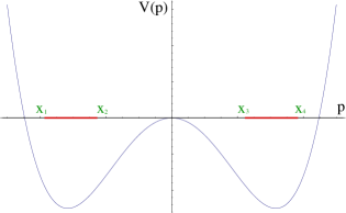
Figure 2: The double-well potential in the symmetric 2-cut phase.

The potential has two minima at $p=\pm 1/\sqrt{g}$ and a maximum at $p=0$. For simplicity we consider the case in which we equally distribute the eigenvalues between the two minima, i.e. we restrict to the symmetric slice $t_{1}=t_{3}=t/2$, $t_{2}=0$. The moment function in this case takes the form

$$M(p)=gp.$$ (2.102)

The branch points can be readily computed as a function of the total ’t Hooft coupling $t$ by imposing the $\mathbb{Z}_{2}$ symmetry between the cuts and the leading asymptotics of the resolvent. We get

$$x_{1}=-\sqrt{\frac{1}{g}+\frac{2\sqrt{t}}{\sqrt{g}}},\quad x_{2}=-\sqrt{\frac{1}{g}-\frac{2\sqrt{t}}{\sqrt{g}}},\quad x_{3}=\sqrt{\frac{1}{g}-\frac{2\sqrt{t}}{\sqrt{g}}},\quad x_{4}=\sqrt{\frac{1}{g}+\frac{2\sqrt{t}}{\sqrt{g}}}.$$ (2.103)

We now turn to compute $W^{(B)}_{0,1}(p)$. In this case, the integrals in (2.79) can be computed exactly. To see this, let us consider the $PSL(2,\mathbb{C})$ transformation

$$p\to\tilde{p}=\frac{\alpha p+\beta}{\gamma p+\delta},\quad A=\left(\begin{array}[]{ll}\alpha&\beta\\ \gamma&\delta\end{array}\right)\in PSL(2,\mathbb{C})$$ (2.104)

with

$$\alpha =-\delta=\left(x_{4}x_{1}-x_{2}x_{3}\right)\zeta,$$ (2.105)

$$\beta =(x_{1}x_{2}x_{3}-x_{1}x_{3}x_{4}+x_{2}x_{3}x_{4}-x_{1}x_{2}x_{4})\zeta,$$

$$\gamma =(x_{1}+x_{4}-x_{2}-x_{3})\zeta.$$

In these equations, $\zeta$ is given by

$$\zeta:=\frac{(x_{4}-x_{1})}{(x_{1}-x_{3})\sqrt{(x_{1}-x_{4})(x_{1}-x_{2})(x_{2}-x_{4})(x_{3}-x_{4})}}.$$ (2.106)

Let us apply this transformation to the second integral on the r.h.s. of (2.79). Then the sum of the two integrals becomes the single definite integral

$$\oint_{{\cal C}_{1}}\frac{{\rm d}q}{4\pi{\rm i}}\left[\left(\frac{y^{\prime}(\tilde{q})}{M(\tilde{q})}+\frac{y^{\prime}(q)}{M(q)}\right)C_{1}^{\rm reg}(q)L_{1}+\frac{(x_{1}-x_{2}-x_{3}+x_{4})y^{\prime}(\tilde{q})}{(x_{1}(x_{4}-q)+(x_{3}-x_{4})q+x_{2}(q-x_{3}))M(\tilde{q})}\right].$$ (2.107)

In the case of the symmetric double-well, (2.103) implies

$$\frac{y^{\prime}(\tilde{q})}{M(\tilde{q})}=-\frac{y^{\prime}(q)}{M(q)},\quad x_{1}+x_{4}-x_{2}-x_{3}=0,$$ (2.108)

therefore

$$W^{(B)}_{0,1}(p)=0.$$ (2.109)

For $W^{(A)}_{0,1}(p)$ we instead find

$$W^{(A)}_{0,1}(p)=\frac{\sqrt{1-4t}+3gp^{2}}{2pg{\sqrt{\sigma({p})}}}+\frac{-3g^{2}p^{4}+g\left(4p^{2}+4t\right)-1}{2pg^{2}\sigma(p)}.$$ (2.110)

As an example, this yields

$$\left\langle{\rm Tr}M^{4}\right\rangle_{0,1}=\frac{1}{g^{2}}-\frac{2t}{g}-t^{2}-2gt^{3}-5g^{2}t^{4}-14g^{3}t^{5}+{\cal O}(g^{4}).$$ (2.111)

3 Applications to supersymmetric gauge theories

3.1 Superpotentials in ${\cal N}=1$ gauge theories

In [19, 20] Dijkgraaf and Vafa argued that superpotentials in a large class of ${\cal N}=1$ supersymmetric gauge theories can be computed by using matrix models. Let us consider an ${\cal N}=1$ supersymmetric gauge theory with gauge group $G={\rm U}(N),{\rm SO}(N)$ or ${\rm Sp}(N)$, where the superfield strength is denoted by ${\cal W}^{\alpha}$. There is also a chiral superfield $\Phi$ in a representation $R$ of the gauge group $G$, with a tree level superpotential $W_{\rm tree}(\Phi)$, which we will assume to be a polynomial of degree $d$:

$$W_{\rm tree}(\Phi)=\sum_{j=1}^{d}{g_{j}\over j}{\rm Tr}\Phi^{j}.$$ (3.1)

If all roots of $W^{\prime}_{\rm tree}(x)=g_{d}\prod_{i=1}^{d-1}(x-a_{i})$ are distinct, the matter fields are all massive; a classical vev for $\Phi$, where $N_{i}$ of its eigenvalues are equal to $a_{i}$, spontaneously breaks part of the gauge symmetry, and the massive fields can be integrated out to get an effective action for the unbroken gauge degrees of freedom at low energy.

Depending on the gauge group and the representation we will end up with different patterns of gauge symmetry breaking (see the useful summary in eq. (2.1) of [35])). We will be particularly interested in the examples where $G={\rm SO}(N),\,{\rm Sp}(N)$ and $R$ is, respectively, the symmetric and the antisymmetric representation of the group. In this case, we have the simple patterns of gauge symmetry breaking

$${\rm SO}(N)\rightarrow \prod_{i=1}^{k}{\rm SO}(N_{i}),$$ (3.2)

$${\rm Sp}(N)\rightarrow \prod_{i=1}^{k}{\rm Sp}(N_{i}),$$

where $1\leq k\leq d-1$, and there will be, correspondingly, various gluino superfields for the unbroken gauge groups,

$$S_{i}=-{1\over 32\pi}{\rm Tr}\left({\cal W}^{(i),\,\alpha}{\cal W}^{(i)}_{\alpha}\right),$$ (3.3)

where ${\cal W}^{(i)}_{\alpha}$ is the superfield strength for the $i$-th gauge group. According to the proposal of [19, 20], the effective superpotential for the glueball superfields, as well as the gauge coupling matrix for the infrared-free abelian fields, should be computable from an auxiliary matrix model with $V(x)=W_{\rm tree}(x)$. In particular, the glueball superpotential, as a function of the gluino superfields, is given by [37, 43, 35]

$$W_{\rm eff}(S_{i})=W_{\rm VY}(S_{i})+\sum_{i=1}^{k}N_{i}{\partial F_{0,0}\over\partial S_{i}}-4\epsilon F_{0,1}$$ (3.4)

where $\epsilon=\pm 1$ for ${\rm SO}/{\rm Sp}$, respectively and $W_{\rm VY}(S_{i})$ is the Veneziano–Yankielowicz superpotential (see [35] for a detailed expression). In this equation, $F_{0,0}$, $F_{0,1}$ are the first two free energies in the expansion (2.3), obtained in the $\beta$-ensemble for a matrix model with potential $V(x)=W_{\rm tree}(x)$, in the $k$-cut phase, and with ’t Hooft parameters $S_{i}$. In addition, the gauge theory quantity

$$T(z)=\left\langle{\rm Tr}\left({1\over z-\Phi}\right)\right\rangle$$ (3.5)

can be computed from the generalized Konishi anomaly [3] and expressed in terms of matrix model resolvents [42, 35]:

$$T(z)=\sum_{i=1}^{k}N_{i}{\partial W_{0,0}(z)\over\partial S_{i}}-4\epsilon W_{0,1}(z),$$ (3.6)

where again $\epsilon=\pm 1$ for ${\rm SO}/{\rm Sp}$. Similarly, contributions to chiral ring observables induced by a non-flat gravity background can be computed in terms of non-planar corrections to the resolvent [4].

The formulae above for the solution of (2.39) in the polynomial matrix model case give then explicit results for computing a large class of vevs of chiral observables for a general $W_{\rm tree}(x)$. In particular, $W_{0,1}$ and $F_{0,1}$ yield the unoriented contribution to the the effective superpotential (3.4) and gauge theory resolvent (3.6) for a general tree-level superpotential. As an example and a test of our computations, let us consider the case of classically unbroken gauge symmetry, where $k=1$. This corresponds to the one-cut case in the computations above. Using the well-known one-cut result (see for example [18])

$${\partial W_{0,0}(z)\over\partial z}={1\over{\sqrt{\sigma(z)}}},$$ (3.7)

as well as (2.53), we find the general formula

$$T(z)={N\over{\sqrt{\sigma(z)}}}+{2\epsilon}{y^{\prime}(z)\over y(z)}-{2\epsilon\over{\sqrt{\sigma(z)}}}\left[d-1+\sum_{i}{\sqrt{\sigma(z_{i})}\over p-z_{i}}\right].$$ (3.8)

This agrees with the explicit computation for the quartic potential in [3].

3.2 Penner model and AGT correspondence

A more sophisticated example is given by the double Penner model

$$V(x)=\alpha_{1}\log x+\alpha_{2}\log(x-1).$$ (3.9)

This model was recently considered by Dijkgraaf and Vafa [21] in the context of the AGT correspondence [5], where it was shown to give a matrix model representation of the chiral three-point function in Liouville theory; its 4d counterpart arises [29] as the dimensional reduction of the 6d $A_{1}$ (2,0) theory compactified on a sphere with three punctures, and is a $U(1)$ theory with four hypermultiplets. The spectral curve for this case reads

$$M(p){\sqrt{\sigma({p})}}=\frac{\sqrt{\alpha_{1}^{2}(1-p)+\alpha_{3}^{2}(p^{2}-p)+\alpha_{2}^{2}p}}{p(p-1)}$$ (3.10)

where $\alpha_{3}=-t-\alpha_{1}-\alpha_{2}$ and $t=g_{s}N$.

An extension of the AGT correspondence in presence of defects was considered in [6], where multiple insertions of surface operators on the 4d gauge theory side were mapped to insertions of vertex operators corresponding to degenerate states on the Liouville theory side. In [41, 22] both were mapped in turn to $A$-type open topological string amplitudes on the toric geometries that engineer the relevant gauge theory. In particular the authors of [41] conjectured and checked that the Liouville theory four–point function with one degenerate insertion and vanishing background charge $Q=b+1/b$

$$Z_{\rm null}(p,\hbar,b=i)=\frac{\left\langle\frac{\alpha_{1}}{\hbar}|V_{-\alpha_{2}/\hbar}(1)V_{-b/2}(p)|-\frac{\alpha_{3}}{\hbar}+\frac{b}{2}\right\rangle}{\left\langle\frac{\alpha_{1}}{\hbar}|V_{-\alpha_{2}/\hbar}(1)|-\frac{\alpha_{3}}{\hbar}\right\rangle}\Bigg{|}_{b={\rm i}}\,,$$ (3.11)

should be expressible in terms of oriented topological string amplitudes computed through the Eynard-Orantin recursion applied to (3.10)

$$Z_{\rm null}(p,\hbar,b=i)=\exp\left[\frac{1}{\hbar}A_{1}^{(0)}(p)+\frac{1}{2!}A_{2}^{(0)}(p,p)+\hbar\left(A_{1}^{(1)}(p)+\frac{1}{3!}A^{(0)}_{3}(p,p,p)\right)+\dots\right],$$ (3.12)

with

$$A_{h}^{(g)}(p_{1},\dots,p_{h})=\int{\rm d}p_{1}\dots\rm dp_{h}W_{h}^{(g)}(p_{1},\dots,p_{h}).$$ (3.13)

On the other hand, it was proposed in [21] that turning on a background charge $Q$ on the CFT side should exactly correspond to the $\beta$-deformation of the matrix model, with the dictionary been given by

$$Q^{2}=-\gamma^{2},\quad b^{2}=-\beta,\quad\hbar=\frac{g_{s}}{\sqrt{\beta}}.$$ (3.14)

This was checked by direct computation in [55, 49, 50, 38] at the level of the free energy. It is therefore tempting to look at a combination of the two claims above and compute refined open string amplitudes via (2.39), corresponding to degenerate insertions in Liouville theory with non-vanishing $Q$. A natural extension of (3.12) in the $\beta$-deformed case is through an expansion of the form

$$F_{\rm null}(p,\hbar,b) =\log Z_{\rm null}(p,\hbar,b)$$ (3.15)

$$=\sum_{n=-1}\left(\sqrt{\beta}\hbar\right)^{n}\sum_{g,h,k|2g-2+h+k=n}\frac{1}{h!}\beta^{1-g-k/2}A^{(g)}_{h,k}(p,\cdots p)\gamma^{k}.$$

The $\beta$-deformed topological recursion allows us to test this proposal in detail. On the CFT side it is well-known that Ward identities for the normalized four point function (3.11) reduce to a hypergeometric differential equation; more precisely we have that

$$Z_{\rm null}(p,\hbar,b)=p^{\frac{b\alpha_{1}}{\hbar}}(1-p)^{\frac{-b\alpha_{2}}{\hbar}}\,{}_{2}F_{1}(A_{1},A_{2};B_{1};p)\,,$$ (3.16)

where

$$A_{1}=b\,\frac{\alpha_{3}-\alpha_{2}+\alpha_{1}}{\hbar}\,,\qquad A_{2}=b\,\left(\frac{\alpha_{1}-\alpha_{2}-\alpha_{3}}{\hbar}+Q\right)\,,\qquad B_{1}=\frac{2b\alpha_{1}}{\hbar}\,.$$ (3.17)

By Taylor expanding around $\hbar=0$, $b=i$ we obtain

$$\displaystyle\log Z_{\rm null}(p) = \frac{b}{\hbar}A^{(0)}_{1,0}(p)+\left[-\frac{b^{2}}{2}A^{(0)}_{2,0}(p,p)+(b^{2}+1)A^{(0)}_{1,1}(p)\Big{)}\right]$$

$$+ \frac{\hbar}{2b}\left[(1+b^{2})^{2}A^{(0)}_{1,2}(p)-b^{2}(b^{2}+1)\frac{1}{2}A^{(0)}_{2,1}(p,p)-b^{2}A^{(1)}_{1,0}(p)+b^{4}\frac{1}{3!}A^{(0)}_{3,0}(p,p,p)\right]$$

$$+ \frac{\hbar^{2}}{4b^{2}}\Bigg{[}(b^{2}+1)^{3}A^{(0)}_{1,3}(p)-b^{2}(1+b^{2})A^{(1)}_{1,1}(p)+b^{4}\frac{1}{2}A^{(1)}_{2,0}(p,p)-(1+b^{2})$$

$$b^{2}\frac{1}{2}A^{(0)}_{2,2}(p,p)-b^{6}\frac{1}{4!}A^{(0)}_{4,0}(p,p,p,p)+\frac{1}{3!}b^{4}(b^{2}+1)A^{(0)}_{3,1}(p,p,p)\Bigg{]}+\mathcal{O}\left(\frac{\hbar}{b}\right)^{3}.$$

On the other hand, we can apply the refined recursion to the spectral curve (3.10). In this case, the contour integrals also have contributions from the poles of $M(x)$; as an instance, we find for the one-crosscap correction to the resolvent

$$W_{0,1}(p)=-{1\over 2}{y^{\prime}(p)\over y(p)}+{1\over 2{\sqrt{\sigma(p)}}}\sum_{i=1}^{3}{\rm Res}_{z=z_{i}}\left[{1\over p-z}\left({M^{\prime}(z)\over M(z)}\sqrt{\sigma(z)}+{1\over 2}{2z-a-b\over{\sqrt{\sigma(z)}}}\right)\right],$$ (3.19)

where

$$z_{1}=0,\quad z_{2}=1,\quad z_{3}=\infty.$$ (3.20)

The residues give the values

$$-{\alpha_{1}\over\alpha_{0}}{1\over p},\qquad-{\alpha_{2}\over\alpha_{0}}{1\over p-1},\qquad-1,$$ (3.21)

for $i=1,2,3$, respectively, and we finally obtain

$$W_{0,1}(p)=-{1\over 2}{M^{\prime}(p)\over M(p)}-{1\over 4}{2p-a-b\over(p-a)(p-b)}-{1\over 2{\sqrt{\sigma(p)}}}\left(1+{\alpha_{1}\over\alpha_{0}}{1\over p}+{\alpha_{2}\over\alpha_{0}}{1\over p-1}.\right).$$ (3.22)

The integrated refined amplitudes $A^{(g)}_{h,k}(p,\cdots p)$ can be similarly computed in a straightforward fashion from (2.39); upon taking into account the dictionary (3.14), we find exact agreement with the CFT expansion (LABEL:eq:cftexp).

4 The $\beta$-deformed Chern–Simons matrix model

4.1 Definition and relation to the Stieltjes–Wigert ensemble

The $\beta$-deformed Chern–Simons (CS) matrix model on ${\mathbb{S}}^{3}$ is defined by the partition function

$$Z_{\rm CS}(N,g_{s},\beta)={1\over N!}\int\prod_{i=1}^{N}{{\rm d}x_{i}\over 2\pi}{\rm e}^{-{\beta\over 2g_{s}}\sum_{i=1}^{n}x_{i}^{2}}\prod_{i<j}\left(2\sinh{x_{i}-x_{j}\over 2}\right)^{2\beta}.$$ (4.1)

When $\beta=1$ we recover the standard CS matrix model considered in [45, 46]. This generalization of the CS matrix model is the natural counterpart of the $\beta$-ensemble deformation of the standard Hermitian matrix model.

In [58] Tierz pointed out that the standard CS matrix model could be written in the usual, Hermitian form, i.e. with a Vandermonde inteaction among eigenvalues, but with a potential

$$V(x)={1\over 2}\left(\log x\right)^{2}.$$ (4.2)

This potential defines the so-called Stieltjes–Wigert (SW) matrix model. It is very easy to show that (4.1) is, up to a simple multiplicative factor, the partition function of the $\beta$-deformed version of the SW matrix model. To do that, we perform the change of variables

$$u_{i}=c\,{\rm e}^{x_{i}}$$ (4.3)

where $c$ is given by

$$c=\exp\left(t-g_{s}(1-\beta^{-1})\right),\qquad t=g_{s}N.$$ (4.4)

A simple computation shows that

$$Z_{\rm CS}(N,g_{s},\beta)={\rm e}^{-{\beta N\over 2g_{s}}(\log c)^{2}}Z_{\rm SW}(N,g_{s},\beta)$$ (4.5)

where

$$Z_{\rm SW}(N,g_{s},\beta)={1\over N!}\int\prod_{i=1}^{N}{{\rm d}u_{i}\over 2\pi}{\rm e}^{-{\beta\over 2g_{s}}\sum_{i=1}^{n}(\log u_{i})^{2}}\prod_{i<j}\left(u_{i}-u_{j}\right)^{2\beta}$$ (4.6)

is the partition function of the $\beta$-deformed SW ensemble. In terms of free energies we have

$$F_{\rm CS}(N,g_{s},\beta)=-{\beta t^{3}\over 2}g_{s}^{-2}+g_{s}^{-1}(\beta-1)t^{2}-(\beta+\beta^{-1}-2){t\over 2}+F_{\rm SW}(N,\beta,g_{s}).$$ (4.7)

The change of variables (4.3) has to be taken into account when computing correlation functions in the CS matrix model from the SW matrix model, and we have the relationship

$$\langle{\rm Tr}\,U^{n}\rangle^{\rm SW}=\exp\left(nt-ng_{s}(1-\beta^{-1})\right)\langle{\rm Tr}\,{\rm e}^{nX}\rangle^{\rm CS},$$ (4.8)

where

$$U={\rm diag}(u_{1},\cdots,u_{N}),\quad X={\rm diag}(x_{1},\cdots,x_{N}).$$ (4.9)

It was shown in [46] that, though both the potential (4.2) and its first derivative are non-polyomial, the SW model can be solved at large $N$ with standard saddle-point techniques. In particular, the resolvent is given by

$$W_{0}(p)=-{1\over p}\log\left[{1+{\rm e}^{-t}p+{\sqrt{(1+{\rm e}^{-t}p)^{2}-4p}}\over 2p}\right],$$ (4.10)

and the spectral curve is

$$y(p)=M(p){\sqrt{(p-a)(p-b)}}={2\over p}\tanh^{-1}\left[{{\sqrt{(1+{\rm e}^{-t}p)^{2}-4p}}\over 1+{\rm e}^{-t}p}\right],$$ (4.11)

where

$$M(p)={2\over p{\sqrt{(p-a)(p-b)}}}\tanh^{-1}\left[{{\sqrt{(1+{\rm e}^{-t}p)^{2}-4p}}\over 1+{\rm e}^{-t}p}\right]$$ (4.12)

and the positions of the endpoints are given by

$$a(t) = 2{\rm e}^{2t}-{\rm e}^{t}+2{\rm e}^{3t\over 2}{\sqrt{{\rm e}^{t}-1}},$$

$$b(t) = 2{\rm e}^{2t}-{\rm e}^{t}-2{\rm e}^{3t\over 2}{\sqrt{{\rm e}^{t}-1}}.$$ (4.13)

For $t=0$, $a(0)=b(0)=1$, which is indeed the minimum of (4.2).

4.2 Corrections to the resolvent and to the free energy

The SW ensemble is, from many points of view, a conventional one-cut matrix model, and its correlation functions and free energies obey the standard recursion relations of [27, 15]. We now proceed to calculate the first $\beta$-deformed corrections to the resolvent and the free energy by using the recursion of [15].

Let us first consider the correction fo the 1-point correlator (2.51). As in the standard polynomial case, there is no contribution from $V^{\prime\prime}(q)$ (since both this function and $M(q)$ are analytic on the cut). In order to proceed, it will be useful to change variables from $q$ to $\zeta$ through,

$$q={b-a\over 2}\zeta+{a+b\over 2}.$$ (4.14)

This maps the interval $[a,b]$ to $[-1,1]$. Explicitly,

$$q=2{\rm e}^{t}\sqrt{{\rm e}^{t}({\rm e}^{t}-1)}\zeta+{\rm e}^{t}\left(2{\rm e}^{t}-1\right).$$ (4.15)

In terms of $\zeta$ we have

$$\tanh^{-1}\left[{{\sqrt{(1+{\rm e}^{-t}q)^{2}-4q}}\over 1+{\rm e}^{-t}q}\right]=\tanh^{-1}\left({{\sqrt{\zeta^{2}-1}}\over\zeta+(1-{\rm e}^{-t})^{-1/2}}\right),$$ (4.16)

and the moment function reads

$$M(\zeta)={1\over\left(c_{1}+c_{2}\zeta\right)\sqrt{\zeta^{2}-1}}\tanh^{-1}\left({{\sqrt{\zeta^{2}-1}}\over\zeta+(1-{\rm e}^{-t})^{-1/2}}\right),$$ (4.17)

where

$$c_{1}={\rm e}^{5t/2}\sqrt{{\rm e}^{t}-1}\left(2{\rm e}^{t}-1\right),\quad c_{2}=2{\rm e}^{3t}\left({\rm e}^{t}-1\right).$$ (4.18)

The integrand of (2.51) involves then,

$$-{1\over 2}{\rm d}p{y^{\prime}(q)\over M(q)}={1\over 2q}{\sqrt{(q-a)(q-b)}}{\rm d}q-{\rm e}^{t}{\cal M}(\zeta){\rm d}\zeta,$$ (4.19)

with

$${\cal M}(\zeta)={{\sqrt{{\rm e}^{t}({\rm e}^{t}-1)}}\left(\sqrt{{\rm e}^{t}({\rm e}^{t}-1)}\zeta+{\rm e}^{t}-1\right)\over\left(2\sqrt{{\rm e}^{t}({\rm e}^{t}-1)}\zeta+2{\rm e}^{t}-1\right)\tanh^{-1}\left({{\sqrt{\zeta^{2}-1}}\over\zeta+(1-{\rm e}^{-t})^{-1/2}}\right)}.$$ (4.20)

We then obtain,

$$W_{0,1}(p)={1\over 2}{p-{\rm e}^{t}\over p{\sqrt{\sigma(p)}}}-{1\over 2p}-{{\rm e}^{t}\over{\sqrt{\sigma(p)}}}\oint_{{\cal C}}{{\cal M}(\zeta)\over p-2{\rm e}^{t}\sqrt{{\rm e}^{t}({\rm e}^{t}-1)}\zeta-{\rm e}^{t}\left(2{\rm e}^{t}-1\right)}{{\rm d}\zeta\over 2\pi{\rm i}},$$ (4.21)

where the integral involving the first term in (4.19) has been calculated through a contour deformation and picking residues at $q=0,\infty,p$, and the contour ${\cal C}$ encircles the cut $[-1,1]$ in the $\zeta$ variable.

We have not been able to calculate the second term in (4.21) in closed form. In order to obtain explicit results, we have to perform a series expansion in both $p$ and $t$. To see an explicit example of this procedure, we expand around $p=\infty$ to obtain

$$W_{0,1}(p)\Big{|}_{p^{-2}}=-{\rm e}^{t}({\rm e}^{t}-1)+{\rm e}^{t}S(t)$$ (4.22)

where

$$S(t)={1\over\pi{\rm i}}\int_{-1}^{1}{\rm d}\zeta\,{\cal M}(\zeta).$$ (4.23)

Notice that this integral depends on $t$ only through the variable $\nu={\rm e}^{t}$. It can be computed systematically as a power series in $\nu-1$, which can then be re-expanded as a power series in $t$. We obtain, for the first few orders,

$$S(t)=-\frac{t}{2}-\frac{7t^{2}}{24}-\frac{71t^{3}}{720}-\frac{2971t^{4}}{120960}-\frac{17809t^{5}}{3628800}-\frac{4843t^{6}}{5913600}-\frac{51012187t^{7}}{435891456000}+{\cal O}\left(t^{8}\right).$$ (4.24)

The planar limit of the vev of ${\rm Tr}\,U$ is given by

$$\langle{\rm Tr}\,U\rangle^{\rm SW}_{0,0}={\rm e}^{t}({\rm e}^{t}-1),$$ (4.25)

and its first correction is given by (4.22),

$$\langle{\rm Tr}U\rangle^{\rm SW}_{0,1}=W_{0,1}(p)\bigg{|}_{p^{-2}}={\rm e}^{t}\left(S(t)-{\rm e}^{t}+1\right).$$ (4.26)

Together with (4.8) we then deduce that

$$\langle{\rm Tr}\,{\rm e}^{x}\rangle^{\rm CS}_{0,1}=S(t).$$ (4.27)

On the other hand, a direct perturbative computation of the vev $\langle{\rm Tr}\,{\rm e}^{x}\rangle^{\rm CS}$ in the CS matrix model (4.1) gives

$$\langle{\rm Tr}\,{\rm e}^{x}\rangle^{\rm CS} =N+g_{s}\left[{N^{2}\over 2}-{1\over 2}(1-\beta^{-1})N\right]$$ (4.28)

$$+g_{s}^{2}\left[{N^{3}\over 6}-{7\over 24}(1-\beta^{-1})N^{2}-{1\over 24}\beta^{-1}N+{1\over 8}(1-\beta^{-1})^{2}N\right]$$

$$+g_{s}^{3}\biggl{[}{N^{4}\over 24}-{71\over 720}N^{3}(1-\beta^{-1})-{1\over 48}\beta^{-1}N^{2}+{7\over 90}(1-\beta^{-1})^{2}N^{2}$$

$$-{1\over 48}(1-\beta^{-1})^{3}N+{11\over 720}\beta^{-2}(\beta-1)N\biggr{]}+{\cal O}(g_{s}^{4}),$$

in complete agreement with (4.27).

Using the same type of techniques we can also compute the first correction to the free energy. Using (2.56) we find,

$$\partial_{t}F^{\rm SW}_{0,1}=1+\int_{a}^{b}{{\rm d}p\over\pi}{\log|M(p)|\over{\sqrt{|\sigma(p)|}}}+\int_{a}^{b}{{\rm d}p\over 2\pi}{\log|\sigma(p)|\over{\sqrt{|\sigma(p)|}}}.$$ (4.29)

The last integral can be computed exactly:

$$\int_{a}^{b}{{\rm d}p\over 4\pi}{\log|\sigma(p)|\over{\sqrt{|\sigma(p)|}}}=\frac{\log(1-{\rm e}^{-t})}{2}+2t.$$ (4.30)

The first integral can be written, using again the change of variables (4.14), as

$$\int_{a}^{b}{{\rm d}p\over\pi}{\log|M(p)|\over{\sqrt{|\sigma(p)|}}}=\int_{-1}^{1}{{\rm d}\zeta\over\pi}\frac{1}{\sqrt{1-\zeta^{2}}}\log\left(\frac{\tan^{-1}\left(\frac{\sqrt{1-\zeta^{2}}}{\zeta+\frac{1}{\sqrt{1-e^{-t}}}}\right)}{\left(c_{1}+c_{2}\zeta\right)\sqrt{1-\zeta^{2}}}\right),$$ (4.31)

where $c_{1}$, $c_{2}$ are defined in (4.18). As before, this integral can be computed as a power series in $t$ around $t=0$. Putting everything together, and taking into account (4.7), we find

$$F^{\rm CS}_{0,1}(t)=\frac{1}{2}(\log(t)+1)t-\frac{t^{2}}{12}+\frac{t^{3}}{1440}+\frac{17t^{4}}{45360}-\frac{137t^{5}}{14515200}-\frac{2t^{6}}{467775}+{\cal O}(t^{7}).$$ (4.32)

We have again verified the very first coefficients in this expansion against a direct perturbative calculation in the CS matrix model.

It is worth pointing out that the corrections appearing in the CS matrix model when $\beta\not=1$ are much more complicated than the “standard” ones. For example, for $\beta=1$ all the correlators are polynomials in ${\rm e}^{t}$, while the integral giving (4.23) is not.

4.3 $\beta$-deformation and the $\Omega$ background

One of the interesting aspects of the conventional CS matrix model with $\beta=1$ is that its large $N$ expansion equals the $1/N$ expansion of topological string theory on the resolved conifold [31], since it equals the partition function of CS theory on the three-sphere. On the other hand, the partition function of topological string theory on the resolved conifold admits a refinement given by the K-theoretic version of Nekrasov’s partition function for a $U(1)$ theory [54]. This partition function can be also obtained from the refined topological vertex of [36]. The first correction to the refined free energy of the resolved conifold is simply

$$F_{0,1}^{\rm ref}={1\over 2}{\rm Li}_{2}({\rm e}^{-t}).$$ (4.33)

This expression is much simpler than the result (4.32).

We can also compare the result for $\langle{\rm Tr}\,{\rm e}^{x}\rangle^{\rm CS}$ with expectations coming from the theory of the refined vertex. When $\beta=1$, the correlation function $\langle{\rm Tr}\,{\rm e}^{x}\rangle^{\rm CS}$ can be expressed in terms of the open string amplitude

$$Z_{\vbox{\offinterlineskip\kern 1.0pt\hbox{\kern 1.0pt\vbox{\hbox{\vbox{\hbox{\vbox to0.0pt{\hrule height=0.4pt,width=3.90555pt\vss}}\hbox{\vbox{\hbox to0.0pt{\vrule width=0.4pt,height=3.90555pt\hss}}\kern 3.90555pt\vbox{\hbox to0.0pt{\vrule width=0.4pt,height=3.90555pt\hss}}}\hbox{\vbox{\hbox{\vbox to0.0pt{\hrule height=0.4pt,width=4.30554pt\vss}}}\kern-0.4pt}}}\hbox{} }\kern 1.0pt\kern 0.4pt}\kern 1.0pt\kern 0.4pt}}(t,g_{s})={1-Q\over 2\sinh\left({g_{s}\over 2}\right)}.$$

for a D-brane in an external leg of the resolved conifold. Here, $Q={\rm e}^{-t}$. The precise relation involves a framing factor,

$$\langle{\rm Tr}\,{\rm e}^{x}\rangle^{\rm CS}_{\beta=1}={\rm e}^{t}Z_{\vbox{\offinterlineskip\kern 1.0pt\hbox{\kern 1.0pt\vbox{\hbox{\vbox{\hbox{\vbox to0.0pt{\hrule height=0.4pt,width=3.90555pt\vss}}\hbox{\vbox{\hbox to0.0pt{\vrule width=0.4pt,height=3.90555pt\hss}}\kern 3.90555pt\vbox{\hbox to0.0pt{\vrule width=0.4pt,height=3.90555pt\hss}}}\hbox{\vbox{\hbox{\vbox to0.0pt{\hrule height=0.4pt,width=4.30554pt\vss}}}\kern-0.4pt}}}\hbox{} }\kern 1.0pt\kern 0.4pt}\kern 1.0pt\kern 0.4pt}}(t,g_{s}).$$ (4.34)

The “refined” version of the D-brane amplitude is

$$Z_{\vbox{\offinterlineskip\kern 1.0pt\hbox{\kern 1.0pt\vbox{\hbox{\vbox{\hbox{\vbox to0.0pt{\hrule height=0.4pt,width=3.90555pt\vss}}\hbox{\vbox{\hbox to0.0pt{\vrule width=0.4pt,height=3.90555pt\hss}}\kern 3.90555pt\vbox{\hbox to0.0pt{\vrule width=0.4pt,height=3.90555pt\hss}}}\hbox{\vbox{\hbox{\vbox to0.0pt{\hrule height=0.4pt,width=4.30554pt\vss}}}\kern-0.4pt}}}\hbox{} }\kern 1.0pt\kern 0.4pt}\kern 1.0pt\kern 0.4pt}}(t,g_{s},\beta)=\frac{Q\sqrt{q_{2}}-\sqrt{q_{1}}}{q_{2}-1}$$ (4.35)

with

$$q={\rm e}^{-\sqrt{\beta}g_{s}},\quad t={\rm e}^{-g_{s}/\sqrt{\beta}}.$$ (4.36)

Expanding in $g_{s}$ and $\beta$ we obtain

$$Z_{\vbox{\offinterlineskip\kern 1.0pt\hbox{\kern 1.0pt\vbox{\hbox{\vbox{\hbox{\vbox to0.0pt{\hrule height=0.4pt,width=3.90555pt\vss}}\hbox{\vbox{\hbox to0.0pt{\vrule width=0.4pt,height=3.90555pt\hss}}\kern 3.90555pt\vbox{\hbox to0.0pt{\vrule width=0.4pt,height=3.90555pt\hss}}}\hbox{\vbox{\hbox{\vbox to0.0pt{\hrule height=0.4pt,width=4.30554pt\vss}}}\kern-0.4pt}}}\hbox{} }\kern 1.0pt\kern 0.4pt}\kern 1.0pt\kern 0.4pt}}(t,g_{s},\beta)=\left(1-{\rm e}^{-t}\right)\frac{1}{g_{s}}+\frac{1}{2\sqrt{\beta}}(1-\beta)+\cdots,$$ (4.37)

so it is clear that the relationship (4.34) is no longer true when we consider the $\beta$-deformed CS ensemble in the l.h.s., and the refined amplitude (4.35) in the r.h.s.

Of course, in the comparisons we have made, we assumed that the ’t Hooft parameter $t_{\rm CS}$ in the matrix model is equal to the parameter $t_{\rm TS}$ appearing in the refined topological string. We have not excluded the possibility that both sides are related by a more general relation of the form,

$$t_{\rm CS}=t_{\rm TS}+f(\beta,t_{\rm TS})$$ (4.38)

where $f(\beta,t_{\rm TS})$ vanishes for $\beta=1$ (since the two parameters agree in that case). But in order to reproduce the above results, the unknown function in (4.38) should be rather complicated. Another possibility is that we have to modify as well the Gaussian potential in order to match the $\Omega$-deformed topological string. This has been suggested in a closely related context in [57].

Acknowledgements

We are especially grateful to S. Pasquetti for many useful discussions and collaboration at an early stage of this project. We would also like to thank M. Aganagic, B. Eynard, H. Fuji, A. Klemm, C. Kozçaz, D. Krefl, N. Orantin, C. Vafa and N. Wyllard for discussions and/or email correspondence. This work was partially supported by the Fonds National Suisse (FNS).

Appendix A Useful formulae for elliptic integrals

In this section we collect a few formulae regarding the expansion of elliptic integrals for small values of the elliptic modulus, which are relevant for the computations of Section 2.4.

$$\displaystyle\Pi(n|m) = \frac{\pi}{2}\sum_{k=0}^{\infty}\frac{m^{k}}{(k!)^{2}}\left(\frac{1}{2}\right)_{k}^{2}\left(\frac{n^{-k}k!}{\sqrt{1-n}\left(\frac{1}{2}\right)_{k}}-\frac{2k\sum_{j=0}^{k-1}\left(\frac{\left(1-\frac{1}{n}\right)^{j}(1-k)_{j}}{\left(\frac{3}{2}\right)_{j}}\right)}{n}\right)$$ (A.39)

$$K(m) = \frac{\pi}{2}\sum_{k=0}^{\infty}\frac{m^{k}\left(\frac{1}{2}\right)_{k}{}^{2}}{(k!)^{2}}$$ (A.40)

References

- [1] M. Aganagic, A. Klemm, M. Mariño and C. Vafa, “Matrix model as a mirror of Chern–Simons theory,” JHEP 0402, 010 (2004) [hep-th/0211098].
- [2] M. Aganagic, V. Bouchard, A. Klemm, “Topological Strings and (Almost) Modular Forms,” Commun. Math. Phys. 277 (2008) 771-819. [hep-th/0607100].
- [3] L. F. Alday and M. Cirafici, “Effective superpotentials via Konishi anomaly,” JHEP 0305, 041 (2003) [arXiv:hep-th/0304119].
- [4] L. F. Alday and M. Cirafici, “Gravitational F-terms of SO/Sp gauge theories and anomalies,” JHEP 0309, 031 (2003) [arXiv:hep-th/0306229].
- [5] L. F. Alday, D. Gaiotto and Y. Tachikawa, “Liouville Correlation Functions from Four-dimensional Gauge Theories,” Lett. Math. Phys. 91, 167 (2010) [arXiv:0906.3219 [hep-th]].
- [6] L. F. Alday, D. Gaiotto, S. Gukov, Y. Tachikawa and H. Verlinde, “Loop and surface operators in N=2 gauge theory and Liouville modular geometry,” JHEP 1001, 113 (2010) [arXiv:0909.0945 [hep-th]].
- [7] G. Borot, B. Eynard, S. Majumdar and C. Nadal, “Large deviations of the maximal eigenvalue of random matrices,” arXiv:1009.1945 [math-ph].
- [8] V. Bouchard, A. Klemm, M. Mariño and S. Pasquetti, “Remodeling the B-model,” Commun. Math. Phys. 287 (2009) 117 [arXiv:0709.1453 [hep-th]].
- [9] V. Bouchard, A. Klemm, M. Marino and S. Pasquetti, “Topological open strings on orbifolds,” Commun. Math. Phys. 296, 589-623 (2010). [arXiv:0807.0597 [hep-th]].
- [10] E. Brézin, C. Itzykson, G. Parisi and J. B. Zuber, “Planar Diagrams,” Commun. Math. Phys. 59 (1978) 35.
- [11] E. Brézin and H. Neuberger, “Multicritical points of unoriented random surfaces,” Nucl. Phys. B 350, 513 (1991)
- [12] A. Brini, A. Tanzini, “Exact results for topological strings on resolved Y**p,q singularities,” Commun. Math. Phys. 289, 205-252 (2009). [arXiv:0804.2598 [hep-th]].
- [13] F. Cachazo, K. A. Intriligator and C. Vafa, “A large N duality via a geometric transition,” Nucl. Phys. B 603, 3 (2001) [arXiv:hep-th/0103067].
- [14] L. Chekhov, “Logarithmic potential beta-ensembles and Feynman graphs,” arXiv:1009.5940 [math-ph].
- [15] L. Chekhov and B. Eynard, “Matrix eigenvalue model: Feynman graph technique for all genera,” JHEP 0612, 026 (2006) [arXiv:math-ph/0604014].
- [16] L. Chekhov and B. Eynard, “Hermitean matrix model free energy: Feynman graph technique for all genera,” JHEP 0603, 014 (2006) [arXiv:hep-th/0504116].
- [17] L. Chekhov, B. Eynard and O. Marchal, “Topological expansion of the Bethe ansatz, and quantum algebraic geometry,” arXiv:0911.1664 [math-ph].
- [18] P. Di Francesco, P. Ginsparg and J. Zinn-Justin, “2-D Gravity and random matrices,” Phys. Rept. 254, 1 (1995) [arXiv:hep-th/9306153].
- [19] R. Dijkgraaf and C. Vafa, “Matrix models, topological strings, and supersymmetric gauge theories,” Nucl. Phys. B 644, 3 (2002) [arXiv:hep-th/0206255].
- [20] R. Dijkgraaf and C. Vafa, “A perturbative window into non-perturbative physics,” arXiv:hep-th/0208048.
- [21] R. Dijkgraaf and C. Vafa, “Toda Theories, Matrix Models, Topological Strings, and N=2 Gauge Systems,” arXiv:0909.2453 [hep-th].
- [22] T. Dimofte, S. Gukov and L. Hollands, “Vortex Counting and Lagrangian 3-manifolds,” arXiv:1006.0977 [hep-th].
- [23] T. Eguchi, K. Maruyoshi, “Penner Type Matrix Model and Seiberg-Witten Theory,” JHEP 1002 (2010) 022. [arXiv:0911.4797 [hep-th]].
- [24] B. Eynard, “Topological expansion for the 1-hermitian matrix model correlation functions,” JHEP 0411, 031 (2004) [arXiv:hep-th/0407261].
- [25] B. Eynard and O. Marchal, “Topological expansion of the Bethe ansatz, and non-commutative algebraic geometry,” JHEP 0903 (2009) 094 [arXiv:0809.3367 [math-ph]].
- [26] B. Eynard, M. Mariño and N. Orantin, “Holomorphic anomaly and matrix models,” JHEP 0706, 058 (2007) [hep-th/0702110].
- [27] B. Eynard and N. Orantin, “Invariants of algebraic curves and topological expansion,” arXiv:math-ph/0702045v4.
- [28] B. Eynard and N. Orantin, “Algebraic methods in random matrices and enumerative geometry,” arXiv:0811.3531 [math-ph].
- [29] D. Gaiotto, “N=2 dualities,” arXiv:0904.2715 [hep-th].
- [30] S. Garoufalidis and M. Mariño, “Universality and asymptotics of graph counting problems in non-orientable surfaces,” J. Combin. Theory. Ser. A 117 (2010) 715 [arXiv:0812.1195 [math.CO]].
- [31] R. Gopakumar and C. Vafa, “On the gauge theory/geometry correspondence,” Adv. Theor. Math. Phys. 3, 1415 (1999) [arXiv:hep-th/9811131].
- [32] G. R. Harris and E. J. Martinec, “Unoriented strings and matrix ensembles,” Phys. Lett. B 245, 384 (1990).
- [33] M. x. Huang and A. Klemm, “Holomorphic anomaly in gauge theories and matrix models,” JHEP 0709 (2007) 054 [arXiv:hep-th/0605195].
- [34] M. x. Huang and A. Klemm, “Direct integration for general Omega backgrounds,” arXiv:1009.1126 [hep-th].
- [35] K. A. Intriligator, P. Kraus, A. V. Ryzhov, M. Shigemori and C. Vafa, “On low rank classical groups in string theory, gauge theory and matrix models,” Nucl. Phys. B 682, 45 (2004) [arXiv:hep-th/0311181].
- [36] A. Iqbal, C. Kozcaz and C. Vafa, “The refined topological vertex,” JHEP 0910, 069 (2009) [arXiv:hep-th/0701156].
- [37] H. Ita, H. Nieder and Y. Oz, “Perturbative computation of glueball superpotentials for SO(N) and USp(N),” JHEP 0301, 018 (2003) [arXiv:hep-th/0211261].
- [38] H. Itoyama, T. Oota, “Method of Generating q-Expansion Coefficients for Conformal Block and N=2 Nekrasov Function by beta-Deformed Matrix Model,” Nucl. Phys. B838 (2010) 298-330. [arXiv:1003.2929 [hep-th]].
- [39] A. Klemm, M. Mariño and M. Rauch, “Direct Integration and Non-Perturbative Effects in Matrix Models,” arXiv:1002.3846 [hep-th].
- [40] A. Klemm, M. Mariño and S. Theisen, “Gravitational corrections in supersymmetric gauge theory and matrix models,” JHEP 0303, 051 (2003) [arXiv:hep-th/0211216].
- [41] C. Kozcaz, S. Pasquetti and N. Wyllard, “A & B model approaches to surface operators and Toda theories,” JHEP 1008, 042 (2010) [arXiv:1004.2025 [hep-th]].
- [42] P. Kraus, A. V. Ryzhov and M. Shigemori, “Loop equations, matrix models, and N = 1 supersymmetric gauge theories,” JHEP 0305, 059 (2003) [arXiv:hep-th/0304138].
- [43] P. Kraus and M. Shigemori, “On the matter of the Dijkgraaf-Vafa conjecture,” JHEP 0304, 052 (2003) [arXiv:hep-th/0303104].
- [44] D. Krefl and J. Walcher, “Extended Holomorphic Anomaly in Gauge Theory,” arXiv:1007.0263 [hep-th].
- [45] M. Mariño, “Chern–Simons theory, matrix integrals, and perturbative three-manifold invariants,” Commun. Math. Phys. 253, 25 (2004) [hep-th/0207096].
- [46] M. Mariño, “Les Houches lectures on matrix models and topological strings,” arXiv:hep-th/0410165.
- [47] M. Mariño, “Open string amplitudes and large order behavior in topological string theory,” JHEP 0803, 060 (2008) [arXiv:hep-th/0612127].
- [48] M. Mariño, R. Schiappa and M. Weiss, “Multi-Instantons and Multi-Cuts,” J. Math. Phys. 50, 052301 (2009) [arXiv:0809.2619 [hep-th]].
- [49] A. Mironov, A. Morozov, S. Shakirov, “Conformal blocks as Dotsenko-Fateev Integral Discriminants,” Int. J. Mod. Phys. A25, 3173-3207 [arXiv:1001.0563 [hep-th]]; “Matrix Model Conjecture for Exact BS Periods and Nekrasov Functions,” JHEP 1002, 030 (2010). [arXiv:0911.5721 [hep-th]].
- [50] A. Morozov and S. Shakirov, “The matrix model version of AGT conjecture and CIV-DV prepotential,” JHEP 1008, 066 (2010) [arXiv:1004.2917 [hep-th]];
- [51] M. Mulase and A. Waldron, “Duality of orthogonal and symplectic matrix integrals and quaternionic Feynman graphs,” Commun. Math. Phys. 240, 553 (2003) [arXiv:math-ph/0206011].
- [52] Y. Nakayama, “Liouville field theory: A decade after the revolution,” Int. J. Mod. Phys. A 19, 2771 (2004) [arXiv:hep-th/0402009].
- [53] N. A. Nekrasov, “Seiberg-Witten Prepotential From Instanton Counting,” Adv. Theor. Math. Phys. 7, 831 (2004) [arXiv:hep-th/0206161].
- [54] N. Nekrasov and A. Okounkov, “Seiberg-Witten theory and random partitions,” arXiv:hep-th/0306238.
- [55] R. Schiappa and N. Wyllard, “An threesome: Matrix models, 2d CFTs and 4d N=2 gauge theories,” arXiv:0911.5337 [hep-th].
- [56] M. Spreafico, “On the Barnes double zeta and Gamma functions,” J. Number Theory 129 (2009)2035–2063.
- [57] P. Sulkowski, “Matrix models for -ensembles from Nekrasov partition functions,” JHEP 1004, 063 (2010) [arXiv:0912.5476 [hep-th]].
- [58] M. Tierz, “Soft matrix models and Chern-Simons partition functions,” Mod. Phys. Lett. A 19 (2004) 1365 [arXiv:hep-th/0212128].
- [59] N. S. Witte and P. J. Forrester, “Moments of the Gaussian Ensembles and the large- expansion of the densities,” arXiv:1310.8498 [math.CA].