Development of nonlinear two fluid interfacial structures by combined action of Rayleigh-Taylor, Kelvin-Helmholtz and Richtmyer-Meshkov instabilities:Oblique shock

Abstract

The nonlinear evolution of two fluid interfacial structures like bubbles and spikes arising due to the combined action of Rayleigh-Taylor and Kelvin-Helmholtz instability or due to that of Richtmyer-Meshkov and Kelvin-Helmholtz instability resulting from oblique shock is investigated. Using Layzer’s model analytic expressions for the asymptotic value of the combined growth rate are obtained in both cases for spikes and bubbles. However, if the overlying fluid is of lower density the interface perturbation behaves in different ways. Depending on the magnitude of the velocity shear associated with Kelvin-Helmholtz instability both the bubble and spike amplitude may simultaneously grow monotonically (instability) or oscillate with time or it may so happen that while this spike steepens the bubble tends to undulate. In case of an oblique shock which causes combined action of Richtmyer-Meshkov instability arising due to the normal component of the shock and Kelvin Helmholtz instability through creation of velocity shear at the two fluid interface due to its parallel component, the instability growth rate-instead of behaving as $1/t$ as $t\rightarrow\infty$ for normal shock, tends asymptotically to a spike peak height growth velocity $\sim\sqrt{\frac{5(1+A_{T})}{16(1-A_{T})}(\Delta v)^{2}}$ where $\Delta v$ is the velocity shear and $A_{T}$ is the Atwood number. Implication of such result in connection with generation of spiky fluid jets in astrophysical context is discussed.

I. INTRODUCTION

Rayleigh-Taylor (RTI) and Kelvin-Helmholtz (KHI) instabilities are associated with the perturbation of the interface of two fluids of different densities subject to the action of continuously acting acceleration (with respect to time) and under the action of velocity shear,respectively. The perturbation and the consequent instability may also be induced by a shock generated impulsive acceleration known as Richtmyer-Meshkov (RMI) instability. Such interfacial hydrodynamic instabilities occur in a wide range of physical phenomenon from those associated with problems on wave generation by wind blowing over water surface to problems related to Inertial Confinement Fusion (ICF) or astrophysical problems like that of supernova explosion remnant which belong to the domain of high energy density (HED) physics ${}^{\cite[cite]{[\@@bibref{}{rd06}{}{}]}}$. In ICF experiment HED plasmas may be created due to multi kilo Joule laser with a pressure $\sim$ Mbar. In ICF,in addition to RT and RM instabilities nonspherical implosion generate shear flows; the later is also formed when shocks pass through irregular fluid interfaces. The KHI and shear flow effects in general are also of practical importance in a number of HED system. They should be considered in a multi shock implosion schemes for direct drive capsule for ICF, since KHI may accelerate the growth of turbulent mixing layer at the interface between the ablator and solid deuterium-tritium nuclear fuel. In HED and astrophysical system, it has been seen that structures driven by shear flow appear on the high density spikes produced by R-T and R-M instabilities${}^{\cite[cite]{[\@@bibref{}{kk03}{}{}]}}$. They may develop in course of evolution of these instabilities ${}^{\cite[cite]{[\@@bibref{}{br06}{}{}]}}-^{\cite[cite]{[\@@bibref{}{db07}{}{}]}}$ and cover enormous range of spatial scales from $10^{17}$cm for jets from young stellar objects to $10^{24}$cm for jets from quasars or active galactic nuclei${}^{\cite[cite]{[\@@bibref{}{br06}{}{}]}}$. Examples are suggested to be provided by pillars (”elephant trunk”) of Eagle Nebula which are identified with spikes of a heavy fluid penetrating a light fluid${}^{\cite[cite]{[\@@bibref{}{ls54}{}{}]}},^{\cite[cite]{[\@@bibref{}{ef54}{}{}]}}$. Another example in astrophysics is the Herbig-Haro (HH) object like HH34, where jets are observed with knots. Buhrke et al ${}^{\cite[cite]{[\@@bibref{}{tb88}{}{}]}}$ explained that Kelvin-Helmholtz instability is the reason for knots in the jets. The jet must be $\sim 10$ times denser than its surrounding medium having velocity $\sim$300 km/sec and Mach no. 30. Steady isolated jets may form structure through the growth of K-H modes. The stability properties of super magnetosonic astrophysical jets are subject of current interest.

The linear theory of the combined effects of RT,KH and RM instabilities have been investigated earlier ${}^{\cite[cite]{[\@@bibref{}{m94}{}{}]}}$. Weakly nonlinear theoretical results of Kelvin-Helmholtz and Rayleigh-Taylor instability growth rates together with different aspects of density and shear velocity gradients have also been discussed${}^{\cite[cite]{[\@@bibref{}{lw09}{}{}]}}-^{\cite[cite]{[\@@bibref{}{lw10}{}{}]}}$.

In case of the temporal evolution of these instabilities nonlinear structures develop at the two fluid interface. The structure is called a bubble if the lighter fluid pushes across the unperturbed surface into the heavier fluid and a spike if the opposite takes place. The dynamics of such RTI and RMI generated nonlinear structures have been studied ${}^{\cite[cite]{[\@@bibref{}{jh94}{}{}]}}-^{\cite[cite]{[\@@bibref{}{ps03}{}{}]}}$ under different physical situation using an expression near the tip of the bubble or spike up to second order in the transverse coordinate to unperturbed surface following Layzer’s ${}^{\cite[cite]{[\@@bibref{}{mr09}{}{}]}}$approach.

In the present paper, we investigate the combined effect of Rayleigh-Taylor,Richtmyer-Meshkov and Kelvin Helmholtz instabilities by extending the above method so as to include the effect of velocity shear induced contribution to the growth rate of the tip of the nonlinear mushroom like structures generated by shock wave (normal or oblique) incident on the unperturbed interface.

In the event of excitation of RM instability due to normal incidence of shock in absence of velocity shear of the growth rate of the height of the finger like structures decay as $(1/t)$${}^{\cite[cite]{[\@@bibref{}{vn02}{}{}]}},^{\cite[cite]{[\@@bibref{}{ps03}{}{}]}}$. It is however interesting to note that if the shock incidence is oblique (or if it passes across an irregular surface) the growth rate of the tip of the spiky structure does not decrease as $(1/t)$ but attains a saturation value proportional to $\sqrt{k^{2}(\Delta v)^{2}/(1-A_{T})}$ where $\Delta v$=difference is the tangential velocity of the fluids at the interface and $A_{T}$ is the Atwood number. Thus the growth rate may be quite large if $A_{T}\rightarrow 1$ which may be likely in astrophysical situation and thus play an important role in formation of jets${}^{\cite[cite]{[\@@bibref{}{br06}{}{}]}},^{\cite[cite]{[\@@bibref{}{dd02}{}{}]}}$.

The paper is organized in the following manner. In section II is developed the basic equations describing the dynamics of nonlinear structures which evolve in consequence of the combined effects of these different types of hydrodynamical instabilities. In section III it is shown that the classical results${}^{\cite[cite]{[\@@bibref{}{dl55}{}{}]}}$ follow on linearization of the evolution equation describing the bubbles and spikes. Numerical as well as some analytical results regarding the saturation growth rates are presented in section IV. Finally section V presents a brief summary of this results.

II. BASIC EQUATIONS OF EVOLUTION OF THE HYDRODYNAMIC INSTABILITIES

Let the $y=0$ plane denote the unperturbed surface of separation of two fluids (the line $y=0$ in the two dimensional form of this problem). The fluid with density $\rho_{a}$ is assumed to overlie the fluid with density $\rho_{b}$. The gravity $\overrightarrow{g}$ is assumed to act along the negative y- axis. Any perturbation of the horizontal interface or a shock driven impulse gives rise to Rayleigh-Taylor instability($\rho_{a}>\rho_{b}$) or Richtmyer -Meshkov instability which in course of temporal evolution gives rise to nonlinear interfacial structures.

The two fluids separated by the horizontal boundary are further assumed to be in relative horizontal motion and thus subjected to Kelvin-Helmholtz instability arising due to horizontal velocity shear. Thus we are faced with the problem of the combined action of Rayleigh-Taylor and Kelvin-Helmholtz instabilities.We shall see the same formulation will be applicable to Richtmyer-Meshkov instability associated with an oblique shock incident on the two fluid interface.
After perturbation the finger shaped interface is assumed to take up a parabolic shape given by

$$y(x,t)=\eta(x,t)=\eta_{0}(t)+\eta_{2}(t)(x-\eta_{1}(t))^{2}$$ (1)

For a bubble (here the lower fluid is pushing across the interface into the upper fluid with density $\rho_{a}>$ density $\rho_{b}$) we have,

$$\mbox{}\qquad\qquad\eta_{0}>0\quad\mbox{and}\quad\eta_{2}<0$$ (2)

and for spike:

$$\qquad\qquad\eta_{0}<0\quad\mbox{and}\quad\eta_{2}>0$$ (3)

The height of the vertex of the parabola i.e, the height of the peak of the bubble (or spike) above the x-axis is $|\eta_{0}(t)|$. The position of the peak at time t is at $x=\eta_{1}(t)$ and because of the relative streaming motion of the two fluids the peak moves parallel to the x-axis with velocity $\dot{\eta}_{1}(t)$. The densities of both fluids are uniform and fluid motion is supposed to be single mode potential flow.

For the upper fluid with density $\rho_{a}$ we take the velocity potential

$$\phi_{a}(x,y,t)=\left[\alpha_{a}(t)\cos{(k(x-\eta_{1}(t)))}+\beta_{a}(t)\sin{(k(x-\eta_{1}(t)))}\right]e^{-k(y-\eta_{0}(t))}-xu_{a}(t);\quad y>0$$ (4)

and for the lower fluid (density $\rho_{b}$) the velocity potential

$$\phi_{b}(x,y,t)=\left[\alpha_{b}(t)\cos{(k(x-\eta_{1}(t)))}+\beta_{b}(t)\sin{(k(x-\eta_{1}(t)))}\right]e^{k(y-\eta_{0}(t))}-xu_{b}(t)+yb_{0}(t);\quad y<0$$ (5)

Before proceeding with the analysis of the kinematic and boundary conditions using the two fluid interface perturbation $y=\eta(x,t)$ we forward the following justification for restricting the expansion to terms O$(x-\eta_{1}(t))^{2}$. We are concerned only motion very close to the tip of the bubble or spike i.e., only in the region $k\mid x-\eta_{1}(t)\mid<<1.$ Consequently one is justified in neglecting terms O $(\mid x-\eta_{1}(t)\mid)^{4}$ unless the coefficients of such terms are sufficiently large. Further it has been shown ${}^{\cite[cite]{[\@@bibref{}{mr10}{}{}]}}$ that even it terms $\sim\eta_{4}(t)(x-\eta_{1}(t))^{4}+\eta_{6}(t)(x-\eta_{1}(t))^{6}$ are retained the contribution from coefficients $\mid\eta_{4}\mid,\mid\eta_{6}\mid<<$ that from $\mid\eta_{2}\mid$ at least in the asymptotic state $\tau\rightarrow\infty$.

The kinematical boundary conditions satisfied at the interfacial surface $y=\eta(x,t)$are

$$\frac{\partial\eta}{\partial t}-\frac{\partial\phi_{a}}{\partial x}\frac{\partial\eta}{\partial x}=-\frac{\partial\phi_{a}}{\partial y}$$ (6)

$$-\frac{\partial\phi_{a}}{\partial x}\frac{\partial\eta}{\partial x}+\frac{\partial\phi_{a}}{\partial y}=-\frac{\partial\phi_{b}}{\partial x}\frac{\partial\eta}{\partial x}+\frac{\partial\phi_{b}}{\partial y}$$ (7)

The dynamical boundary conditions are next obtained from Bernoulli’s equation for the two fluids

$$-\frac{\partial\phi_{a}}{\partial t}+\frac{1}{2}(\vec{\nabla}\phi_{a})^{2}+gy\rho_{a}=-p_{a}+f_{a}(t)$$ (8)

$$-\frac{\partial\phi_{b}}{\partial t}+\frac{1}{2}(\vec{\nabla}\phi_{b})^{2}+gy\rho_{b}=-p_{b}+f_{b}(t)$$ (9)

by using the surface pressure equality

$$p_{a}=p_{b}$$ (10)

leading to

$$-(\frac{\partial\phi_{a}}{\partial t}-\frac{\partial\phi_{b}}{\partial t})+\frac{1}{2}(\vec{\nabla}\phi_{a})^{2}-\frac{1}{2}(\vec{\nabla}\phi_{b})^{2}+g(\rho_{a}-\rho_{b})y$$

$$=f_{a}(t)-f_{b}(t)$$ (11)

satisfied at the interface $y=\eta(x,t)$ Now from Eq.(1)

$$\frac{\partial\eta}{\partial t}=\dot{\eta}_{0}(t)-2\dot{\eta}_{1}(t)\eta_{2}(t)(x-\eta_{1}(t))+\dot{\eta}_{2}(t)(x-\eta_{1}(t))^{2}$$ (12)

Also utilizing the property that close to the tip of the bubble or spike, $k|x-\eta_{1}(t)|<<1$, we express the velocity components in the following form

$$v_{ax}=-\frac{\partial\phi_{a}}{\partial x}=(u_{a}-k\beta_{a})+k^{2}\alpha_{a}(x-\eta_{1})+\beta_{a}k^{2}(\eta_{2}+k/2)(x-\eta_{1})^{2}$$ (13)

$$v_{ay}=-\frac{\partial\phi_{a}}{\partial y}=k\alpha_{a}+k^{2}\beta_{a}(x-\eta_{1})-k^{2}\alpha_{a}(\eta_{2}+k/2)(x-\eta_{1})^{2}$$ (14)

and similar expressions for $v_{bx}$ and $v_{by}$.

Following Layzer’s${}^{\cite[cite]{[\@@bibref{}{dl55}{}{}]}}$ model we substitute for $\eta_{t},\eta_{x},(v_{a{(b)}})_{x},(v_{a{(b)}})_{y}$in the kinematic and boundary conditions represented by Eqs.(6),(7)and (11)and equate coefficients of $(x-\eta_{1}(t))^{i};(i=0,1,2)$ and neglect terms $O((x-\eta_{1}(t))^{i});(i\geq 3)$.This yields the following three algebraic equations for the three unknown $b_{0},\alpha_{b},\beta_{b}$  :

$$b_{0}=-\frac{6\eta_{2}}{(3\eta_{2}-k/2)}k\alpha_{a}$$ (15)

$$\alpha_{b}=\frac{(3\eta_{2}+k/2)}{(3\xi_{2}-k/2)}\alpha_{a}$$ (16)

$$\beta_{b}=\frac{(\eta_{2}+k/2)k\beta_{a}-{\eta_{2}(u_{a}-u_{b})}}{k(\eta_{2}-k/2)}$$ (17)

and regarding the five other unknowns,viz $\eta_{0}(t),\eta_{1}(t),\eta_{2}(t),\alpha_{a}(t),\beta_{b}(t)$ the following five nonlinear ODE’s [Eqs.(18)-(22)].

$$\frac{d\xi_{1}}{d\tau}=\xi_{3}$$ (18)

$$\frac{d\xi_{2}}{d\tau}=-\frac{1}{2}(6\xi_{2}+1)\xi_{3}$$ (19)

$$\frac{d\xi_{3}}{d\tau}=\frac{N_{1}(\xi_{2},r)}{D_{1}(\xi_{2},r)}\frac{\xi_{3}^{2}}{(6\xi_{2}-1)}+\frac{2(1-r)\xi_{2}(6\xi_{2}-1)}{D_{1}(\xi_{2},r)}+\frac{N_{2}(\xi_{2},r)}{D_{1}(\xi_{2},r)}\frac{(6\xi_{2}-1)\xi_{4}^{2}}{2\xi_{2}(2\xi_{2}-1)^{2}}\hskip 70.0pt$$

$$+2\frac{(4\xi_{2}-1)(6\xi_{2}-1)}{D_{1}(\xi_{2},r)(2\xi_{2}-1)^{2}}\left[(V_{a}-V_{b})^{2}\xi_{2}-(V_{a}-V_{b})(2\xi_{2}+1)\xi_{4}\right]$$ (20)

$$\frac{d\xi_{4}}{d\tau}=\frac{(2\xi_{2}-1)}{D_{2}(\xi_{2},r)}\left[(f_{b}-rf_{a})-r\frac{\xi_{3}\xi_{4}}{2\xi_{2}}\right]+\frac{2(f_{a}-f_{b})}{D_{2}(\xi_{2},r)}\xi_{2}\hskip 200.0pt$$

$$+\frac{(6\xi_{2}+1)\xi_{3}}{2D_{2}(\xi_{2},r)(6\xi_{2}-1)(2\xi_{2}-1)}\left[4(V_{a}-V_{b})(4\xi_{2}-1)-\frac{\xi_{4}}{\xi_{2}}(28\xi_{2}^{2}-4\xi_{2}-1)\right]$$ (21)

$$\frac{d\xi_{5}}{d\tau}=V_{a}-\frac{\xi_{4}(2\xi_{2}+1)}{2\xi_{2}}$$ (22)

where

$$\xi_{1}=k\eta_{0};\xi_{2}=\eta_{2}/k;\xi_{5}=k\eta_{1}$$ (23)

$$\xi_{3}=k^{2}\alpha_{a}/\sqrt{kg};\xi_{4}=k^{2}\beta_{a}/\sqrt{kg},\tau=t\sqrt{(}kg)$$ (24)

$$V_{a}=u_{a}\sqrt{(}k/g);V_{b}=u_{b}\sqrt{(}k/g);f_{a}=\frac{dV_{a}}{d\tau};f_{b}=\frac{dV_{b}}{d\tau}.$$ (25)

The functions $N_{1,2}(\xi_{2},r),D_{1,2}(\xi_{2},r)$ where $r=\frac{\rho_{a}}{\rho_{b}}$ is the density ratio are given by

$$N_{1}(\xi_{2},r)=36(1-r)\xi_{2}^{2}+12(4+r)\xi_{2}+(7-r)$$ (26)

$$D_{1}(\xi_{2},r)=12(r-1)\xi_{2}^{2}+4(r-1)\xi_{2}-(r+1)$$ (27)

$$N_{2}(\xi_{2},r)=16(1-r)\xi_{2}^{3}+12(1+r)\xi_{2}^{2}-(1+r)$$ (28)

$$D_{2}(\xi_{2},r)=2(1-r)\xi_{2}+(1+r)$$ (29)

The above set of five Eqs. (18)-(22) together with Eqs. (23)-(29)which define the different variables and functions describe the combined effect of RT and KH instabilities.

On the other hand the impingement of an oblique shock on the two fluid interface causes the joint effect of Richtmyer-Meshkov and Kelvin-Helmholtz instability. The impact gives rise to an instantaneous acceleration which will change the normal velocity (y-component) by an amount $\Delta v=v_{after}-v_{before}$ and transverse velocity (x-component) by $\Delta u_{a(b)}=(u_{a(b)})_{after}-(u_{a(b)})_{before}$. Taking nonzero values only for the post shock velocities we replace the acceleration by their impulsive values. We set:

$$\frac{du_{a(b)}}{dt}=u_{a}\delta(t)\rightarrow\Delta v(t)$$ (30)

and replace $g\rightarrow\Delta v\delta(t)$ The dynamical variables are non dimensionalized using normalization in terms of $(k\Delta v)$instead of $\sqrt{kg}$.

The combined effect of RM-KH instability resulting from oblique incidence of shock on the two fluid interface is then described by the same set of equations as Eqs.(18)-(22) together with the following replacements:
$(i)$The second term on the RHS of Eq.(20)drops out.
(ii) $\xi_{3},\xi_{4}$ and $\tau$ to be replaced by $\overline{\xi_{3}}=\alpha_{a}k^{2}/(k\Delta v),\overline{\xi_{4}}=\beta_{a}k^{2}/(k\Delta v)$ and $\tau=t(k\Delta v)$ respectively.
(iii) $V_{a}$ and $V_{b}$ by $\overline{V}_{a}=u_{a}/\Delta v,\overline{V}_{b}=u_{b}/\Delta v$.
(iv) $f_{a}$ by

$$\overline{f}_{a}=\frac{d\overline{v}_{a}}{d\overline{\tau}}=\frac{u_{a}}{\Delta v}\Delta(\overline{\tau})\quad\mbox{and}\quad f_{b}\quad\mbox{by}\quad\overline{f_{b}}=\frac{d\overline{v}_{b}}{d\overline{\tau}}=\frac{u_{b}}{\Delta v}\Delta(\overline{\tau})$$ (31)

III. LINEAR APPROXIMATION

We now show that the usual combined RT and KH instability growth rates ${}^{\cite[cite]{[\@@bibref{}{sc81}{}{}]}}$ are recovered on linearization of Eqs. (18)-(22). Let us put

$$\frac{d(k\eta_{1})}{d\tau}=\frac{d\xi_{5}}{d\tau}=\alpha_{a}V_{a}+\alpha_{b}V_{b}\,;\,\,\,\,\left(\alpha_{a,(b)}=\frac{\rho_{a,(b)}}{\rho_{a}+\rho_{b}}\right)$$

in Eq.(22)giving

$$\xi_{4}=2\alpha_{b}(V_{a}-V_{b})\frac{\xi_{2}}{2\xi_{2}+1}\approx 2\alpha_{b}(V_{a}-V_{b})\xi_{2}$$ (32)

on linearization . In absence of velocity shear $V_{a}-V_{b}=0$,we get $\xi_{4}=0$. Thus the problem reduces to that of RT instability alone with no contribution from KH instability. Linearizing Eqs. (19),(20)and (21) we get

$$\frac{d\xi_{2}}{d\tau}=-\frac{1}{2}\xi_{3}$$ (33)

$$\frac{d\xi_{3}}{d\tau}=-2\left[A_{T}+\alpha_{a}\alpha_{b}(V_{a}-V_{b})^{2}\right]\xi_{2}$$ (34)

$$\frac{d\xi_{4}}{d\tau}=-\rho_{a}(V_{a}-V_{b})\xi_{3}$$ (35)

$A_{T}=\frac{\rho_{a}-\rho_{b}}{\rho_{a}+\rho_{b}}$ is the Atwood number. Eq.(32) connecting $\xi_{2}$ and $\xi_{4}$ provides the consistency condition. The exponential growth rate due to combined effect of RT and KH instability coincides with the classical linear theory result ${}^{\cite[cite]{[\@@bibref{}{sc81}{}{}]}}$

$$\gamma(k)=\sqrt{kg\left[A_{T}+\alpha_{a}\alpha_{b}(V_{a}-V_{b})^{2}\right]}$$ (36)

IV. RESULTS AND DISCUSSIONS

(A) Combined effect of RT and KH instability:

The growth rate of the RT instability induced nonlinear interfacial structures is further enhanced due to KH instability. Setting $\frac{du_{a}}{dt}=0$ and $\frac{du_{a}}{dt}=0$ the growth rate of the peak height of the bubbles and spikes are obtained by numerical integration of Eqs. (18)-(22) and the results are shown in Fig.1. The dependence of the growth rate on $V_{a}$ and $V_{b}$ keeping $(V_{a}-V_{b})$ unchanged are also indicated in the same diagrams.It is found that for $V_{b}>V_{a}$ the growth rate is greater than that for $V_{a}>V_{b}(\mid V_{a}-V_{b}\mid$ is the same for both cases); the asymptotic values is the two cases are however identical. Moreover for $\frac{\rho_{a}}{\rho_{b}}>1$ Eqs.(18)-(22) show that as $\tau\rightarrow\infty$ there occurs growth rate saturation given by

$$(\xi_{3})_{bubble}^{asym}=\sqrt{\frac{2A_{T}}{3(1+A_{T})}+\frac{5(1-A_{T})}{16(1+A_{T})}(V_{a}-V_{b})^{2}}$$ (37)

and

$$(\xi_{3})_{spike}^{asym}=\sqrt{\frac{2A_{T}}{3(1-A_{T})}+\frac{5(1+A_{T})}{16(1-A_{T})}(V_{a}-V_{b})^{2}}$$ (38)

while

$$(\xi_{4})^{asym}=0$$

for both bubble and spike respectively.

Thus both saturation growth rate are enhanced for due to further destabilization caused by the velocity shear.

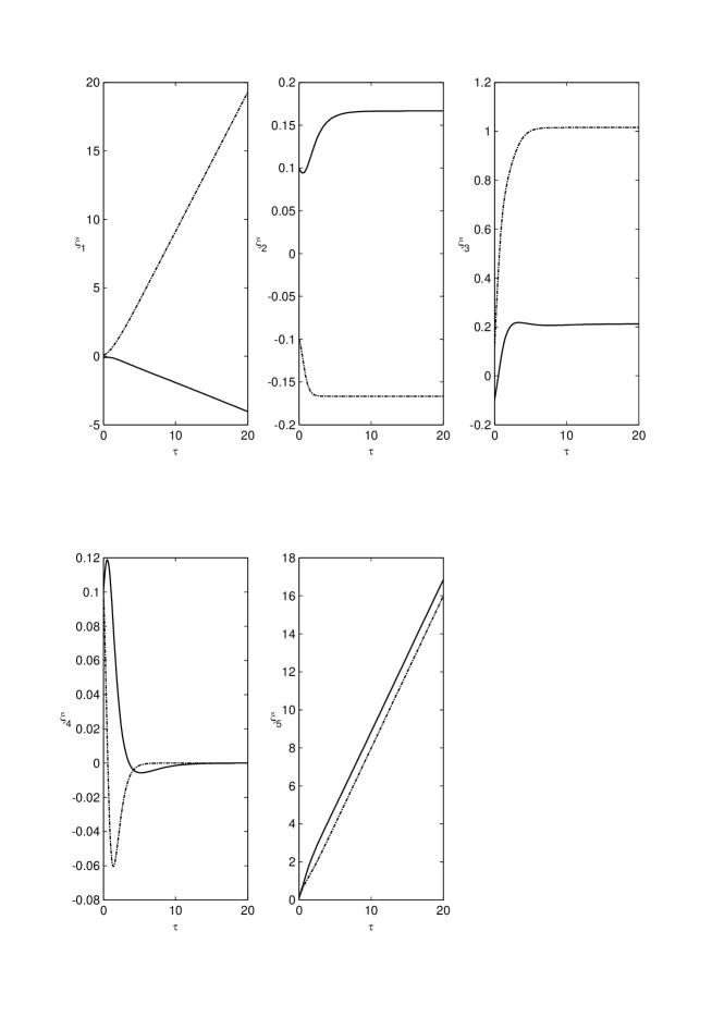
and for following relation$\frac{16(1-r)}{15r}<(V_{a}-V_{b})^{2}.$

Figure 2: r=$\frac{\rho_{a}}{\rho_{b}}=0.4$;Lower fluid denser.Dashed line for spike (heavier fluid pushes into lighter fluid) and unbroken line for bubble.$V_{a}=0.8,V_{b}=-0.6$.Initial condition as in Fig.1.

On the other hand if $r=\rho_{a}/\rho_{b}<1(A_{T}=\frac{\rho_{a}-\rho_{b}}{\rho_{a}+\rho_{b}}<0)$ there is no RT instability but it follows from Eqs.(37)and (38) that instability due to velocity shear (Kelvin -Helmholtz instability) persists on both the wind ward side and leeward side (i.e; both for bubbles and spikes) if (see Fig.2)

$$\frac{32|A_{T}|}{15(1+A_{T})}=\frac{16(1-r)}{15r}<(V_{a}-V_{b})^{2}$$ (39)

and stabilized on both sides if (see Fig.3 which shows oscillation of $\xi_{1}$and $\xi_{3}$ with respect to $\tau$)

$$(V_{a}-V_{b})^{2}<\frac{16}{15}(1-r)$$ (40)

If however $(V_{a}-V_{b})^{2}$ lies in the interval specified by the above inequalities,i.e;

$$\frac{16}{15}(1-r)<(V_{a}-V_{b})^{2}<\frac{16(1-r)}{15r};\mbox{(}r<1)$$ (41)

it follows from the same two Eqs.(37)-(38) that the peak of the spike continues to steeper (instability) with $\tau$ as the heavier fluid (density $\rho_{b}$)pushes across the interface into the lighter fluid (density $\rho_{a}$) while the bubble height will execute low finite amplitude undulations. The above observation is shown to be suppressed in Fig.4. At time t, the peak height which of the spike or the bubble occurs at $x=\eta_{1}(\tau)$ and thus moves to the right (x-increases) as $\eta_{1}(\tau)$ increases with $\tau$. The spike peak height increase monotonically with t while that of the bubble undulates with low amplitude. The three dimension representation of the steepening of the peak of the spike as it moves along x-direction with time is shown in Fig.5.In this respect there exists approximate qualitative agreement exists with the results of the weakly nonlinear analysis${}^{\cite[cite]{[\@@bibref{}{lw10}{}{}]}}$.

(B) Combined effect of Richtmyer-Meshkov and Kelvin-Helmholtz instability: oblique shock

The time evolution of the two fluid interfacial structure resulting from the combined effect of Richtmyer-Meshkov and Kelvin-Helmholtz instabilities consequent to impingement of an shock is described by the set of Eqs.(18)-(22),(26)-(29) with modifications as shown in the set of Eq.(31). If the shock incidence is oblique then the normal component generates velocity shear and causes KH instability.${}^{\cite[cite]{[\@@bibref{}{m94}{}{}]}}$ The shock generated initial values of $\overline{\xi}_{3}$ and $\overline{\xi}_{4}$ are obtained from the impulsive accelerations represented by the $\delta-$ function terms in Eq.(30) giving

$$(\overline{\xi}_{3})_{\tau=0}=\left[\frac{2(1-r)\xi_{2}(6\xi_{2}-1)}{D_{1}(\xi_{2},r)}\right]_{{(\xi_{2})}{\tau=0}}$$ (42)

$$(\overline{\xi}_{4})_{\tau=0}=\frac{1}{D_{2}(\xi_{2},r)}\left[\frac{(2\xi_{2}-1)(u_{b}-ru_{a})+2\xi_{2}(u_{a}-u_{b})}{\Delta v}\right]_{(\xi_{2})_{\tau=0}}$$ (43)

Results obtained from numerical solution of Eqs.(18)-(22) with modifications given by Eq.(31) subject to initial conditions (42) and (43) are presented in Fig.6. The growth rate contributed in absence of velocity shear,i.e; by normally incident shock induced Richtmyer-Meshkov instability varies as $t\rightarrow\infty$. However in presence of velocity shear the growth rate due to combined influence of RM and KH instability the growth rate approaches finite saturation value asymptotically.

For RM-KH instability induced spikes it is given by the following closed expression

$$(\overline{\xi}_{3})_{t\rightarrow\infty}^{spike}=(\frac{d\xi_{1}}{dt})_{t\rightarrow\infty}^{spike}=\sqrt{\frac{5(1+A_{T})}{16(1-A_{T})}(u_{a}-u_{b})^{2}/(\Delta v)^{2}}$$ (44)

which becomes large as the Atwood number $A_{T}\rightarrow$1 (equivalently$\rho_{a}/\rho_{b}>>1)$

The following discussions suggest a higher plausibility of the effectiveness of the joint influence of RM and KH instability in the explanation of certain astrophysical phenomena.

Corresponding to parameter values for Eagle Nebula($\rho_{a}/\rho_{b}=0.5\times 10^{2}$ and $|u_{a}-u_{b}|=2\times 10^{6}$ cm sec^-1)${}^{\cite[cite]{[\@@bibref{}{br06}{}{}]}},^{\cite[cite]{[\@@bibref{}{dd02}{}{}]}}$ the velocity of rise of the spike peak height h^spike(the height of the pillar) according to Eq.(44)is $(\frac{dh}{dt})_{t\rightarrow\infty}^{spike}\approx 0.79\times 10^{7}$cm sec^-1. Modification through inclusion of Rayleigh-Taylor instability effect (see Eq.(38)) can only slightly increases this value to $\approx 10^{7}$cm sec^-1.This gives the time to reach the observed pillar height of $3\times 10^{19}$ cm of the Eagle Nebula $\approx 10^{4}$ years. There are different time scales involved in the problem of development of the pillar of the Eagle Nebula. As pointed out by Pound, ${}^{\cite[cite]{[\@@bibref{}{mw98}{}{}]}}$ there is a characteristic time scale for hydrodynamic motion $\tau_{dyn}\approx(\Delta v)^{-1}$ where $\Delta v$ is the velocity shear inside the cloud. Corresponding to data given in ref.(3) this turns out to be $\tau_{hydrodanmic}\approx 10^{5}$yrs which is the upper time limit for development of the Eagle Nebula pillar(”elephant trunk”). But it is at least two orders of magnitude greater than the time scale $\tau_{cool}\sim 10^{2}-10^{3}$ yrs imposed due to radiative cooling of the cloud ${}^{\cite[cite]{[\@@bibref{}{br06}{}{}]}},^{\cite[cite]{[\@@bibref{}{dd02}{}{}]}}$. In comparison the time scale of the development of the pillar is found here $\approx 10^{4}$yrs. Thus consequent to the hydrodynamic model based on the combined influence of Richtmyer-Meshkov and Kelvin-Helmholtz instability the gap between the two time scales $\tau_{cool}$ and $\tau_{hydrodynamic}$is reduced by one order of magnitude.

A high Mach number, radiatevily cooled jet of astrophysical interest has been produced in laboratory using intense laser irradiation of a gold cone${}^{\cite[cite]{[\@@bibref{}{df99}{}{}]}}$. The evolution of the jet was imaged in emission and radiography.

K-H instability growth rate has recently been observed in HED plasma experiment using Omega laser ($\lambda$)=0.351$\mu m$ delivering 4.3 $\pm 0.1$kJ to the target overlapping 10 drive beams on to the ablator ${}^{\cite[cite]{[\@@bibref{}{eh09}{}{}]}}$.Incompressible K-H growth rate peak to valley at Foam-Plastic interface has been compared with several analytical modes.

V. Summary

Finally we summarize the results:

(a)If the heavier fluid overlies the lighter fluid the growth rate of both the bubble and spike peak heights due to RT instability are enhanced due to concurrent presence of velocity shear, i.e, K.H instability Fig.1. The asymptotic growth rates are given by Eqs. (37) and (38).

(b) In the opposite case,i.e, if the overlying fluid is lighter and lower one is heavier ($r=\rho_{a}/\rho_{b}<1$) both the spike and bubble peak displacement increases continuously with time if $\frac{16(1-r)}{15r}<(V_{a}-V_{b})^{2}$,i.e, instability persists (Fig.3) while stabilization occurs if $(V_{a}-V_{b})^{2}<\frac{(16(1-r)}{15})$ (Fig. 4 shows oscillation of peak heights of bubbles and spikes).

(c) For $\frac{16(1-r)}{15}<(V_{a}-V_{b})^{2}<\frac{16(1-r)}{15r}$ for r$<1$ the spike steepens with time (the peak height continuously increases with time as indicated in Fig.5. gives a three dimensional graph of displacement y against x and $\tau$). But the peak displacement of the bubble undulates within a small range Fig.4.

(d)If the two fluid interface is subjected to an oblique shock Kelvin-Helmholtz instability due to generation of velocity shear occurs simultaneously with Richtmyer-Meshkov instability.The growth rates of bubbles and spikes due to this joint action are shown in Fig.6. respectively. It is important to note that the growth rate of the combined action tends asymptotically to a saturation value given by Eq.(44); this is in contrast to that due to generation of RM instability due to normal shock incidence for which the growth rate behaves as $\frac{1}{t}$ as t$\rightarrow\infty$. Moreover this growth rate as shown by Eq.(44) the rate of growth of this spike height has sufficiently large magnitude if the Atwood number $A_{T}\rightarrow$1($\rho_{a}<<\rho_{b}$).This may have interesting implication in the hydrodynamic explanation of formation of sufficiently long spiky jets in astrophysical situation, e.g, in case of the Eagle Nebula.

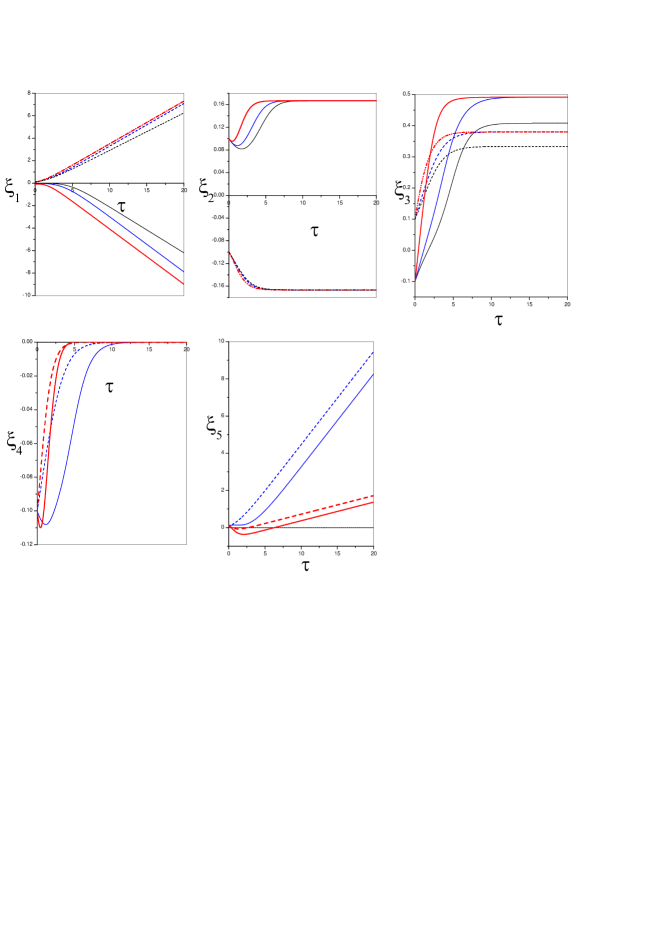
Figure 1: Initial values $r=\frac{\rho_{a}}{\rho_{b}}=1.5,\xi_{1}=-\xi_{2}=\xi_{3}=\xi_{4}=\xi_{5}=0.1$ for bubble;$-\xi_{1}=\xi_{2}=-\xi_{3}=\xi_{4}=\xi_{5}=0.1$ for spike.Plot showing variation of $\xi_{1},\xi_{2}$,growth rate $\xi_{3},\xi_{4}$ and transverse displacement $\xi_{5}$ of bubble and spike with $V_{a}=V_{b}=0.0$ for solid black line-spike and broken black line for bubble.$V_{a}=0.1,V_{b}=0.5$ for broken blue line-bubble and solid blue for spike,$V_{a}=0.5,V_{b}=0.1$,broken red line for bubble and solid red line-spike.

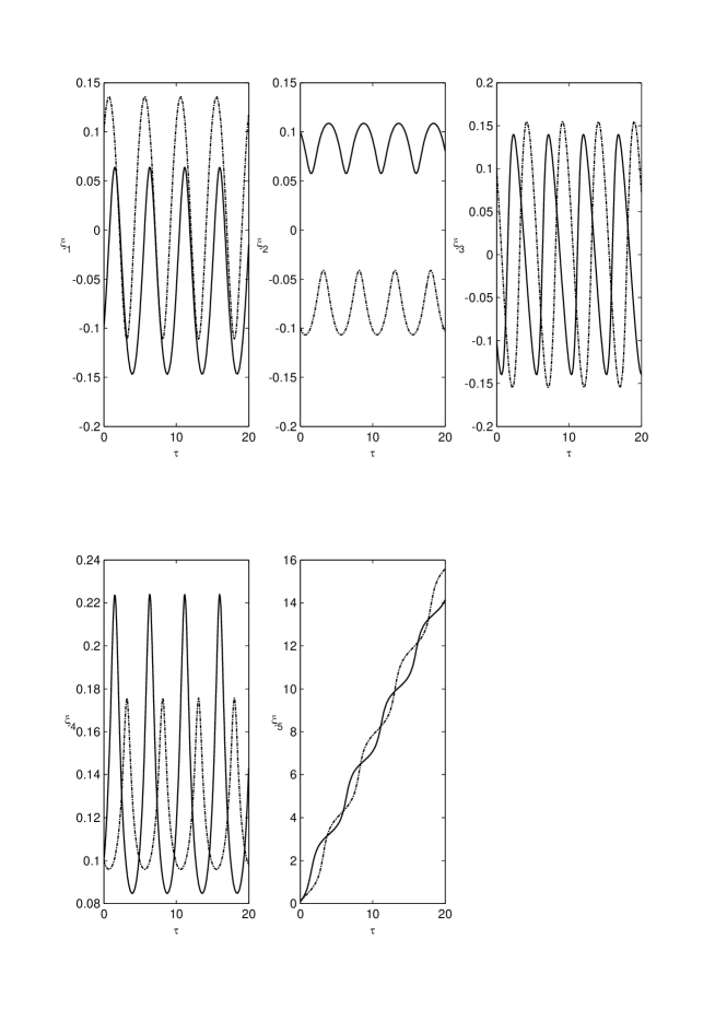
Figure 3: r=0.4,$V_{a}=0.0,V_{b}=0.2.(V_{a}-V_{b})^{2}<\frac{16(1-r)}{15}$ .Initial condition as in Fig.1. Unbroken line for bubble and dashed line for spike.

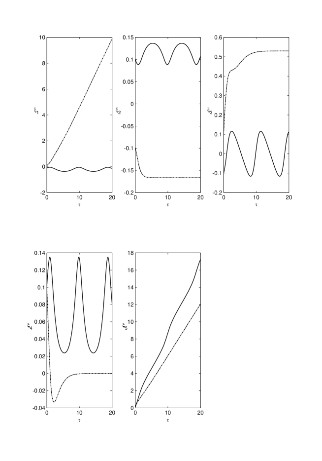
Figure 4: r=0.4,$V_{a}=0.6,V_{b}=-0.4;\frac{16(1-r)}{15}<(V_{a}-V_{b})^{2}<\frac{16(1-r)}{15r}$.Initial condition as before (Fig.3.).Unbroken line for bubble and dashed line for spike;height of spike peak increases monotonically with time (steepening);bubble depth undulates.

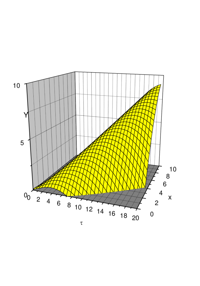
Figure 5: 3 dimensional plot of spike(Interface $Y=\eta_{0}(\tau)+\eta_{2}(\tau)(x-\eta_{1}(\tau))^{2}$)belonging to the plot given in fig.4.

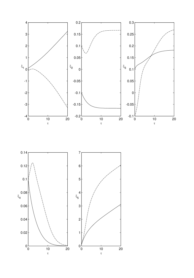
Figure 6: Oblique shock: RM and KH instability for spike (dashed line) and bubble (unbroken line).Initial values as in fig.1. and $V_{a}=0.1,V_{b}=0.5.$

References

• [1] R.P.Drake, High Energy Density Physics, Spinger, (2006).
• [2] K.Kifonidis,T.Plewa,H.T.Janka,E.Muller, Astron. and Astrophys. 408,621 (2003).
• [3] B.A.Remington,R.P.Drake and D.D.Ryutov, Rev. Mod. Phys. 78, 755 (2006).
• [4] D.D.Ryutov and B.A Remington, Plasma Phys. Control Fusion 44, B407 (2002).
• [5] B.A. Remington,R.P.Drake,H.Takabe and D.Arnett, Phys. Plasmas 7, 1641 (2000).
• [6] L.Spitzer,Jr., Astrophys. J. 120, 1 (1954).
• [7] E.A.Frieman, Astrophys. J. 120, 18 (1954).
• [8] T.Buhrke,R.Mundt and T.P.Ray Astron. and Astrophys. 200,99 (1988).
• [9] K.O.Mikaelian, Phys. Fluids 6, 1943 (1994).
• [10] L.F.Wang,W.H.Ye,Z.F.Fan,Y.J.Li,X.T.He and M.Y.Yu, Europhys. Lett. 86, 15002 (2009).
• [11] L.F.Wang,W.H.Ye,Y.J.Li, Europhys. Lett. 87,54005 (2009).
• [12] L.F.Wang,C.Xue,W.H.Ye and Y.J.Li, Phys. Plasmas 16, 112104 (2009).
• [13] L.F.Wang,W.H.Ye and Y.J.Li, Phys. Plasmas 17,052305 (2010).
• [14] J.Hecht, U.Alon and D.Shvarts, Phys. Fluids 6,4019 (1994).
• [15] A.L.Velikovich and G.Dimonte, Phys.Rev.Lett.76,3112 (1996).
• [16] G.Hazak, Phys.Rev.Lett. 76,4167 (1996).
• [17] Q.Zhang, Phys.Rev.Lett. 81,3391 (1998).
• [18] V.N.Goncharov, Phys.Rev.Lett. 88,134502 (2002).
• [19] S.I.Sohn, Phys.Rev. E 67,026301 (2003).
• [20] M.R.Gupta,S.Roy,M.Khan,H.C.Pant,S.Sarkar and M.K.Srivastava, Phys.Plasma. 16,032303 (2009).
• [21] D.Layzer, Astrophys. J. 122,1 (1955).
• [22] S.Chandrasekhar, Hydrodynamics and Hydrodynamic Stability, Dover,New York 1981.
• [23] M.R.Gupta,L.K.Mandal,S.Roy and M.Khan, Phys.Plasma. 17,012306 (2010).
• [24] M.W.Pound, Astrophys. J. 493,L113 (1998).
• [25] D.R.Farely,K.G.Estabrook,S.G.Glendinning,S.H.Glenzer,B.A.Remington,K.Shigemori,
J.M.Stone,R.J.Wallace,G.B.Zimmerman and J.A.Harte, Phy.Rev.Lett. 83, 1982 (1999).
• [26] E.C.Harding,J.F.Hansen,O.A.Hurricane,R.P.Drake,H.F.Robey,C.C.Kuranz,B.A.Remington,
M.J.Bono,M.J.Grosskopf and R.S.Gillespie, Phy.Rev.Lett. 103, 045005 (2009).
Refer to caption