Fourth generation effect on $\Lambda_{b}$ decays

Abstract

The rare decays of $\Lambda_{b}$ baryon governed by the quark level transitions $b\to s$, are investigated in the fourth quark generation model popularly known as SM4. Recently it has been shown that SM4, which is a very simple extension of the standard model, can successfully explain several anomalies observed in the CP violation parameters of $B$ and $B_{s}$ mesons. We find that in this model due to the additional contributions coming from the heavy $t^{\prime}$ quark in the loop, the branching ratios and other observables in rare $\Lambda_{b}$ decays deviate significantly from their SM values. Some of these modes are within the reach of LHCb experiment and search for such channels are strongly argued.

I Introduction

The rare decays of $B$ mesons involving flavor changing neutral current (FCNC) transitions are of great interest to look for possible hints of new physics beyond the standard model (SM). In the SM, the FCNC transitions arise only at one-loop level, thus providing an excellent testing ground to look for new physics. Therefore, it is very important to study FCNC processes, both theoretically and experimentally, as these decays can provide a sensitive test for the investigation of the gauge structure of the SM at the loop level. Huge experimental data on both exclusive and inclusive $B$ meson decays hfag involving $b\to s$ transitions have been accumulated at the $e^{+}e^{-}$ asymmetric $B$ factories operating at $\Upsilon(4S)$, which motivated extensive theoretical studies on these mesonic decay modes.

Unlike the mesonic decays, the experimental results on FCNC mediated $\Lambda_{b}$ baryon decays e.g., $\Lambda_{b}\to\Lambda\pi$, $\Lambda_{b}\to pK^{-}$, $\Lambda_{b}\to\Lambda\gamma$ and $\Lambda_{b}\to\Lambda l^{+}l^{-}$ are rather limited. At present we have only upper limits on some of these decay modes pdg . Heavy baryons containing a heavy $b$ quark will be copiously produced at the LHC. Their weak decays may provide important clues on flavor changing currents beyond the SM in a complementary fashion to the $B$ decays. A particular advantage of the bottom baryon decays over the $B$ mesons is that these decays are self-tagging processes which should make their experimental reconstructions easier.

Another important aspect is that, in the past few years we have seen some kind of deviations from the SM results in the CP violating observables of $B$ and $B_{s}$ meson decays involving $b\to s$ transitions hfag ; utfit ; browder ; soni10 ; lenz10 . Several new physics scenarios are proposed in literature to account for these deviations np . Therefore, it is quite natural to expect that if there is some new physics present in the $b\to s$ transitions of $B$ meson decays it must also affect the corresponding $\Lambda_{b}$ transitions. Therefore, the study of the rare $\Lambda_{b}$ decays is of utmost importance to obtain an unambiguous signal of new physics.

In this paper we would like to study the rare $\Lambda_{b}$ decays in a model with an extra generation of quarks, usually known as SM4 4gen . SM4 is a simple extension of the standard model with three generations (SM3) with the additional up-type ($t^{\prime}$) and down-type ($d^{\prime}$) quarks. The model retains all the properties of SM3. The $t^{\prime}$ quark like the other up-type quarks contribute to the $b\to s$ transition at the loop level. Due to the additional fourth generation there will be mixing between the $b^{\prime}$ quark the three down-type quarks of the standard model and the resulting mixing matrix will become a $4\times 4$ matrix ($V_{CKM4})$. The parametrization of this unitary matrix requires six mixing angles and three phases. The existence of the two extra phases provides the possibilities of extra source of CP violation. Another advantage of this model is that the heavier quarks and leptons in this family can play a crucial role in dynamical electroweak symmetry breaking as an economical way to address the hierarchy problem ewsb . The effect of fourth generation of quarks in various $B$ decays are extensively studied in the literature 4thgen . In Refs. rm1 ; buras , it has been shown that this model can easily explain the observed anomalies in the $B$ meson sector.

The paper is organized as follows. In section II we discuss the nonleptonic decay of $\Lambda_{b}$ baryon. The radiative decay process $\Lambda_{b}\to\Lambda\gamma$ is discussed in section III. The results on semileptonic decays are presented in section IV. Section V contains the summary and conclusion

II Decay width of $\Lambda_{b}\to\Lambda\pi^{0}$ and $\Lambda_{b}\to pK^{-}$ modes

In this section we will discuss the nonleptonic rare $\Lambda_{b}$ decay mode $\Lambda_{b}\to\Lambda\pi$ and $\Lambda_{b}\to pK^{-}$ induced by the quark level transition $b\to sq\bar{q},~{}(q=u,d)$. The effective Hamiltonian describing these processes is given by hycheng

$${\cal H}_{eff}=\frac{G_{F}}{\sqrt{2}}\left[V_{ub}V_{us}^{*}\sum_{i=1,2}C_{i}(\mu)O_{i}-V_{tb}V_{ts}^{*}\sum_{i=3}^{10}C_{i}(\mu)O_{i}\right],$$ (1)

where $C_{i}(\mu)$’s are the Wilson coefficients evaluated at the renormalization scale $\mu$, $O_{1,2}$ are the tree level current-current operators, $O_{3-6}$ are the QCD and $O_{7-10}$ are electroweak penguin operators.

Let us first consider the decay process $\Lambda_{b}\to\Lambda\pi$. In the SM this mode receives contributions from the color-suppressed tree and the electroweak penguin diagrams and the amplitude for this process in the factorization approximation is given as rm2001

$${\cal A}(\Lambda_{b}(p)\to\Lambda(p^{\prime})\pi^{0}(q)) = \frac{G_{F}}{\sqrt{2}}\Big{[}V_{ub}V_{us}^{*}a_{2}-V_{tb}V_{ts}^{*}\left(\frac{3}{2}(a_{9}-a_{7})\right)\Big{]}$$ (2)

$$\times \langle\Lambda(p^{\prime})|(\bar{s}\gamma^{\mu}(1-\gamma_{5})b|\Lambda_{b}(p)\rangle\langle\pi^{0}(q)|\bar{u}\gamma_{\mu}(1-\gamma_{5})u|0\rangle,$$

where $a_{i}=C_{i}+C_{i+1}/N~{}(C_{i}+C_{i-1}/N)$ for $i$= odd (even). In order to evaluate the matrix elements we use the following form factors and decay constants. The matrix elements of the various hadronic currents between initial $\Lambda_{b}$ and the final $\Lambda$ baryon, are parameterized in terms of various form factors cdlu as

$$\langle\Lambda(p^{\prime})|\bar{s}\gamma_{\mu}b|\Lambda_{b}(p)\rangle = \bar{u}_{\Lambda}(p^{\prime})\Big{[}g_{1}(q^{2})\gamma_{\mu}+ig_{2}(q^{2})\sigma_{\mu\nu}q^{\nu}+g_{3}(q^{2})q_{\mu}\Big{]}u_{\Lambda_{b}}(p)\;,$$

$$\langle\Lambda(p^{\prime})|\bar{s}\gamma_{\mu}\gamma_{5}b|\Lambda_{b}(p)\rangle = \bar{u}_{\Lambda}(p^{\prime})\Big{[}G_{1}(q^{2})\gamma_{\mu}+iG_{2}(q^{2})\sigma_{\mu\nu}q^{\nu}+G_{3}(q^{2})q_{\mu}\Big{]}\gamma_{5}u_{\Lambda_{b}}(p)\;,$$ (3)

where $g_{i}~{}(G_{i})$’s are the vector (axial vector) form factors and $q$ is the momentum transfer i.e., $q=p-p^{\prime}$. The matrix element $\langle\pi(q)|\bar{u}\gamma_{\mu}\gamma_{5}u|0\rangle$ is related to the pion decay constant $f_{\pi}$ as

$$\langle\pi^{0}(q)|\bar{u}\gamma^{\mu}\gamma_{5}u|0\rangle=if_{\pi}q^{\mu}/\sqrt{2}.$$ (4)

With these values one can write the transition amplitude for $\Lambda_{b}\to\Lambda\pi$ as

$${\cal A}(\Lambda_{b}\to\Lambda\pi^{0}) = i\frac{G_{F}}{2}f_{\pi}\left(V_{ub}V_{us}^{*}a_{2}-\frac{3}{2}V_{tb}V_{ts}^{*}(a_{9}-a_{7})\right)$$ (5)

$$\times \bar{u}_{\Lambda}(p^{\prime})\biggr{[}\Big{(}g_{1}(q^{2})(m_{\Lambda_{b}}-m_{\Lambda})+g_{3}(q^{2})m_{\pi}^{2}\Big{)}$$

$$+ \Big{(}G_{1}(q^{2})(m_{\Lambda_{b}}+m_{\Lambda})-G_{3}(q^{2})m_{\pi}^{2}\Big{)}\gamma_{5}\biggr{]}u_{\Lambda_{b}}(p).$$

The above amplitude can be symbolically written as

$${\cal A}(\Lambda_{b}(p^{\prime})\to\Lambda(p)\pi^{0}(q))=i\bar{u}_{\Lambda}(p^{\prime})(A+B\gamma_{5})u_{\Lambda_{b}}(p)\;,$$ (6)

where $A$ and $B$ are given as

$$A = \frac{G_{F}}{2}f_{\pi}\left(V_{ub}V_{us}^{*}a_{2}-\frac{3}{2}V_{tb}V_{ts}^{*}(a_{9}-a_{7})\right)\times\Big{(}g_{1}(q^{2})(m_{\Lambda_{b}}-m_{\Lambda})+g_{3}(q^{2})m_{\pi}^{2}\Big{)},$$

$$B = \frac{G_{F}}{2}f_{\pi}\left(V_{ub}V_{us}^{*}a_{2}-\frac{3}{2}V_{tb}V_{ts}^{*}(a_{9}-a_{7})\right)\times\Big{(}G_{1}(q^{2})(m_{\Lambda_{b}}+m_{\Lambda})-G_{3}(q^{2})m_{\pi}^{2}\Big{)}.$$ (7)

Thus, one can obtain the decay width for this process as pakvasa ,

$$\Gamma=\frac{p_{cm}}{8\pi}\left[\frac{(m_{\Lambda_{b}}+m_{\Lambda})^{2}-m_{\pi}^{2}}{m_{\Lambda_{b}}^{2}}|A|^{2}+\frac{(m_{\Lambda_{b}}-m_{\Lambda})^{2}-m_{\pi}^{2}}{m_{\Lambda_{b}}^{2}}|B|^{2}\right],$$ (8)

where $p_{cm}$ is magnitude of the center-of-mass momentum of the outgoing particles.

For numerical analysis we use the following input parameters. The masses of the particles, the decay constant of pion and the lifetime of $\Lambda_{b}$ baryon are taken from pdg . The values of the effective Wilson coefficients are taken from rm2001 . The values of the CKM elements used are $|V_{ub}|=(3.93\pm 0.36)\times 10^{-3}$, $|V_{us}|=(0.2255\pm 0.0019)$, $|V_{tb}|=0.999$, $|V_{ts}|=(38.7\pm 2.3)\times 10^{-3}$ pdg and the weak phase $\gamma=\left(70_{-21}^{+14}\right)^{\circ}$ ckmfitter .

To evaluate the branching ratio for $\Lambda_{b}\to\Lambda\pi$ decay we need to specify the form factors describing $\Lambda_{b}\to\Lambda$ transition. In this analysis we use the values of the factors from cdlu which are evaluated using the light-cone sum rules. In this approach, the dependence of form factors on the momentum transfer can be parameterized as

$$\xi_{i}(q^{2})=\frac{\xi_{i}(0)}{1-a_{1}(q^{2}/m_{\Lambda_{b}}^{2})+a_{2}(q^{4}/m_{\Lambda_{b}}^{4})}\;,$$ (9)

where $\xi$ denotes the form factor $g_{1}$ and $g_{2}$. The values of the parameters $\xi_{i}(0)$, $a_{1}$ and $a_{2}$ have been presented in Table-1. The other form factors can be related to these two as

$$g_{1}=G_{1},~{}~{}~{}~{}~{}g_{2}=G_{2}=g_{3}=G_{3}.$$ (10)

Table 1: Numerical values of the form factors $g_{1}$ and $g_{2}$ and the parameters $a_{1}$ and $a_{2}$ involved in the double fit (9).

parameter		twist-3		up to twist-6
$g_{1}(0)$		$0.14_{-0.01}^{+0.02}$		$0.15_{-0.02}^{+0.02}$
$a_{1}$		$2.91_{-0.07}^{+0.10}$		$2.94_{-0.06}^{+0.11}$
$a_{2}$		$2.26_{-0.08}^{+0.13}$		$2.31_{-0.10}^{+0.14}$
$g_{2}(0)(10^{-2}~{}{\rm GeV^{-1}})$		$-0.47_{-0.06}^{+0.06}$		$1.3_{-0.4}^{+0.2}$
$a_{1}$		$3.40_{-0.05}^{+0.06}$		$2.91_{-0.09}^{+0.12}$
$a_{2}$		$2.98_{-0.08}^{+0.09}$		$2.24_{-0.13}^{+0.17}$

Thus, we obtain the branching ratio for $\Lambda_{b}\to\Lambda\pi$ mode in the SM as

$${\rm Br}(\Lambda_{b}\to\Lambda\pi) = (6.4\pm 2.0)\times 10^{-8}~{}~{}~{}~{}(\rm twist-3)$$

$${\rm Br}(\Lambda_{b}\to\Lambda\pi) = (7.4\pm 2.3)\times 10^{-8}~{}~{}~{}~{}(\rm up~{}to~{}twist-6),$$ (11)

where we have assumed $50\%$ uncertainties due to non-factorizable contributions. It should be noted that these values are beyond the reach of the currently running experiments and hence, observation of this mode will be a clear signal of new physics.

In the presence of a fourth generation of quarks, there will be additional contribution due to the $t^{\prime}$ quark in the electroweak penguin loops. Furthermore, it should be noted that due to the presence of $t^{\prime}$ quark the unitarity condition becomes $\lambda_{u}+\lambda_{c}+\lambda_{t}+\lambda_{t^{\prime}}=0$, where $\lambda_{q}=V_{qb}V_{qs}^{*}$.

Thus, in the presence of the fourth generation of quarks the amplitude for $\Lambda_{b}\to\Lambda\pi$ will become

$${\cal A}(\Lambda_{b}\to\Lambda\pi^{0})=i\left(\lambda_{u}a_{2}-\frac{3}{2}\lambda_{t}(a_{9}-a_{7})-\frac{3}{2}\lambda_{t^{\prime}}(a^{\prime}_{9}-a^{\prime}_{7})\right)\times\bar{u}_{\Lambda}(p^{\prime})(X+Y\gamma_{5})u_{\Lambda_{b}}(p),$$ (12)

where $X$ and $Y$ are given as

$$X = \frac{G_{F}}{2}f_{\pi}\Big{(}g_{1}(q^{2})(m_{\Lambda_{b}}-m_{\Lambda})+g_{3}(q^{2})m_{\pi}^{2}\Big{)},$$

$$Y = \frac{G_{F}}{2}f_{\pi}\Big{(}G_{1}(q^{2})(m_{\Lambda_{b}}+m_{\Lambda})-G_{3}(q^{2})m_{\pi}^{2}\Big{)}.$$ (13)

The above amplitude can be represented in a more general way

$${\cal A}(\Lambda_{b}(p^{\prime}) \to \Lambda(p)\pi^{0}(q))=i[\bar{u}_{\Lambda}(X+Y\gamma_{5})u_{\Lambda_{b}}]$$ (14)

$$\times \lambda_{u}a_{2}\Big{(}1+ra\exp(i(\delta+\gamma)-br^{\prime}\exp(i(\delta^{\prime}+\phi_{s}+\gamma))\Big{)},$$

where the parameters $a$, $b$, $r$, $r^{\prime}$ and the strong phases $\delta$ and $\delta^{\prime}$ are defined as

$$a = |\lambda_{t}/\lambda_{u}|,~{}~{}~{}~{}b=|\lambda_{t}^{\prime}/\lambda_{u}|,~{}~{}~{}~{}r=\frac{3}{2}\left|\frac{a_{9}-a_{7}}{a_{2}}\right|,~{}~{}~{}~{}~{}~{}~{}r^{\prime}=\frac{3}{2}\left|\frac{a_{9}^{\prime}-a_{7}^{\prime}}{a_{2}}\right|$$

$$\delta = \arg\left(\frac{a_{9}-a_{7}}{a_{2}}\right),~{}~{}~{}\delta^{\prime}=\arg\left(\frac{a_{9}^{\prime}-a_{7}^{\prime}}{a_{2}}\right).$$ (15)

The weak phases of the CKM elements are used as : $(-\gamma)$ the phase of $V_{ub}$, $\pi$ is the phase of $V_{ts}$ and $\phi_{s}$ is the phase of $\lambda_{t^{\prime}}$. The decay width for this process can be given by

$$\Gamma = \frac{p_{cm}}{8\pi}|\lambda_{u}a_{2}|^{2}\left[\frac{(m_{\Lambda_{b}}+m_{\Lambda})^{2}-m_{\pi}^{2}}{m_{\Lambda_{b}}^{2}}|X|^{2}+\frac{(m_{\Lambda_{b}}-m_{\Lambda})^{2}-m_{\pi}^{2}}{m_{\Lambda}^{2}}|Y|^{2}\right]$$

$$\times \Big{[}1+a^{2}r^{2}+b^{2}r^{\prime 2}+2ar\cos(\delta+\gamma)-2br^{\prime}\cos(\phi_{s}+\gamma+\delta^{\prime})-2abrr^{\prime}\cos(\phi_{s}+\delta^{\prime}-\delta)\Big{]}.$$

For numerical evaluation of the branching ratio we need to know the values of the new parameters of this model. We use the allowed range for the new CKM elements as $|\lambda_{t^{\prime}}|=(0.08\rightarrow 1.4)\times 10^{-2}$ and $\phi_{s}=(0\rightarrow 80)^{\circ}$ for $m_{t^{\prime}}=400$ GeV, extracted using the available observables which are mediated through $b\to s$ transitions rm1 . To find out the values of the QCD parameters $a_{9}^{\prime}$ and $a_{7}^{\prime}$ we need to evaluate the new Wilson coefficients $C_{7-10}^{\prime}$ due to the virtual $t^{\prime}$ quark exchange in the loop. The values of these coefficients at $M_{W}$ scale can be obtained from the corresponding contribution due to $t$-quark exchange by replacing the mass of $t$ quark in the Inami-Lim functions inami by $m_{t^{\prime}}$. These values can then be evolved to the $m_{b}$ scale using the renormalization group equation as discussed in buras1 . The values of these coefficients for a representative $t^{\prime}$ mass mass $m_{t^{\prime}}=400$ GeV listed in Table-2.

Table 2: Numerical values of the Wilson coefficients $C_{i}^{\prime}$ for $m_{t^{\prime}}=400$ GeV.

$C_{3}^{\prime}$	$C_{4}^{\prime}$	$C_{5}^{\prime}$	$C_{6}^{\prime}$
$2.06\times 10^{-2}$	$-3.85\times 10^{-2}$	$1.02\times 10^{-2}$	$-4.43\times 10^{-2}$
$C_{7}^{\prime}$	$C_{8}^{\prime}$	$C_{9}^{\prime}$	$C_{10}^{\prime}$
$4.453\times 10^{-3}$	$2.115\times 10^{-3}$	$-0.029$	$0.006$

With these inputs the variation of the branching ratio for the $\Lambda_{b}\to\Lambda\pi$ with $|\lambda_{t}^{\prime}|$ is shown in Figure-1. From the figure it can be seen that the branching ratio is significantly enhanced from its corresponding SM value and it could be easily accessible in the currently running LHCb experiment.

Figure 1: The branching ratio versus $|\lambda_{t}^{\prime}|$ for the process $\Lambda_{b}\to\Lambda\pi$.

Now we will discuss the decay mode $\Lambda_{b}$ decay mode $\Lambda_{b}\to pK^{-}$, mediated through $b\to s$ transition. In the SM, it receives contributions from color allowed tree, QCD as well as electroweak penguins. Its amplitude in the SM is given as rm2001

$${\cal A}(\Lambda_{b}\to pK^{-}) = i\frac{G_{F}}{\sqrt{2}}f_{K}\bar{u}_{p}(p^{\prime})\Big{[}\Big{(}\lambda_{u}a_{1}-\lambda_{t}(a_{4}+a_{10}+(a_{6}+a_{8})R_{1}\Big{)}$$ (17)

$$\times (g_{1}(m_{K}^{2})(m_{\Lambda_{b}}-m_{\Lambda})+g_{3}(m_{K}^{2})m_{K}^{2})$$

$$+ \Big{(}\lambda_{u}a_{1}-\lambda_{t}(a_{4}+a_{10}-(a_{6}+a_{8})R_{2}\Big{)}$$

$$\times \Big{(}G_{1}(m_{K}^{2})(m_{\Lambda_{b}}+m_{\Lambda})-G_{3}(m_{K}^{2})m_{K}^{2}\Big{)}\gamma_{5}\Big{]}u_{\Lambda_{b}}(p),$$

where

$$R_{1}=\frac{2m_{K}^{2}}{(m_{b}-m_{u})(m_{s}+m_{u})},~{}~{}~{}~{}~{}~{}~{}R_{2}=\frac{2m_{K}^{2}}{(m_{b}+m_{u})(m_{s}+m_{u})}.$$ (18)

From the above amplitude one can obtain the branching ratio using Eq. (8). Using the input parameters as discussed earlier in this section and assuming $50\%$ uncertainties due to nonfactorizable contributions, we obtain the branching ratio in the SM

$${\rm Br}(\Lambda_{b}\to pK^{-})=3.5\times 10^{-6}$$ (19)

which is lower than the present experimental value ${\rm Br}(\Lambda_{b}\to pK^{-})=(5.6\pm 0.8\pm 1.5)\times 10^{-6}$ alto . Here we have used the form factors for $\Lambda_{b}\to p$ transitions from ztwei , which are evaluated in the light-front quark model. The $q^{2}$ dependence of the form factors are given by the following three parameters fit as

$$\xi_{i}(q^{2})=\frac{\xi_{i}(0)}{(1-q^{2}/m_{\Lambda_{b}}^{2})(1-a_{1}(q^{2}/m_{\Lambda_{b}}^{2})+a_{2}(q^{4}/m_{\Lambda_{b}}^{4})}\;,$$ (20)

where the values of the different fit parameters are listed in Table-3.

Table 3: Numerical values of the form factors $g_{1}$ and $g_{2}$ and the parameters $a_{1}$ and $a_{2}$ for $\Lambda_{b}\to p$ transition (20).

$\xi$		$\xi(0)$		$a$		$b$
$g_{1}$		$0.1131$		1.70		1.60
$g_{3}$		$0.0356$		2.5		2.57
$G_{1}$		$0.1112$		1.65		1.60
$G_{3}$		$0.0097$		2.8		2.7

As discussed earlier in the presence of a fourth generation of quarks the amplitude (17) will receive additional contributions due to the heavy $t^{\prime}$ quark in the loop. The modified amplitude becomes

$${\cal A}(\Lambda_{b}\to pK^{-}) = i\frac{G_{F}}{\sqrt{2}}f_{K}\bar{u}_{p}\Big{[}\Big{(}\lambda_{u}a_{1}-\lambda_{t}(a_{4}+a_{10}+(a_{6}+a_{8})R_{1})$$ (21)

$$- \lambda_{t^{\prime}}(a_{4}^{\prime}+a_{10}^{\prime}+(a_{6}^{\prime}+a_{8}^{\prime})R_{1})\Big{)}(g_{1}(m_{K}^{2})(m_{\Lambda_{b}}-m_{\Lambda})+g_{3}(m_{K}^{2})m_{K}^{2})$$

$$+ \Big{(}\lambda_{u}a_{1}-\lambda_{t}(a_{4}+a_{10}-(a_{6}+a_{8})R_{2}-\lambda_{t^{\prime}}(a_{4}^{\prime}+a_{10}^{\prime}-(a_{6}^{\prime}+a_{8}^{\prime})R_{2})\Big{)}$$

$$\times \Big{(}G_{1}(m_{K}^{2})(m_{\Lambda_{b}}+m_{\Lambda})-G_{3}(m_{K}^{2})m_{K}^{2}\Big{)}\gamma_{5}\Big{]}u_{\Lambda_{b}}.$$

Now using the values of the new Wilson coefficients $C_{3-10}^{\prime}$ from Table-2 and varying the new CKM elements between $0.0008\leq|\lambda_{t^{\prime}}|\leq 0.014$ and $(0\leq\phi_{s}\leq 80)^{\circ}$, we present in Figure-2 the variation of Br($\Lambda_{b}\to pK^{-})$ with $|\lambda_{t^{\prime}}|$. From the figure it can be seen that the measured branching ratio can be easily accommodated in this model.

Figure 2: The branching ratio versus $|\lambda_{t}^{\prime}|$ for the process $\Lambda_{b}\to pK^{-}$, where the horizontal line represents the experimental central value.

III $\Lambda_{b}\to\Lambda\gamma$ decay width

In this section we will consider the rare radiative decay $\Lambda_{b}\to\Lambda\gamma$ which is induced by the quark level transition $b\to s\gamma$. The effective Hamiltonian describing $\Lambda_{b}\to\Lambda\gamma$ is given as

$${\cal H}_{eff}=-\frac{4G_{F}}{\sqrt{2}}\lambda_{t}C_{7}(m_{b})O_{7},$$ (22)

where $C_{7}$ is the Wilson coefficient and $O_{7}$ is the electromagnetic dipole operator given as

$$O_{7}=\frac{e}{32\pi^{2}}F_{\mu\nu}[m_{b}\bar{s}\sigma^{\mu\nu}(1+\gamma_{5})b+m_{s}\bar{s}\sigma^{\mu\nu}(1-\gamma_{5})b]$$ (23)

The expression for calculating the Wilson coefficient $C_{7}(\mu)$ is given in buras2 . The matrix elements of the various hadronic currents between initial $\Lambda_{b}$ and the final $\Lambda$ baryon, which are parameterized in terms of various form factors as

$$\langle\Lambda|\bar{s}i\sigma_{\mu\nu}q^{\nu}b|\Lambda_{b}\rangle = \bar{u}_{\Lambda}\Big{[}f_{1}\gamma_{\mu}+if_{2}\sigma_{\mu\nu}q^{\nu}+f_{3}q_{\mu}\Big{]}u_{\Lambda_{b}}\;,$$

$$\langle\Lambda|\bar{s}i\sigma_{\mu\nu}\gamma_{5}q^{\nu}b|\Lambda_{b}\rangle = \bar{u}_{\Lambda}\Big{[}F_{1}\gamma_{\mu}\gamma_{5}+iF_{2}\sigma_{\mu\nu}\gamma_{5}q^{\nu}+F_{3}\gamma_{5}q_{\mu}\Big{]}u_{\Lambda_{b}}\;,$$ (24)

These form factors are related to the previously defined $g_{1}$ and $g_{2}$ through cdlu

$$F_{1}(q^{2})=f_{1}(q^{2})=q^{2}g_{2}(q^{2})=q^{2}G_{2}(q^{2}),$$

$$F_{2}(q^{2})=f_{2}(q^{2})=g_{1}(q^{2})=G_{1}(q^{2}).$$ (25)

Thus, one can obtain the decay width of $\Lambda_{b}\to\Lambda\gamma$ in the SM as

$$\Gamma(\Lambda_{b}\to\Lambda\gamma)=\frac{\alpha G_{F}^{2}}{32m_{\Lambda_{b}}^{3}\pi^{4}}|V_{tb}V_{ts}^{*}|^{2}|C_{7}|^{2}(1-x^{2})^{3}(m_{b}^{2}+m_{s}^{2})[f_{2}(0)]^{2},$$ (26)

where $x=m_{\Lambda}/m_{\Lambda_{b}}$. Using the input parameters as discussed in section II we obtain the branching ratio in the SM as

$${\rm Br}(\Lambda_{b}\to\Lambda\gamma)=(7.93\pm 2.31)\times 10^{-6},$$ (27)

which is well below the present experimental upper limit ${\rm Br}(\Lambda_{b}\to\Lambda\gamma)<1.3\times 10^{-3}$ pdg . Now we would like to see the effect of fourth quark generation on the branching ratio of $\Lambda_{b}\to\Lambda\gamma$. In the presence of fourth quark generation of quarks, the Wilson coefficient $C_{7}$ will be modified due to the $t^{\prime}$ contribution in the loop. Thus the modified parameter can be given as

$$C_{7}^{\rm tot}(\mu)=C_{7}(\mu)+\frac{V_{t^{\prime}b}V_{t^{\prime}s}^{*}}{V_{tb}V_{ts}^{*}}C_{7}^{\prime}(\mu).$$ (28)

where $C_{7}^{\prime}$ can be obtained from the expression of $C_{7}$ by replacing the mass of $t$ quark by $m_{t^{\prime}}$. The value of $C_{7}^{\prime}$ for $m_{t^{\prime}}=400$ GeV is found to be $C_{7}^{\prime}=-0.375$.

Thus, in SM4 the branching ratio can be given by Eq. (26) by replacing $C_{7}$ by $C_{7}^{tot}$. Now varying $\lambda_{t^{\prime}}$ between $0.0008\leq|\lambda_{t}^{\prime}|\leq 0.0014$ and $\phi_{s}$ between $(0-80)^{\circ}$ we show in Figure -3 the corresponding branching ratio, where we have included $30\%$ uncertainties due to hadronic form factors. From the figure it can be seen that the branching ratio in SM4 has been significantly enhanced from its SM value and it could be easily accessible it the currently running experiments.

Figure 3: The branching ratio versus $|\lambda_{t}^{\prime}|$ for the process $\Lambda_{b}\to\Lambda\gamma$. The grey bands are due to the $30\%$ uncertainties in the hadronic form factors

IV $\Lambda_{b}\to\Lambda l^{+}l^{-}$ decays

The decay process $\Lambda_{b}\to\Lambda~{}l^{+}l^{-}$ is described by the quark level transition $b\to sl^{+}l^{-}$. These processes are extensively studied in the literature aliev in various beyond the standard model scenarios. The effective Hamiltonian describing these processes can be given as buras1

$${\cal H}_{eff} = \frac{G_{F}~{}\alpha}{\sqrt{2}\pi}~{}V_{tb}V_{ts}^{*}~{}\Big{[}C_{9}^{eff}(\bar{s}\gamma_{\mu}Lb)(\bar{l}\gamma^{\mu}l)$$ (29)

$$+ C_{10}(\bar{s}\gamma_{\mu}Lb)(\bar{l}\gamma^{\mu}\gamma_{5}l)-2C_{7}^{eff}m_{b}(\bar{s}i\sigma_{\mu\nu}\frac{q^{\mu}}{q^{2}}Rb)(\bar{l}\gamma^{\mu}l)\Big{]}\;,$$

where $q$ is the momentum transferred to the lepton pair, given as $q=p_{-}+p_{+}$, with $p_{-}$ and $p_{+}$ are the momenta of the leptons $l^{-}$ and $l^{+}$ respectively. $L,R=(1\pm\gamma_{5})/2$ and $C_{i}$’s are the Wilson coefficients evaluated at the $b$ quark mass scale. The values of these coefficients in NLL order are $C_{7}^{eff}=-0.31\;,~{}~{}C_{9}=4.154\;,~{}~{}C_{10}=-4.261$ beneke .

The coefficient $C_{9}^{eff}$ has a perturbative part and a resonance part which comes from the long distance effects due to the conversion of the real $c\bar{c}$ into the lepton pair $l^{+}l^{-}$. Therefore, one can write it as

$$C_{9}^{eff}=C_{9}+Y(s)+C_{9}^{res}\;,$$ (30)

where $s=q^{2}$ and the function $Y(s)$ denotes the perturbative part coming from one loop matrix elements of the four quark operators and is given by buras1

$$Y(s) = g(m_{c},s)(3C_{1}+C_{2}+3C_{3}+C_{4}+3C_{5}+C_{6})-\frac{1}{2}g(0,s)(C_{3}+3C_{4})$$ (31)

$$- \frac{1}{2}g(m_{b},s)(4C_{3}+4C_{4}+3C_{5}+C_{6})+\frac{2}{9}(3C_{3}+C_{4}+3C_{5}+C_{6})\;,$$

where

$$g(m_{i},s) = -\frac{8}{9}\ln(m_{i}/m_{b}^{pole})+\frac{8}{27}+\frac{4}{9}y_{i}-\frac{2}{9}(2+y_{i})\sqrt{|1-y_{i}|}$$ (32)

$$\times \biggr{\{}\Theta(1-y_{i})\biggr{[}\ln\left(\frac{1+\sqrt{1-y_{i}}}{1-\sqrt{1-y_{i}}}\right)-i\pi\biggr{]}+\Theta(y_{i}-1)2\arctan\frac{1}{\sqrt{y_{i}-1}}\biggr{\}}\;,$$

with $y_{i}=4m_{i}^{2}/s$. The values of the coefficients $C_{i}$’s in NLL order are taken from beneke .

The long distance resonance effect is given as res

$$C_{9}^{res}=\frac{3\pi}{\alpha^{2}}(3C_{1}+C_{2}+3C_{3}+C_{4}+3C_{5}+C_{6})\sum_{V_{i}=\psi(1S),\cdots,\psi(6S)}\kappa_{V_{i}}\frac{m_{V_{i}}\Gamma(V_{i}\to l^{+}l^{-})}{m_{V_{i}}^{2}-s-im_{V_{i}}\Gamma_{V_{i}}}\;.$$ (33)

The phenomenological parameter $\kappa$ is taken to be 2.3, so as to reproduce the correct branching ratio of ${\rm Br}(B\to J/\psi K^{*}l^{+}l^{-})={\rm Br}(B\to J/\psi K^{*}){\rm Br}(J/\psi\to l^{+}l^{-})$.

The matrix elements of the various hadronic currents in (29) between initial $\Lambda_{b}$ and the final $\Lambda$ baryon, which are parameterized in terms of various form factors as defined in Eqs. (3) and (24). Thus, using these matrix elements, the transition amplitude can be written as

$${\cal M}(\Lambda_{b}\to\Lambda l^{+}l^{-}) = \frac{G_{F}~{}\alpha}{\sqrt{2}\pi}V_{tb}V_{ts}^{*}\Biggr{[}\bar{l}\gamma_{\mu}l\Big{\{}\bar{u}_{\Lambda}\Big{(}\gamma^{\mu}(A_{1}P_{R}+B_{1}P_{L})+i\sigma^{\mu\nu}q_{\nu}(A_{2}P_{R}+B_{2}P_{L})\Big{)}u_{\Lambda_{b}}\Big{\}}$$ (34)

$$+ \bar{l}\gamma_{\mu}\gamma_{5}l\Big{\{}\bar{u}_{\Lambda}\Big{(}\gamma^{\mu}(D_{1}P_{R}+E_{1}P_{L})+i\sigma^{\mu\nu}q_{\nu}(D_{2}P_{R}+E_{2}P_{L})$$

$$+ q^{\mu}(D_{3}P_{R}+E_{3}P_{L})\Big{)}u_{\Lambda_{b}}\Big{\}}\Biggr{]}\;,$$

where the various parameters $A_{i},~{}B_{i}$ and $D_{j},~{}E_{j}$ ($i=1,2$ and $j=1,2,3$) are defined as

$$A_{i} = \frac{1}{2}C_{9}^{eff}(g_{i}-G_{i})-\frac{C_{7}m_{b}}{q^{2}}(f_{i}+F_{i})\;,$$

$$B_{i} = \frac{1}{2}C_{9}^{eff}(g_{i}+G_{i})-\frac{C_{7}m_{b}}{q^{2}}(f_{i}-F_{i})\;,$$

$$D_{j} = \frac{1}{2}C_{10}(g_{j}-G_{j})\;,~{}~{}~{}~{}E_{j}=\frac{1}{2}C_{10}(g_{j}+G_{j})\;.$$ (35)

We will consider here the case when the final $\Lambda$ baryon is unpolarized. The physical observables in this case are the differential decay rate and the forward backward rate asymmetries. From the transition amplitude (34), one can obtain double differential decay rate rm2006 as

$$\frac{d^{2}\Gamma}{d\hat{s}~{}dz}=\frac{G_{F}^{2}~{}\alpha^{2}}{2^{12}\pi^{5}}~{}|V_{tb}V_{ts}^{*}|^{2}~{}m_{\Lambda_{b}}~{}v_{l}~{}\lambda^{1/2}(1,r,\hat{s})~{}{\cal K}(s,z)\;,$$ (36)

where $\hat{s}=s/m_{\Lambda_{b}}^{2}$, $z=\cos\theta$, the angle between $p_{\Lambda_{b}}$ and $p_{+}$ in the center of mass frame of $l^{+}l^{-}$ pair, $v_{l}=\sqrt{1-4m_{l}^{2}/s}$ and $\lambda(a,b,c)=\sqrt{a^{2}+b^{2}+c^{2}-2(ab+bc+ca)}$ is the usual triangle function. The function ${\cal K}(s,z)$ is given as

$${\cal K}(s,z)={\cal K}_{0}(s)+z~{}{\cal K}_{1}(s)+z^{2}~{}{\cal K}_{2}(s)\;,$$ (37)

with

$${\cal K}_{0}(s) = 32m_{l}^{2}m_{\Lambda_{b}}^{2}\hat{s}(1+r-\hat{s})(|D_{3}|^{2}+|E_{3}|^{2})$$ (38)

$$+ 64m_{l}^{2}m_{\Lambda_{b}}^{3}(1-r-\hat{s})Re(D_{1}^{*}E_{3}+D_{3}E_{1}^{*})+64m_{\Lambda_{b}}^{2}\sqrt{r}(6m_{l}^{2}-\hat{s}m_{\Lambda_{b}}^{2})Re(D_{1}^{*}E_{1})$$

$$+ 64m_{l}^{2}m_{\Lambda_{b}}^{3}\sqrt{r}\Big{(}2m_{\Lambda_{b}}\hat{s}Re(D_{3}^{*}E_{3})+(1-r+\hat{s})Re(D_{1}^{*}D_{3}+E_{1}^{*}E_{3})\Big{)}$$

$$+ 32m_{\Lambda_{b}}^{2}(2m_{l}^{2}+m_{\Lambda_{b}}^{2}\hat{s})\Big{(}(1-r+\hat{s})m_{\Lambda_{b}}\sqrt{r}Re(A_{1}^{*}A_{2}+B_{1}^{*}B_{2})$$

$$- m_{\Lambda_{b}}(1-r-\hat{s})Re(A_{1}^{*}B_{2}+A_{2}^{*}B_{1})-2\sqrt{r}\Big{[}Re(A_{1}^{*}B_{1})+m_{\Lambda_{b}}^{2}\hat{s}Re(A_{2}^{*}B_{2})\Big{]}\Big{)}$$

$$+ 8m_{\Lambda_{b}}^{2}\Big{(}4m_{l}^{2}(1+r-\hat{s})+m_{\Lambda_{b}}^{2}[(1-r)^{2}-\hat{s}^{2}]\Big{)}\Big{(}|A_{1}|^{2}+|B_{1}|^{2}\Big{)}$$

$$+ 8m_{\Lambda_{b}}^{4}\Big{(}4m_{l}^{2}[\lambda+(1+r-\hat{s})\hat{s}]+m_{\Lambda_{b}}^{2}\hat{s}[(1-r)^{2}-\hat{s}^{2}]\Big{)}\Big{(}|A_{2}|^{2}+|B_{2}|^{2}\Big{)}$$

$$- 8m_{\Lambda_{b}}^{2}\Big{(}4m_{l}^{2}(1+r-\hat{s})-m_{\Lambda_{b}}^{2}[(1-r)^{2}-\hat{s}^{2}]\Big{)}\Big{(}|D_{1}|^{2}+|E_{1}|^{2}\Big{)}$$

$$+ 8m_{\Lambda_{b}}^{5}\hat{s}v_{l}^{2}\Big{(}-8m_{\Lambda_{b}}\hat{s}\sqrt{r}Re(D_{2}^{*}E_{2})+4(1-r+\hat{s})\sqrt{r}Re(D_{1}^{*}D_{2}+E_{1}^{*}E_{2})$$

$$- 4(1-r-\hat{s})Re(D_{1}^{*}E_{2}+D_{2}^{*}E_{1})+m_{\Lambda_{b}}[(1-r)^{2}-\hat{s}^{2}]\Big{[}|D_{2}|^{2}+|E_{2}|^{2}\Big{]}\Big{)}\;,$$

$${\cal K}_{1}(s) = -16m_{\Lambda_{b}}^{4}\hat{s}v_{l}\sqrt{\lambda}\Big{\{}2Re(A_{1}^{*}D_{1})-2Re(B_{1}^{*}E_{1})$$ (39)

$$+ 2m_{\Lambda_{b}}Re(B_{1}^{*}D_{2}-B_{2}^{*}D_{1}+A_{2}^{*}E_{1}-A_{1}^{*}E_{2})\Big{\}}$$

$$+ 32m_{\Lambda_{b}}^{5}\hat{s}~{}v_{l}\sqrt{\lambda}\Big{\{}m_{\Lambda_{b}}(1-r)Re(A_{2}^{*}D_{2}-B_{2}^{*}E_{2})$$

$$+ \sqrt{r}Re(A_{2}^{*}D_{1}+A_{1}^{*}D_{2}-B_{2}^{*}E_{1}-B_{1}^{*}E_{2})\Big{\}}\;,$$

and

$${\cal K}_{2}(s) = 8m_{\Lambda_{b}}^{6}v_{l}^{2}~{}\lambda\hat{s}~{}\Big{(}(|A_{2}|^{2}+|B_{2}|^{2}+|D_{2}|^{2}+|E_{2}|^{2}\Big{)}$$ (40)

$$- 8m_{\Lambda_{b}}^{4}v_{l}^{2}~{}\lambda~{}\Big{(}|A_{1}|^{2}+|B_{1}|^{2}+|D_{1}|^{2}+|E_{1}|^{2}\Big{)}\;.$$

The dilepton mass spectrum can be obtained from (36) by integrating out the angular dependent parameter $z$ which yields

$$\left(\frac{d\Gamma}{ds}\right)_{0}=\frac{G_{F}^{2}~{}\alpha^{2}}{2^{11}\pi^{5}m_{\Lambda_{b}}}~{}|V_{tb}V_{ts}^{*}|^{2}v_{l}~{}\sqrt{\lambda}~{}\Big{[}{\cal K}_{0}(s)+\frac{1}{3}{\cal K}_{2}(s)\Big{]}\;,$$ (41)

where $\lambda$ is the short hand notation for $\lambda(1,r,\hat{s})$. The limits for $s$ is

$$4m_{l}^{2}\leq s\leq(m_{\Lambda_{b}}-m_{\Lambda})^{2}\;.$$ (42)

Apart from the branching ratio in semileptonic decay, there are also other observables which are sensitive to new physics contribution in $b\to s$ transition. One such observable is the forward backward asymmetry ($A_{FB}$), of leptons which is also a very powerful tool for looking for new physics. The normalized forward-backward asymmetry is obtained by integrating the double differential decay width ($d^{2}\Gamma/d\hat{s}dz)$ with respect to the angular variable $z$

$$A_{FB}(s)=\frac{\displaystyle{\int_{0}^{1}\frac{d^{2}\Gamma}{d\hat{s}dz}dz-\int_{-1}^{0}\frac{d^{2}\Gamma}{d\hat{s}dz}dz}}{\displaystyle{\int_{0}^{1}\frac{d^{2}\Gamma}{d\hat{s}dz}dz+\int_{-1}^{0}\frac{d^{2}\Gamma}{d\hat{s}dz}dz}}\;.$$ (43)

Thus one obtains from (36)

$$A_{FB}(s)=\frac{{\cal K}_{1}(s)}{{\cal K}_{0}(s)+{\cal K}_{2}(s)/3}\;.$$ (44)

The FB asymmetry becomes zero for a particular value of dilepton invariant mass. Within the SM, the zero of $A_{FB}(s)$ appears in the low $q^{2}$ region, sufficiently away from the charm resonance region and hence can be predicted precisely. The position of the zero value of $A_{FB}$ is very sensitive to the presence of new physics.

For numerical evaluation we use the input parameters as presented in the previous sections. The quark masses (in GeV) used are $m_{b}$=4.6, $m_{c}$=1.5, $\alpha=1/128$ and the weak mixing angle $\sin^{2}\theta_{W}=0.23$. The variation of differential branching ratios (41) and the forward backward asymmetries (44) for the processes $\Lambda_{b}\to\Lambda\mu^{+}\mu^{-}$ and $\Lambda_{b}\to\Lambda\tau^{+}\tau^{-}$ in the standard model are shown in Figures-4 and 5 respectively.

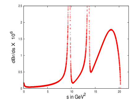
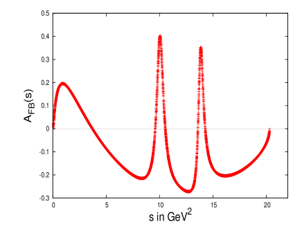
Figure 4: The differential branching ratio $d$Br/$ds$ versus $s$ (left panel) and the forward backward asymmetry ($A_{FB}(s)$) versus $s$ (right panel) for the process $\Lambda_{b}\to\Lambda\mu^{+}\mu^{-}$.

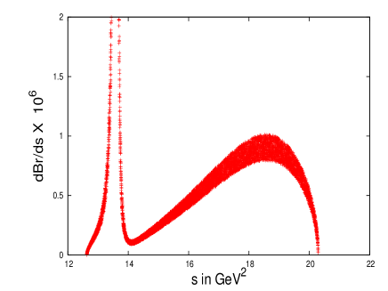
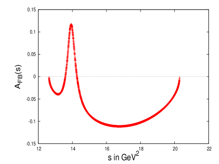
Figure 5: Same as Figure-4 for the process $\Lambda_{b}\to\Lambda\tau^{+}\tau^{-}$.

As discussed earlier in the presence of fourth generation, the Wilson coefficients $C_{7,9,10}$ will be modified due to the new contributions arising from the virtual $t^{\prime}$ quark in the loop. Thus, these coefficients will be modified as

$$C_{7}^{\rm tot}(\mu) = C_{7}(\mu)+\frac{\lambda_{t^{\prime}}}{\lambda_{t}}C_{7}^{\prime}(\mu),$$

$$C_{9}^{\rm tot}(\mu) = C_{9}(\mu)+\frac{\lambda_{t^{\prime}}}{\lambda_{t}}C_{9}^{\prime}(\mu),$$

$$C_{10}^{\rm tot}(\mu) = C_{10}(\mu)+\frac{\lambda_{t^{\prime}}}{\lambda_{t}}C_{10}^{\prime}(\mu).$$ (45)

The new coefficients $C_{7,9,10}^{\prime}$ can be calculated at the $M_{W}$ scale by replacing the $t$-quark mass by $m_{t}^{\prime}$ in the loop functions. These coefficients then to be evolved to the $b$ scale using the the renormalization group equation as discussed in buras1 . The values of the new Wilson coefficients at the $m_{b}$ scale for $m_{t^{\prime}}=400$ GeV is given by $C_{7}^{\prime}(m_{b})=-0.355$, $C_{9}^{\prime}(m_{b})=5.831$ and $C_{10}^{\prime}=-17.358$.

Thus, one can obtain the differential branching ratio and the forward backward asymmetry in SM4 by replacing $C_{7,9,10}$ in Eqs (41) and (44) by $C_{7,9,10}^{\rm tot}$. Using the values of the $|\lambda_{t}^{\prime}|$ and $\phi_{s}$ for $m_{t^{\prime}}=400$ GeV, differential branching ratio and the forward backward asymmetry for $\Lambda_{b}\to\Lambda\mu^{+}\mu^{-}$ is presented in Figure-6, where we have not considered the contributions from intermediate charmonium resonances. From the figure it can be seen that the differential branching ratio of this mode is significantly enhanced from its corresponding SM value whereas the forward backward asymmetry is slightly reduced with respect to its SM value. However, the zero-position of the FB asymmetry remains unchanged the fourth quark generation model. Similarly for the process $\Lambda_{b}\to\Lambda\tau^{+}\tau^{-}$ as seen from Figure-7, the branching ratio significantly enhanced from its SM value whereas the FB asymmetry remains almost unaffected in the SM4.

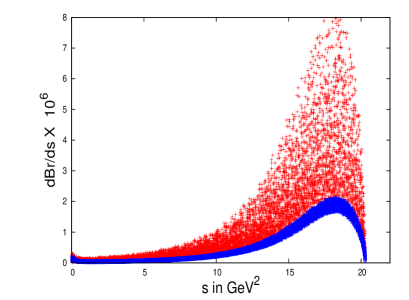
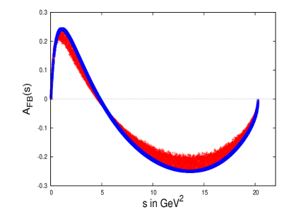
Figure 6: Variation of the differential branching ratio (left panel) and the forward-backward asymmetry (right panel) with respect to the momentum transfer $s$ for the process $\Lambda_{b}\to\Lambda\mu^{+}\mu^{-}$, in fourth quark generation model (red regions) whereas the corresponding SM values are shown by blue regions.

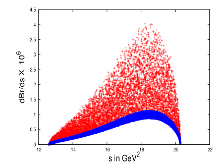
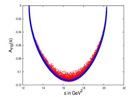
Figure 7: Same as Figure-6 for the process $\Lambda_{b}\to\Lambda\tau^{+}\tau^{-}$.

Table 4: The branching ratios (in units of $10^{-6}$) for various decay processes.

Decay modes	${\rm Br}^{\rm SM}$	${\rm Br}^{\rm SM4}$
$~{}\Lambda_{b}\to\Lambda\mu^{+}\mu^{-}$	13.25	($14.7\to 53.5$)
$\Lambda_{b}\to\Lambda\tau^{+}\tau^{-}$	3.83	( $4.3\to 16.0)~{}$

We now proceed to calculate the total decay rates for $\Lambda_{b}\to\Lambda~{}l^{+}l^{-}$ for which it is necessary to eliminate the backgrounds coming from the resonance regions. This can be done by by using the following veto windows so that the backgrounds coming from the dominant resonances $\Lambda_{b}\to\Lambda J/\psi(\psi^{\prime})$ with $J/\psi(\psi^{\prime})\to l^{+}l^{-}$ can be eliminated,

$$\Lambda_{b}\to\Lambda~{}\mu^{+}\mu^{-}: m_{J/\psi}-0.02<m_{\mu^{+}\mu^{-}}<m_{J/\psi}+0.02;$$

$$: m_{\psi^{\prime}}-0.02<m_{\mu^{+}\mu^{-}}<m_{\psi^{\prime}}+0.02$$

$$\Lambda_{b}\to\Lambda~{}\tau^{+}\tau^{-}: m_{\psi^{\prime}}-0.02<m_{\tau^{+}\tau^{-}}<m_{\psi^{\prime}}+0.02\;.$$

Using these veto windows we obtain the branching ratios for semileptonic rare $\Lambda_{b}$ decays which are presented in Table-4. It is seen from the table that the branching ratios obtained in the model in the fourth quark generation model are reasonably enhanced from the corresponding SM values and could be observed in the LHCb experiment.

V Conclusion

In this paper we have studied several rare decays of $\Lambda_{b}$ baryon, i.e., $\Lambda_{b}\to\Lambda\pi$, $\Lambda_{b}\to pK^{-}$, $\Lambda_{b}\to\Lambda\gamma$ and $\Lambda_{b}\to\Lambda l^{+}l^{-}$ in the fourth quark generation model. This model is a very simple extension of the standard model with three generations and it provides a simple explanation for the several indications of new physics that have been observed involving CP asymmetries in the $B$, $B_{s}$ decays for $m_{t}^{\prime}$ in the range of (400-600) GeV. We found that in this model the branching ratios of the various decay modes considered here ($\Lambda_{b}\to\Lambda\pi$, $\Lambda_{b}\to pK^{-}$, $\Lambda_{b}\to\Lambda\gamma$ and $\Lambda_{b}\to\Lambda l^{+}l^{-}$) are significantly enhanced from their corresponding SM values. However the forward backward asymmetries in the $\Lambda_{b}\to\Lambda~{}l^{+}l^{-}$ processes do not differ much from those of the SM expectations. The zero-point of the $F_{AB}$ for $\Lambda_{b}\to\Lambda~{}l^{+}l^{-}$ process is also found to be unaffected in this model.

Acknowledgments

The work of RM was partly supported by the Department of Science and Technology, Government of India, through Grant No. SR/S2/RFPS-03/2006.

References

(1) Heavy Flavor Averaging Group,
http://www.slac.stanford.edu/xorg/hfag.
(2) C. Amsler et al., Particle Data Group, Review of
Particle Physics, Phys. Lett. B
667, 1 (2008).
(3) M. Bona et al, [UT Fit Collaboration], JHEP 0803,049 (2008), [arXiv:0707.0636].
(4) T. E. Browder et al, Rev. Mod. Phys. 81, 1887 (2009), [arXiv:0802.3201].
(5) E. Lunghi and A. Soni, JHEP 0709, 053
(2007).
(6) A. Lenz and U. Nierste,
JHEP 0706, 072 (2007) ; A. Lenz, U. Nierste, J. Charles, S.
Descotes-Genon, A. Jantsch,
C. Kaufhold, H. Lacker, S. Monteil and V. Niess,
arXiv:1008.1593 [hep-ph].
(7) K. Agashe, G. Prerez and A. Soni, Phys. Rev. Lett. 93,
201804 (2004); Phys. Rev. D 71, 016002 (2005); M. Blanke et al, JHEP 0903, 001 (2009); M. Blanke et al, JHEP
0903, 108 (2009); V. Barger et al, JHEP 0912, 048
(2009); R. Mohanta and A. K. Giri, Phys. Rev. D 78, 116002
(2008), arXiv:0812.1077 [hep-ph]; ibid.79, 057902
(2009), arXiv:0812.1842 [hep-ph].
(8) W. -S. Hou, A. Soni and H. Steger, Phys. Lett. B 192, 441 (1987); W. S. Hou, R. S. Willey and A. Soni, Phys. Rev.
Lett. 58, 1608 (1987).
(9) J. Carpenter, R. Norton, S. Siegemund-Broka and A.
Soni, Phys. Rev. Lett. 65, 153 (1990); B. Holdom, Phys. Rev.
Lett. 57, 2496 (1986); Erratum- ibid58, 177
(1987); C T hill and E H Simmons. Phys. Rept. 381, 235
(2003); Erratum-ibid390, 553 (2004); B. Holdom, JHEP
0608, 076 (2006); G. Burdman, L. Da Rold, O. Eboli and R.
Matheus. Phys. Rev. D 79, 075026 (2009).
(10) W. -S. Hou, M. Nagashima and A.
Soddu, Phys. Rev. Lett 95, 141601 (2005); W. -S. Hou, H. -N.
Li, S. Mishima and M. Nagashima, Phys. Rev. Lett. 98, 131801
(2007); A. Arhrib and W. -S. Hou, Euro. Phys. J. C 27, 555
(2003); A. Arhrib and W. S. Hou, Phys. Rev. D 80, 076005
(2009); W. S. Hou, F. F. Lee, C. Y. Ma, Phys. Rev. D 79,
073002 (2009); W. S. Hou, M. Nagashima, A. Soddu, Phys. Rev. D 76, 016004 (2007); W. S. Hou, M. Nagashima, G. Raz and A. Soddu,
JHEP 0609, 012 (2006); Markus Bobrowski, Alexander Lenz,
Johann Riedl, J rgen Rohrwild, Phys. Rev. D. 79, 113006
(2009); O. Eberhardt, A. Lenz, J. Rohrwild, arXiv: 1005.3505
[hep-ph].
(11) A. Soni, A. Alok, A. Giri, R. Mohanta and S.Nandi,
Phys. Lett. B 683, 302 (2010), arXiv:0807.1971 [hep-ph]; Phys.
Rev. D. 82, 033009 (2010), arXiv:1002.0595 [hep-ph].
(12) A. J. Buras et al, arXiv:1002.2126 [hep-ph].
(13) Y. H. Chen, H. Y. Cheng, B. Tseng and K. C. Yang,
Phys. Rev. D 60, 094014 (1999).
(14) R. Mohanta, A. K. Giri and. M.P. Khanna, Phys. Rev. D
63, 074001 (2001), [arXiv:hep-ph/0006109].
(15) Y. M. Wang, Y. Li and C. D. Lu, Euro. Phys. C 59, 861 (2009), arXiv:0804.0648 [hep-ph];
Y. M. Wang, M. J. Aslam and C. D. Lu, Euro. Phys. C 59, 847
(2009), arXiv: 0810.0609 [hep-ph].
(16) S. Pakvasa, S. F. Tuan and S. P. Rosen, Phys. Rev. D
42, 3746 (1990).
(18) T. Inami and C. S. Lim, Prog. Theor. Phys. 65,
297 (1981); ibid65, 1772 (1981).
(19) G. Buchalla, A.J. Buras, M. Lautenbacher, Rev. Mod. Phys. 68, 1125 (1996).
(20) T. Aaltonen et al. (CDF Collaboration), Phys.
Rev. Lett. 103, 031801 (2009).
(21) Z. T. Wei, H. W. Ke and X. Q. Li, Phys. Rev. D 80, 094016 (2009).
(22) A. J. Buras and M. Münz, Phys. Rev. D 52, 186
(1995).
(23) T. M. Aliev, A. Ozpineci and M. Savci, Nucl.
Phys. B 649,
168 (2003); T. M. Aliev, A. Ozpineci and M. Savci, Phys. Rev. D 65, 115002 (2002); ibidD67, 035007 (2003);
Nucl. Phys. B 709, 115 (2005); T. M. Aliev, A. Ozpineci, M.
Savci and C. Yüce, Phys. Lett. B 542, 249 (2002); V.
Bashiry, K. Azizi, JHEP 0707, 064 (2007).
(24) M. Beneke, Th. Fledmann and D. Seidel, Nucl. Phys.
B 612, 25 (2001).
(25) C. S. Lim, T. Morozumi and A. I. Sanda, Phys. Lett. B.
218, 343 (1989); N. G. Deshpande, J. Trampetic and K. Ponose,
Phys. Rev. D 39, 1461 (1989); P. J. O’Donnell and H. K.K.
Tung, Phys. Rev. D 43, R2067 (1991); P. J. O’Donnell, M.
Sutherland and H. K.K. Tung, Phys. Rev. D 46, 4091 (1992); F.
Krüger and L. M. Sehgal, Phys. Lett. B 380, 199 (1996).
(26) R. Mohanta and A. K. Giri, Eur. Phys. C 45,
151 (2006); J. Phys. G 31, 1559 (2005).