Panchromatic Averaged Stellar Populations: paasp

Abstract

We study how the spectral fitting of galaxies, in terms of light fractions derived in one spectral region translates into another region, by using results from evolutionary synthesis models. In particular, we examine propagation dependencies on Evolutionary Population Synthesis (EPS, grasil, galev, Maraston and galaxev) models, age, metallicity, and stellar evolution tracks over the near-UV—near infrared (NUV—NIR, 3500Å to 2.5$\mu$m) spectral region. Our main results are: as expected, young ($t\lesssim$ 400 Myr) stellar population fractions derived in the optical cannot be directly compared to those derived in the NIR, and vice versa. In contrast, intermediate to old age ($t\gtrsim$ 500 Myr) fractions are similar over the whole spectral region studied. The metallicity has a negligible effect on the propagation of the stellar population fractions derived from NUV — NIR. The same applies to the different EPS models, but restricted to the range between 3800 Å and 9000 Å. However, a discrepancy between galev/Maraston and grasil/galaxev models occurs in the NIR. Also, the initial mass function (IMF) is not important for the synthesis propagation. Compared to starlight synthesis results, our propagation predictions agree at $\sim$95% confidence level in the optical, and $\sim$85% in the NIR. In summary, spectral fitting performed in a restricted spectral range should not be directly propagated from the NIR to the UV/Optical, or vice versa. We provide equations and an on-line form (Panchromatic Averaged Stellar Population - paasp) to be used for this purpose.

1 Introduction

A key issue in modern astrophysics is to understand how galaxies form and evolve, and the study of the stellar population and star formation history (over a wide wavelength range) may provide clues to the dominant mechanism. For example, two main scenarios are proposed to explain the formation of galaxies, one is the tidal torque theory, which suggests an initial collapse of gas at very high redshift (e.g. Eggen, Lynden-Bell & Sandage, 1962; White, 1984), and another is associated with galaxy mergers at intermediate to high redshifts (see Searle & Zinn, 1978; Hammer et al., 2005, 2007, 2009, for example). Both produce distinct signatures in the resulting stellar populations.

As we still cannot access the light of individual stars in almost any galaxy beyond the local group, the way widely used is to study the stellar populations by the integrated light of the whole galaxy or a significant fraction of it, by means of long-slit spectroscopy. The usual approaches for studying unresolved stellar populations are either by means of empirical population synthesis (Bica & Alloin, 1987; Bica, 1988; Bica et al., 1991; Bonatto et al., 1998, 2000; Cid Fernandes et al., 1998; Schmitt et al., 1996) or Evolutionary Population Synthesis (EPS) models (Bruzual & Charlot, 2003; Maraston, 1998, 2005; Vazdekis & Arimoto, 1999; Silva et al., 1998; Kotulla et al., 2009), as well as a combination of both techniques (Cid Fernandes et al., 2004, 2005; Riffel et al., 2007, 2008, 2009). By using them, we can infer the age and metallicity distributions of the stellar populations that make up a galaxy’s spectral energy distribution (SED).

The study of unresolved stellar populations in galaxies, ranging from star-forming to ellipticals, as well as in composite objects and active galaxies, is a common approach in the Near-UV (NUV) and optical bands (Bica, 1988; Schmitt et al., 1996; Cid Fernandes et al., 1998; González-Delgado et al., 1998; Bonatto et al., 1998, 2000; Raimann et al., 2003; González-Delgapickles98do et al., 2004; Cid Fernandes et al., 2005; Krabbe et al., 2008; Rickes et al., 2008, 2009). On the other hand, addressing unresolved stellar populations in the near infrared (NIR) is less common, starting $\sim$3 decades ago (Rieke et al., 1980, e.g.), but which seems to be in increasing expansion (Origlia, Moorwood & Oliva, 1993; Oliva et al., 1995; Engelbracht et al., 1998; Origlia & Oliva, 2000; Lançon et al., 2001; Davies et al., 2006, 2007, 2009; Riffel et al., 2007, 2008, 2009, 2010).

Very recently, Chen et al. (2010) have shown that using different EPS models in the optical leads to different stellar population results. So, it is not reasonable to directly compare stellar populations estimated from different EPS models. They suggest that to get reliable results, one should use the same EPS models to compare different samples. As related issues, can one compare the light-fraction results derived, with the same base of elements, in one spectral region to another? Are the population fractions derived in the optical the same in the NUV/NIR? What is the effect of the normalisation point used in the synthesis? Does the choice of elements that compose the base (i.e. age, metallicity and initial mass function - IMF) produce different results along the whole spectrum?

The answer to the above questions would be easy if stellar population synthesis were based on a more physical parameter, like mass-fractions. However, given the non-constant stellar mass-to-light ($M/L$) ratio, mass-fractions have a much less direct relation with the observables than light-fractions. In this context, we feel motivated to carry out a detailed study of the panchromatic averaged stellar population (paasp) components over the 3500Å to 2.5$\mu$m spectral region, commonly used for stellar population synthesis. It should be clear that paasp is not a tool for performing stellar population synthesis. Instead, it is specifically designed for translating the spectral fitting of galaxies (in terms of light fractions) derived in one spectral domain into another. This paper is structured as follows: The EPS models used are described in Sect. 2. The methodology and results are presented in Sect. 3. Results are discussed in Sect. 4. The final remarks are given in Sect. 5.

2 The adopted EPS models

In this section we describe the EPS models used in what follows. The four models: grasil, galev, Maraston and galaxev, have been selected because they have a spectral coverage from the NUV to the NIR region ($\sim$3500Å - 2.5$\mu$m) and are widely used. A brief description of them is made below. Details can be found in the original papers cited below, as well as in Chen et al. (2010).

2.1 grasil

The GRAphite and SILicate - grasil - code, developed by Silva et al. (1998), is a chemical evolution code that follows the star formation rate, metallicity and gas fraction, which are basic ingredients for stellar population synthesis. The latter is performed with a grid of integrated spectra of simple stellar populations (SSPs) of different ages and metallicities, in which the effects of dusty envelopes around asymptotic giant branch (AGB) stars are included, but not the AGB energetics (Bressan et al., 1998, 2002). The models consider four initial mass functions (IMFs), Kurucz (1992); Kennicutt et al. (1994); Scalo (1986); Miller & Scalo (1979). Kurucz (1992) atmosphere models, for population synthesis, and Padova tracks (Bertelli et al., 1994) are also considered. Moreover, SSPs of grasil cover a spectral range from 91Å up to 1200$\mu$m. Further details can be found in Laura Silva PhD thesis.

2.2 galev

The GALaxy EVolution - galev - evolutionary synthesis models describe the evolution of stellar populations in general, from star clusters to galaxies, both in terms of resolved stellar populations and integrated light properties (Kotulla et al., 2009). According to the authors, the code considers both the chemical evolution of the gas and the spectral evolution of the stellar component, allowing for a chemically consistent approach. Thus, some SSPs provided by galev show a emission line spectra.

The SSP models provided by galev cover 5 metallicities and 4000 ages ($\rm 0.02\leq Z/Z_{\odot}\leq 2.5$ and $\rm 4\,Myr\leq t\leq 16Gyr$). They are based on the spectra from BaSeL spectral library (Lejeune et al., 1997, 1999; Westera et al., 2002), originally based on the Kurucz (1992) library. They also have 3 different IMFs (Salpeter, 1955; Kroupa, 2001; Chabrier, 2003) and use the theoretical isochrones from the Padova team (e.g. Bertelli et al., 1994; Schulz et al., 2002). The wavelength coverage spans the range from 90Å to 160$\mu$m, with a spectral resolution of 20Å in the NUV-optical, and 50-100Å in the NIR. They also include the thermally- pulsating asymptotic giant branch (TP-AGB) phase provided by the Padova tracks (Schulz et al., 2002; Girardi et al., 2002). It is also worth mentioning at this point that the TP-AGB stars account for 25 to 40% of the bolometric light of an SSP, and for 40 to 60% of the light emitted in the K-band (e.g. Schulz et al., 2002; Maraston, 2005, and references therein). In addition, contrary to Maraston (2005, see below), galev models do not include empirical TP-AGB spectra. For a detailed description of galev see Kotulla et al. (2009).

2.3 Maraston models (M05)

The Maraston EPS models (hereafter M05) are being developed by Claudia Maraston since 1998 (Maraston, 1998) with an update in 2005 (Maraston, 2005). They are based on the fuel consumption theorem and include a proper treatment of the TP-AGB phase. According to these models, the effects of TP-AGB stars in the NIR spectra are unavoidable. The M05 models, by including empirical spectra of oxygen- and carbon-rich stars (Lançon & Wood, 2000), can predict the presence of NIR absorption features such as the 1.1$\mu$m CN band (Riffel et al., 2007, 2008, 2009), whose detection can be taken as an unambiguous evidence of a young to intermediate age SP. The models have been used by our team to study stellar populations in active galactic nuclei and starburst galaxies (Riffel et al., 2007, 2008, 2009, 2010, for CN, see also Ramos-Almeida et al. 2008 and Dottori et al. 2005) as well as in the age dating of massive galaxies at high redshift (Maraston et al., 2006; van der Wel et al., 2006; Rodighiero et al., 2007; Cimatti et al., 2008).

M05 models span a range of 6 different metallicities (${\rm\frac{1}{200}}\leq\frac{Z}{Z_{\odot}}\leq\rm 3.5$) with ages distributed from 1 Myr to 15 Gyr according to a grid of 67 models (Note that the full age grid is not available for all metallicities, M05). The IMFs considered are: Salpeter (1955) and Kroupa (2001). The stellar spectra were also taken from the BaSel library. The spectral range is from 91Å to 160$\mu$m, with a spectral a resolution of 5-10Å up to the optical region, and 20-100Å in the NIR. In Maraston (1998, 2005) models, the TP-AGB contributes with 40% to the bolometric flux, but rising to 80% when only the $K$-band is considered.

2.4 galaxev

galaxev is a widely used library of evolutionary stellar population synthesis models. It is computed with the isochrones synthesis code of Bruzual & Charlot (2003, also known as BC03) The spectral coverage of this library is from 91 Å up to 160$\mu$m, with a resolution of 3 Å between 3200 and 9500 Å, and a lower resolution elsewhere. Ages range from $\rm 1\times 10^{5}$ up to $\rm 2\times 10^{10}$ yr, for a wide range of metallicities (${\rm\frac{1}{200}}\lesssim\frac{Z}{Z_{\odot}}\lesssim\rm 2.5$). These models use the STELIB/BaSeL libraries (see Lejeune et al., 1997, 1999; Westera et al., 2002, and references therein) as well as the STELIB/Pickles libraries (Pickles, 1998). galaxev allows the use of two IMFs (Chabrier, 2003; Salpeter, 1955) and 3 stellar evolution tracks: Geneva (Schaller et al., 1992), Padova 94 (Alongi et al., 1993; Bressan et al., 1993; Fagotto et al, 1994a, b; Girardi et al., 1996) and Padova 00 (Girardi et al., 2000). These models do not include the TP-AGB phase.

3 Methodology and Results

First, we investigate the dependence of the stellar population components on the normalisation point, from the NUV to the NIR. To do this, we select spectral regions free from emission/absorption lines to be used as normalisation points, $F_{\lambda}$. They are: 3800Å  4020Å  4570Å  5300Å  5545Å  5650Å  5800Å  5870Å  6170Å 6620Å  8100Å  8815Å  9940Å  1.058$\mu$m 1.223$\mu$m 1.520$\mu$m 1.701$\mu$m 2.092$\mu$m 2.19$\mu$m (Bica, 1988; Rickes et al., 2008, 2009; Cid Fernandes et al., 2004; Saraiva et al., 2001; Riffel et al., 2008).

In addition, we select SSPs with ages: 0.005, 0.025, 0.050, 0.1, 0.2, 0.3,0.4 0.5,0.6, 0.7, 0.8, 0.9, 1.0, 2.0, 5.0 and 13 Gyr as representative of the stellar populations observed in galaxies. As a first exercise we combine two components: 13 Gry (the old population) and one of the other SSPs representing the “young” population. The combination was made by summing up, along the whole spectral range ($\sim$3500Å to 2.5$\mu$m), increasing fractions of the “young” component from 1 to 100%, according to

$$F=\left(1-f\right)F_{\rm y}+fF_{\rm o};$$ (1)

where $f$ is the fractional flux, which we vary in steps of 0.01, $F_{\rm y}$ is the flux of spectrum of the “young” component, for each $\lambda$ between $\sim$3500Å to 2.5$\mu$m, normalised to unity at 5870Å for the optical, or at 1.223$\mu$m for the NIR, and $F_{\rm o}$ is the flux of the 13 Gyr spectrum also normalised at the same points. Note that the normalisation of the spectra is done by dividing their fluxes by that of the normalisation point (5870Å or 1.223$\mu$m), after the computations are done. In addition, by normalising the spectra we are dealing with light-fractions, which are directly related to the observations. $\rm F$ is the resulting flux of the combined SSPs (young + old) at a specific $\lambda$. The averaged stellar population components spread over all $F_{\lambda}$ were derived by:

$$f_{\rm y}=\frac{(1-f)F_{\rm y}}{F}\ {\rm and}\ f_{\rm o}=\frac{fF_{\rm o}}{F}\$$ (2)

Eq.2 represents the young and old light fractions for different $F_{\lambda}$, this is what we call fraction at $\lambda$. The result of such process is summarised in Figs. 1 and 2. In these figures we show the sum of a “young” component with a 13 Gyr SSP (the old component) in steps of 10%. In practice we start with 5% of the flux of the “young” SSP + 95% of the flux of the 13 Gyr SSP, and finish with 95% of the young + 5% of the old component. This procedure is done over all $\lambda$s between the NUV and NIR. It is worth mentioning that Figs. 1 and 2, show M05 EPS models as reference (Sec. 4). These figures suggest that one cannot directly compare the light fractions of the young component ($t\lesssim$ 400 Myrs) derived in the optical with those obtained in the NIR, and vice versa (i.e. 77% of the 5 Myr population at 3800Å represents only 5% at 1.223$\mu$m). However, the intermediate to old components ($t\gtrsim$ 500 Myrs) can be directly compared between different wavelengths. This does not occur when dealing with mass fractions, since the age derived by the mass fraction is a more physical parameter, but has a much less direct relation with the observables, depending strongly on the $M/L$ ratio, which is not constant. Thus, the light fraction can be taken as an direct observable parameter and use Eqs. 1 and 2, to propagate the results over other spectral regions (see Appendix A).

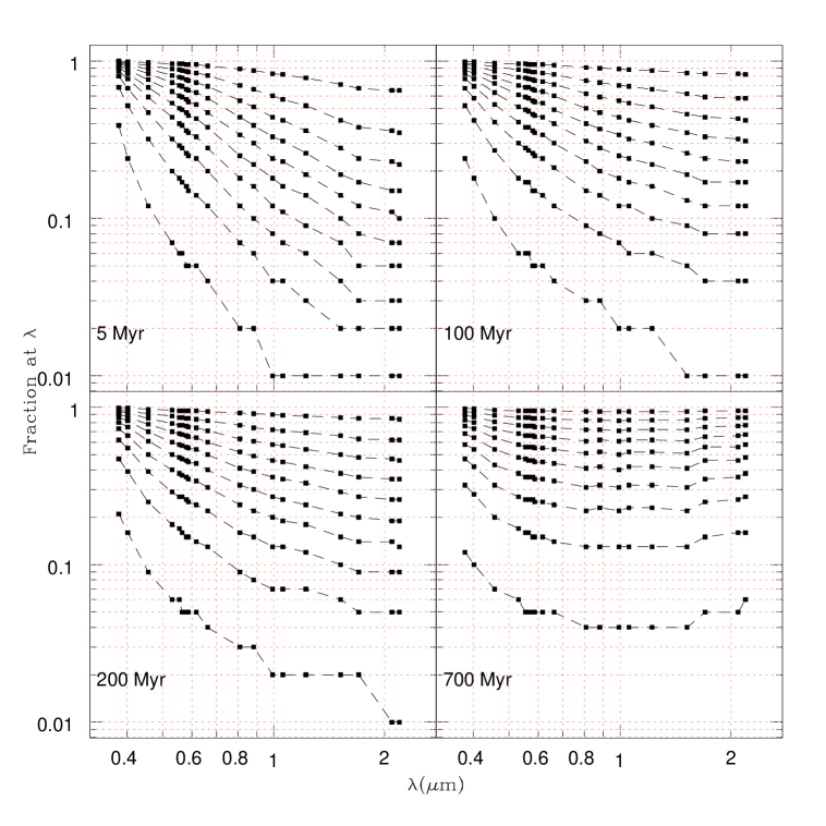
Figure 1: Light-fraction at $\lambda$ for the stellar population components. The curves result from Eq.2 with increasing fractions of 10% of the “young” component from bottom to top. In each panel we start with 5% of the flux of the “young” SSP + 95% of the 13 Gyr SSP, and finish with 95% of the young + 5% of the old component. The ages of the “young” component are on the labels. The normalisation point for the combination was 5870Å. We use the M05 models as reference. See text for more details.

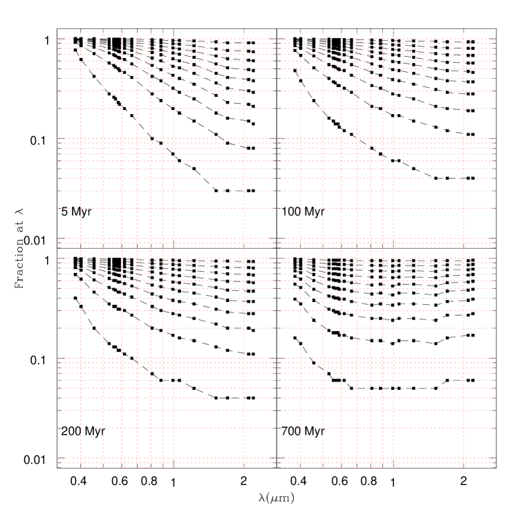
Figure 2: Same as Fig. 1 for the normalisation point at 1.223$\mu$m.

However, the stellar population of galaxies is not so simple as two components. Therefore, we have divided our SSPs into 3 population vectors $x_{y}$=0.005 Gyr; $x_{i}$=0.025…1.0 Gyr and $x_{o}$=13 Gyr. To investigate the effect of adding one more component to the above exercise, we combined three population vectors according to:

$$F^{\prime}=\frac{1}{100}\left(\gamma F_{\rm y}+\delta F_{\rm i}+\eta F_{\rm o}\right);$$ (3)

$${\rm with}\ \ \ \gamma+\delta+\eta=100$$

where, $\gamma$, $\delta$ and $\eta$ are the fractional fluxes from 0% to 100%, which are varied in steps of 1%; $F_{\rm y}$, $F_{\rm i}$ and $F_{\rm o}$ are the normalised fluxes (at $\lambda$=5870Å or $\lambda$ 1.223$\mu$m) of the $x_{\rm y}$, $x_{\rm i}$ and $x_{\rm o}$ population vectors, respectively. $\rm F^{\prime}$ is the resulting flux of the combined SSPs (young + intermediate + old) at a specific $\lambda$.

The averaged stellar population components distributed over all $\lambda$s were derived similarly to Eq. 2:

$$f^{\prime}_{\rm y}=\frac{\gamma F_{\rm y}}{F^{\prime}};\ \ \ f^{\prime}_{\rm i}=\frac{\delta F_{\rm i}}{F^{\prime}}\ \ \ {\rm and}\ \ \ f^{\prime}_{\rm o}=\frac{\eta F_{\rm o}}{F^{\prime}}\$$ (4)

We show the result of such combination in Figs. 4 to 5. It is clear that even with three population vectors, the results derived in one wavelength are not the same as in other $\lambda$s. In addition, Fig. 5 reinforces the fact that in the case of only intermediate to old components, the population fractions derived in one wavelength are nearly the same as in other $\lambda$s (i.e. the values derived in the optical can be used in the NIR).

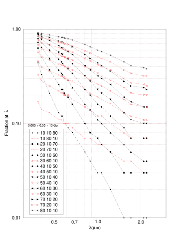
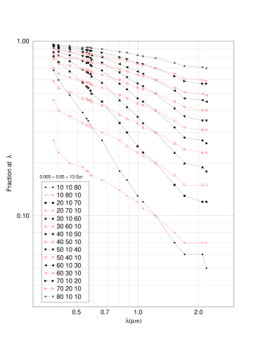
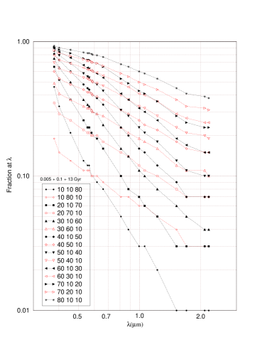
Figure 3: Light-fraction at $\lambda$ for the stellar population components.The curves result from Eq.4 with increasing fractions from bottom to top in each panel. The ages and the percentage fluxes are on the labels. The 5 Myr fraction increases from bottom to top. The normalisation points are 5870Å (left panel) and 1.223$\mu$m (right panel). We use the M05 models as reference.

Figure 4: Same as Fig. 4 for a different set of ages.

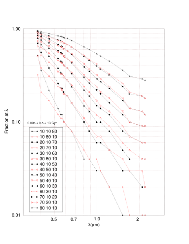
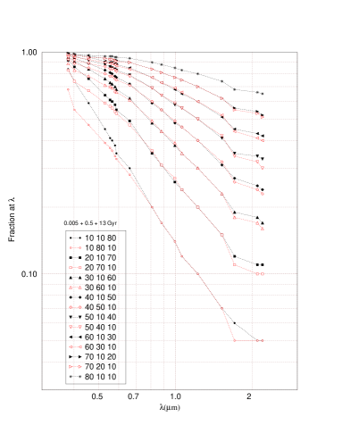
Figure 5: Same as Fig. 4 for a different set of ages.

4 Discussion

The determination of mean ages and metallicities of galaxies is important for models of galaxy formation and evolution. The techniques for dating unresolved stellar populations in local galaxies have focused on colours or spectroscopic indices measured in the NUV and optical (e.g. Bica, 1988; Worthey, 1994; Bica et al., 1996; Bonatto et al., 1996, 1998; Trager et al, 2000a, b; Maraston & Thomas, 2000; Thomas et al., 2005; Rickes et al., 2008, and references therein). However, even small mass fractions of young stars added to an old population can affect the NUV and optical age determinations significantly, making the galaxy appear young, which leads to a further degeneracy between mass fraction and age (Thomas & Davies, 2006; Serra & Trager, 2007). These problems may be solved for intermediate-age stellar populations looking in NIR wavelengths. In addition, the detection of young stellar populations in the NIR requires a hard work (Riffel et al., 2010). Nevertheless, it is clear from Fig. 2 that even a small fraction of a 5 Myr population ($\sim$ 5%) detected in the NIR may be responsible for almost all the light observed in the NUV ($\sim$ 70%).

Clearly, synthesis results should not be directly propagated from the NIR to the NUV/Optical, or vice versa. Instead, Eqs. 2 to  4 should be used for this purpose. To help with such a comparison we have created an on-line form, the Panchromatic Averaged Stellar Population: paasp and make available for download the tables with the results of the above equations (see Appendix A).

Another important ingredient in stellar population fitting is the metallicities used. As shown by Chen et al. (2010), the results of the fitting have a weaker dependence on metallicity than age. The question which arises here is, does metallicity affect the propagation of the averaged stellar populations? We investigate this effect with M05 SSPs with 3 different metallicities ($\frac{1}{50}Z\odot$; $Z\odot$; and 2 $Z\odot$) and the same age grid as in Fig. 1. The results are shown in Figs. 6 and 7. Clearly the propagation of the contributions has a negligible dependence on metallicity. Thus, one can use the condensed population vectors proposed by Cid Fernandes et al. (2004, 2005) to propagate the fitting results over all $\lambda$s.

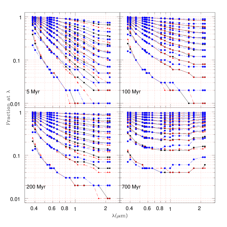
Figure 6: Metallicity effect for the normalisation point at 5870Å. Boxes represent solar metallicity, circles $\frac{1}{50}Z\odot$ and triangles are 2 $Z\odot$. We use the M05 models as reference.

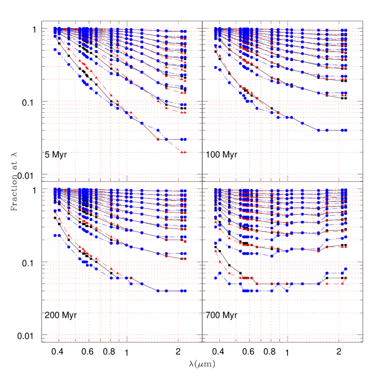
Figure 7: Same as Fig. 6 for the normalisation point at 1.223$\mu$m.

All the tests described above were made using the M05 models, but, as stated in Sec. 2, there are more EPS models available in the literature covering simultaneously the spectral region between $\sim$3500Å and 2.5$\mu$m. Thus, it is necessary to test if the selection of EPS models will produce different results in the propagation of the synthesis results over different $\lambda$s. In Fig. 8 we compare the different models among each other. It is clear that in the case of the optical normalisation point (5870Å), the four models produce very similar results in the interval between 3800 Å and 9000 Å, but a discrepancy between galev/M05 and grasil/BC03 models is observed in the NIR. Such a discrepancy is due to the well known fact that galev and M05 models do include stars in the TP-AGB phase (see M05, for example), which is more sensitive to the NIR than the optical, i.e TP-AGB stars account for 25 to 40% of the bolometric light of an SSP, and for 40 to 60% of the light emitted in the K-band (see Schulz et al., 2002; Maraston, 2005, and references therein). However, there is a difference between galev and M05 models, enhanced in the 100 Myr population. There are two possible explanations for this discrepancy: one is associated with the different onset age of the TP-AGB on the models. A high TP-AGB contribution at 100 Myr, as applied by Schulz et al. (2002), which is excessively high when compared to young Large Magellanic Cloud globular clusters (Maraston, 1998; Marigo et al., 2008). The other is associated with the way in which the TP-AGB treatment is made (Maraston et al., 2006; Bruzual, 2007). galev includes TP-AGB by means of isochrones (Padova94 + improved TP-AGB models Bertelli et al., 1994; Girardi et al., 2000; Marigo et al., 2008), while M05 is based on a different approach, the fuel consumption theorem. According to Maraston (2005), the stellar luminosity during the evolutionary phases that follow or suffer from mass loss cannot be predicted by stellar tracks, because there is no theory linking mass-loss rates to the basic stellar parameters, such as luminosity.

Note that the trend observed in Fig. 8 can also be associated with the fact that in M05 models, the TP-AGB contributes with 40% to the bolometric flux, and 80% to the K-band. This is higher than the “simpler” calculations (made by the Padova group at the time) used by Schulz et al. (2002), in which only some thermal pulses have been included (Girardi et al., 2000).

In addition, the tests were performed with the Salpeter (1955) IMF. To see the effect of the IMF on the averaged stellar populations over all $\lambda$s, we repeat the same exercises for different IMFs and summarise the results in Fig. 10. This figure suggests that the IMF does not play an important role in the synthesis propagation to other spectral regions.

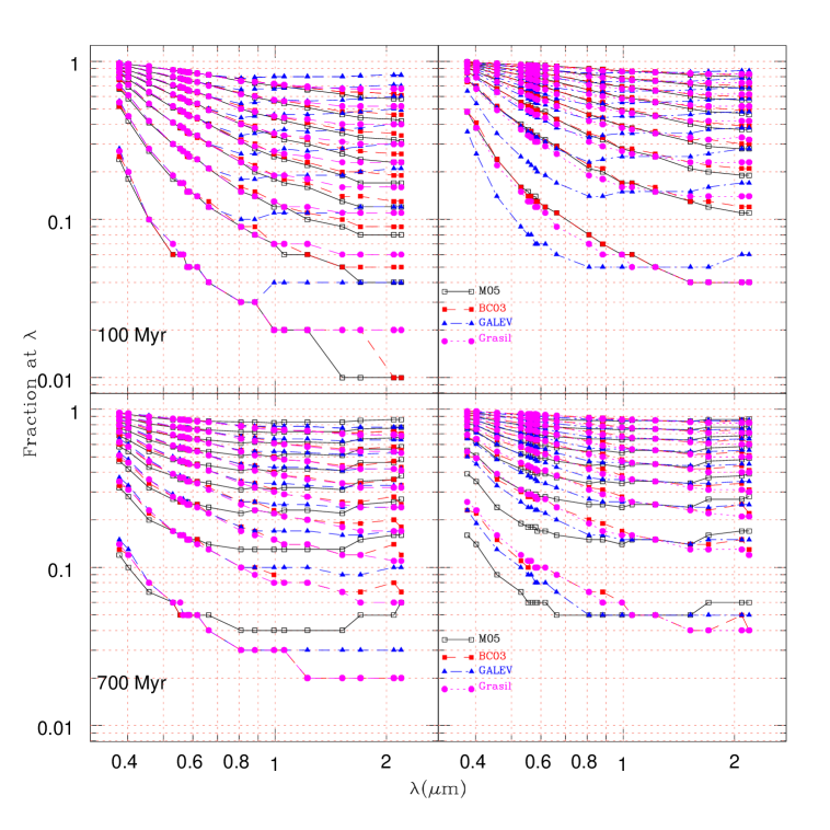
Figure 8: Comparison of different EPS models. Normalised at 5870Å (left) and 1.223$\mu$m(right). Note that we use 100 Myr + 13 Gyr SSPs.

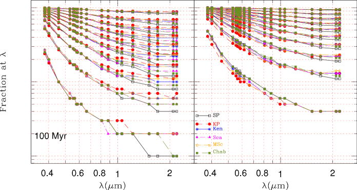
Figure 9: Effect of different IMFs. At left the normalisation point is 5870Å and at right 1.223$\mu$m. Salpeter (SP) and Kroupa (KP) where taken from M05 models; Kennicutt (Ken), Scalo (Sca) and Miller & Scalo (MSc) IMFs were taken from grasil EPS and Chabrier (Chab) are from galaxev.

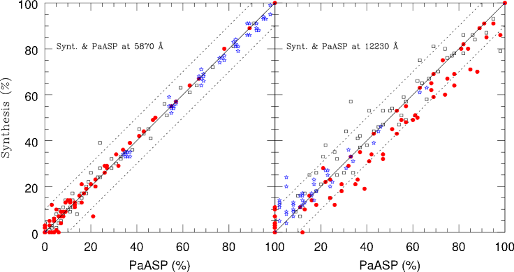
Figure 10: paasp tests. Stars, boxes and circles represent the 5 Myr, 700 Myr and 13 Gyr SSPs, respectively. Identity is shown by the solid line and dotted lines indicate the 90% confidence level.

4.1 Testing paasp

In order to test if we are able to predict the averaged stellar populations over all lambdas, extensive simulations were performed to evaluate the paasp’s ability to recover input parameters. In short, we build artificial galaxy spectra by mixing Maraston (2005) solar metallicity SSP models of 5 Myr, 700 Myr and 13 Gyr in different proportions, and perform stellar population synthesis with normalisation points at the optical (5870Å) and NIR (12230Å). To this purpose we use the starlight code optimised to the optical region (Cid Fernandes et al., 2004, 2005; Mateus et al., 2006; Asari et al., 2007; Cid Fernandes et al., 2008), and which also produces reliable results when applied to the NIR spectral (Riffel et al., 2009, 2010).

In summary, starlight fits an observed spectum $O_{\lambda}$ with a combination, in different proportions, of $N_{*}$ SSPs. Basically, it solves the following equation (Cid Fernandes et al., 2005):

$$M_{\lambda}=M_{\lambda 0}\left[\sum_{j=1}^{N_{*}}x_{j}\,b_{j,\lambda}\,r_{\lambda}\right]\otimes G(v_{*},\sigma_{*}),$$ (5)

where $M_{\lambda}$ is a model spectrum, $b_{j,\lambda}\,r_{\lambda}$ is the reddened spectrum of the $j$th SSP normalised at $\lambda_{0}$; $r_{\lambda}=10^{-0.4(A_{\lambda}-A_{\lambda 0})}$ is the reddening term; $M_{\lambda 0}$ is the synthetic flux at the normalisation wavelength; $\vec{x}$ is the population vector; $\otimes$ denotes the convolution operator, and $G(v_{*},\sigma_{*})$ is the Gaussian distribution used to model the line-of-sight stellar motions, which is centred at velocity $v_{*}$ with dispersion $\sigma_{*}$. The final fit is carried out with a simulated annealing plus Metropolis scheme, which searches for the minimum of the equation:

$$\chi^{2}=\sum_{\lambda}[(O_{\lambda}-M_{\lambda})w_{\lambda}]^{2},$$ (6)

where emission lines and spurious features are masked out by fixing $w_{\lambda}$=0. For a detailed description of starlight see Cid Fernandes et al. (2004, 2005).

As base set we take Maraston (2005) SSPs covering 14 ages, $t$= 0.001, 0.005, 0.01, 0.03, 0.05, 0.1, 0.2, 0.5, 0.7, 1, 2, 5, 9, 13 Gyr, and 4 metallicities, namely: $Z$= 0.02 $Z_{\odot}$, 0.5 $Z_{\odot}$, 1 $Z_{\odot}$ and 2 $Z_{\odot}$, summing up 56 elements.

To compare starlight with paasp predictions, we use the condensed population vector, which is obtained by binning the synthesis results into young, $x_{Y}$ ($t\leq\rm 5\times 10^{7}$yr); intermediate-age, $x_{I}$ ($1\times 10^{8}\leq t\leq\rm 2\times 10^{9}$yr) and old, $x_{O}$ ($t>\rm 2\times 10^{9}$yr) components (Riffel et al., 2009; Cid Fernandes et al., 2004). These components were then taken to represent the 5 Myr, 700 Myr and 13 Gyr old populations. These vectors are compared with the paasp predictions in Fig. 10.

Clearly, our predictions are consistent with the stellar population synthesis, especially at the optical region, where the confidence level between predictions and synthesis is $\sim$95% (i.e. almost all points fall in a region less than 5% from the identity line). The confidence level drops to $\sim$85% in the NIR.

5 Final Remarks

We study the panchromatic stellar population components over the 3500Å to 2.5$\mu$m spectral region. In particular, we analyse how the spectral fitting of galaxies based on light-fractions derived in a given spectral range can be propagated over all $\lambda$s. Dependencies on EPS models, age, metallicity, and stellar evolution tracks of four widely used EPS models (grasil, galev, Maraston and galaxev) were taken into account. Our main results are:

• The young ($t\lesssim$ 400 Myr) stellar population fractions derived in the optical cannot be directly compared to those derived in the NIR, and vice versa. For example, a contribution of $\sim$ 80% of a 5 Myr population at 3800Å translates into only 5% at 1.223$\mu$m.

• The intermediate to old age components ($t\gtrsim$ 500 Myr) can be directly compared from the NUV up to the NIR.

• The metallicity dependence on the propagation of the stellar population fractions derived from NUV — NIR is negligible.

• Different EPS models produce similar results in the propagation of the synthesis results over the interval between 3800 Å and 9000 Å. However, a discrepancy between galev/M05 and grasil/BC03 models occurs in the NIR. Such a discrepancy may be due to the fact that galev and M05 models do include stars in the TP-AGB phase.

• There is a difference between galev and M05 models, enhanced in the 100 Myr population. Such a discrepancy may be associated with the way in which the TP-AGB treatment is made (Maraston et al., 2006; Bruzual, 2007).

• We test the effect of 6 different IMFs, and we conclude that the IMF is not important in the propagation of the synthesis results.

• Extensive simulations were performed to evaluate paasp’s ability to recover input parameters. Our predictions are consistent with the stellar population synthesis with a confidence level between the predictions and synthesis of $\sim$95% in the optical and $\sim$85% in the NIR.

  In summary, spectral fitting results should not be directly propagated from the NIR to the NUV/Optical, or vice versa. Instead, Eqs. 2 to  4 should be used for this purpose. However, since this is hard to do when dealing with large samples of objects, we have created an on-line form, the Panchromatic Averaged Stellar Population - paasp, available at: http://www.if.ufrgs.br/$\sim$riffel/software.html. We also make available for download the tables with the results of the above equations for a wide range of ages (see Appendix  A).

Appendix A How to use the paasp form

In this appendix we provide details how to use the paasp form. paasp is available at http://www.if.ufrgs.br/$\sim$riffel/software.html.

1. Bin your synthesis results ($\vec{x_{j}}$) into 3 population vectors: young, intermediate, and old ages. For more information on the definition of the populations vectors see Cid Fernandes et al. (2004, 2005) and Riffel et al. (2009).

2. Select the representative age of each vector, for example: 5 Myr for young, 200 Myr for intermediate, and 13 Gyr for old. Tip: take as the representative population the ages of $\vec{x_{j}}$ with the largest contribution in each bin.

3. Put the percentage contribution (only integers and sum equal to 100% are allowed) of each age in the form, select the normalisation point and submit it.

4. You will be redirected to the results query page. There your inputs are marked in red and the propagated results over all $\lambda$s (see text) are shown. You can also download the file with a table with propagation results for all the results of Eq. 4, in fractions of 1% for your query.

5. The 3 first columns of the table are the input fractions for a given normalisation point and for 3 ages, which are specified in the header (first and second lines). The next columns are the propagation of the results for all $\lambda$s. Note that the results are given in 3 lines blocks: young, intermediate and old fractions, respectively.

   paasp  is freely distributed and is supported by Brazilian funding agencies CAPES and CNPq. An acknowledgement for the use would be appreciated.

References

- Alongi et al. (1993) Alongi, M., Bertelli, G., Bressan, A., et al. 1993, A&AS, 97, 851
- Asari et al. (2007) Asari, N. V., Cid Fernandes, R., Stasińska, G., Torres-Papaqui, J. P., Mateus, A., Sodré, L., Schoenell, W., Gomes, J. M., 2007, MNRAS, 381, 263
- Bonatto et al. (1996) Bonatto, C.; Bica, E.; Pastoriza, M. G.& Alloin, D.,
- Bonatto et al. (2000) Bonatto, C., Bica, E., Pastoriza, M. G. & Alloin, D., 2000, A&A, 355, 99
- Bonatto et al. (1998) Bonatto, C., Pastoriza, M. G., Alloin, D., Bica, E., 1998, A&A, 334, 439
- Bica & Alloin (1987) Bica, E. & Alloin, D., 1987, A&A, 186, 49.
- Bica (1988) Bica, E. 1988, A & A, 195, 9.
- Bica et al. (1991) Bica, E., Pastoriza, M. G., da Silva, L. A. L., Dottori, H., Maia, M., 1991, AJ, 102, 1702
- Bica et al. (1996) Bica, E.; Bonatto, C.; Pastoriza, M. G.& Alloin, D.,1996, A&A, 313, 405.
- Bertelli et al. (1994) Bertelli, G.; Bressan, A.; Chiosi, C.; Fagotto, F.; Nasi, E., 1994, A&AS, 106, 275.
- Bressan et al. (1993) Bressan, A., Fagotto, F., Bertelli & G., Chiosi, C. 1993, A&AS, 100, 647
- Bressan et al. (1998) Bressan, A., Granato, G.L., Silva, L., 1998, A&A, 332, 135
- Bressan et al. (2002) Bressan, A., Silva, L., Granato, G.L., 2002, A&A, 392, 377
- Bruzual & Charlot (2003) Bruzual, G. & Charlot, S., 2003, MNRAS, 344, 1000
- Bruzual (2007) Bruzual, G., 2007, From Stars to Galaxies: Building the Pieces to Build Up the Universe. ASP Conference Series, Vol. 374, proceedings of the conference held 16-20 October 2006 at Istituto Veneto di Scienze, Lettere ed Arti, Venice, Italy. Edited by Antonella Vallenari, Rosaria Tantalo, Laura Portinari, and Alessia Moretti., p.303
- Cid Fernandes et al. (1998) Cid Fernandes, R., J.., Storchi-Bergmann, T., Schmitt, H. R., 1998, MNRAS, 297, 579
- Cid Fernandes et al. (2004) Cid Fernandes, R., Gu, Q., Melnick, J., Terlevich, E., Terlevich, R., Kunth, D., Rodrigues Lacerda, R., Joguet, B., 2004, MNRAS, 355, 273
- Cid Fernandes et al. (2005) Cid Fernandes, R., Mateus, A., Sodré, Laerte, Stasińska, G., Gomes, J. M., 2005a, MNRAS, 358, 363 (CF05)
- Cid Fernandes et al. (2008) Cid Fernandes, R., Schoenell, W., Gomes, J. M., Asari, N
- Cimatti et al. (2008) Cimatti et al., 2008, A&A, 482, 21.
- Chabrier (2003) Chabrier, G. 2003, PASP, 115, 763
- Chen et al. (2010) Chen, X. Y.; Liang, Y. C.; Hammer, F.; Prugniel, Ph.; Zhong, G. H.; Rodrigues, M.; Zhao, Y. H.; Flores, H., 2010, arXiv: 1002.2013
- Davies et al. (2006) Davies, R. I.; Thomas, J.; Genzel, R.; Sánchez, F. Mueller; Tacconi, L. J.; Sternberg, A.; Eisenhauer, F.; Abuter, R.; Saglia, R.; Bender, R., 2006, ApJ, 646, 754.
- Davies et al. (2007) Davies, R. I.; Sánchez, F. Mueller; Genzel, R.; Tacconi, L. J.; Hicks, E. K. S.; Friedrich, S.; Sternberg, A., 2007, ApJ, 671, 1388.
- Davies et al. (2009) R. Davies, W. Maciejewski, E. Hicks, L. Tacconi, R. Genzel, H. Engel, 2009, arXiv:0903.0313.
- Dottori et al. (2005) Dottori, H., Díaz, R. J., Carranza, G., Lípari, S. & Santos, J., Jr., 2005, ApJ, 628L, 85.
- Engelbracht et al. (1998) Engelbracht, C. W., Rieke, M. J., Rieke, G. H., Kelly, D. M. & Achtermann, J. M., 1998, ApJ, 505, 639.
- Eggen, Lynden-Bell & Sandage (1962) Eggen, O. J., Lynden-Bell, D. & Sandage, A. R., 1962, ApJ, 136, 748.
- Fagotto et al (1994a) Fagotto, F., Bressan, A., Bertelli, G. & Chiosi, C. 1994a, A&AS, 104, 365
- Fagotto et al (1994b) Fagotto, F., Bressan, A., Bertelli, G. & Chiosi, C. 1994b, A&AS, 105, 29
- Girardi et al. (1996) Girardi, L., Bressan, A., Chiosi, C., Bertelli, G. & Nasi, E. 1996, A&AS, 117, 113
- Girardi et al. (2000) Girardi, L., Bressan, A., Bertelli, G. & Chiosi, C. 2000, A&AS, 141, 371
- Girardi et al. (2002) Girardi, L., Bressan, A., Bertelli, G., & Chiosi, C. 2000, A&AS, 141,371
- González-Delgado et al. (1998) González Delgado, R. M., Leitherer, C., Heckman, T., Lowenthal, J. D., Ferguson, H. C. & Robert, C., 1998, ApJ, 495, 698
- González-Delgapickles98do et al. (2004) González Delgado, R. M., Cid Fernandes, R., Pèrez, E., Martins, L. P., Storchi-Bergmann, T., Schmitt, H., Heckman, T., Leitherer, C.,2004, ApJ, 605, 127.
- Hammer et al. (2005) Hammer, F., Flores, H., Elbaz, D., et al. 2005, A&A, 430, 115.
- Hammer et al. (2007) Hammer, F., Puech, M., Chemin, L., Flores, H. & Lehnert, M. D., 2007, ApJ, 662, 322.
- Hammer et al. (2009) Hammer, F., Flores, H., Puech, M., et al. 2009, A&A, 507, 1313.
- Kennicutt et al. (1994) Kennicutt, Robert C., Jr.; Tamblyn, Peter; Congdon, Charles E., 1994, ApJ, 435,22.
- Krabbe et al. (2008) Krabbe, A. C.; Pastoriza, M. G.; Winge, C.; Rodrigues, I.; Ferreiro, D. L., 2008, MNRAS, 389, 1593.
- Kurucz (1992) Kurucz R. L. 1992, The Stellar Populations of Galaxies, ed. Barbuy, B. & Renzini, A. IAU Symp., 149, 225.
- Kotulla et al. (2009) Kotulla, R.; Fritze, U.; Weilbacher, P.; Anders, P., 2009, MNRAS, 396, 462.
- Kroupa (2001) Kroupa, P. 2001, MNRAS, 322, 231
- Lançon & Wood (2000) Lançon, A. & Wood, P. R. 2000, A&AS, 146, 217.
- Lançon et al. (2001) Lançon, A., Goldader, J. D., Leitherer, C., & González Delgado, R. M., 2001, ApJ, 552, 150
- Lejeune et al. (1997) Lejeune, Th., Cuisinier, F. & Buser, R. 1997, A&AS, 125, 229
- Lejeune et al. (1999) Lejeune, Th., Cuisinier, F. & Buser, R. 1998, A&AS, 130, 65
- Marigo et al. (2008) Marigo, P.; Girardi, L.; Bressan, A.; Groenewegen, M. A. T.; Silva, L.; Granato, G. L., 2008,A&A, 482, 883.
- Mateus et al. (2006) Mateus, A., Sodré, L., Cid Fernandes, R., Stasińska, G., Schoenell, W., Gomes, J. M., 2006, MNRAS, 370, 721
- Maraston (1998) Maraston, C., 1998, MNRAS, 300, 872.
- Maraston & Thomas (2000) Maraston, C. & Thomas, D., 2000, ApJ, 541, 126.
- Maraston (2005) Maraston, C., 2005, MNRAS, 362, 799 (M05).
- Maraston et al. (2006) Maraston, C., Daddi, E., Renzini, A., Cimatti, A., Dickinson, M., Papovich, C., Pasquali, A. & Pirzkal, N., 2006, ApJ, 652, 85.
- Miller & Scalo (1979) Miller, G. E.; Scalo, J. M., 1979, ApJS, 41, 513.
- Origlia, Moorwood & Oliva (1993) Origlia, L., Moorwood, A. F. M., Oliva, E., 1993,A&A, 280, 536.
- Oliva et al. (1995) Oliva, E., Origlia, L., Kotilainen, J. K., Moorwood, A. F. M., 1995, A&A, 301, 55.
- Origlia & Oliva (2000) Origlia, L. & Oliva, E., 2000, NewAR, 44, 257
- Pickles (1998) Pickles, A. J. 1998, PASP, 110, 863.
- Raimann et al. (2003) Raimann, D., Storchi-Bergmann, T., González Delgado, R. M., Cid Fernandes, R., Heckman, T., Leitherer, C., Schmitt, H., 2003, MNRAS, 339, 772.
- Ramos-Almeida et al. (2008) Ramos A., C.; Pérez G., A. M.; Acosta-Pulido & J. A.; González-Martin, O., 2008, ApJ, 680L, 17
- Rieke et al. (1980) Rieke, G. H., Lebofsky, M. J., Thompson, R. I., Low, F. J., Tokunaga, A. T., 1980, ApJ, 238, 24
- Rickes et al. (2009) Rickes, M. G.; Pastoriza, M. G.; Bonatto, C., 2009, A&A, 505, 73.
- Rickes et al. (2008) Rickes, M. G.; Pastoriza, M. G.; Bonatto, C., 2008, MNRAS, 384, 1427
- Riffel et al. (2007) Riffel, R., Pastoriza, M. G., Rodríguez-Ardila, A. & C. Maraston, 2007, ApJ, 659L, 103.
- Riffel et al. (2008) Riffel, R., Pastoriza, M. G., Rodríguez-Ardila, A. & C. Maraston, 2008b, MNRAS, 388, 803.
- Riffel et al. (2009) Riffel, R., Pastoriza, M. G., Rodríguez-Ardila, A. & C. Bonatto, 2007, 2009, MNRAS, 400, 273.
- Riffel et al. (2010) Riffel, Rogemar A.; Storchi-Bergmann, T.; Riffel, R.; Pastoriza, M., 2010, ApJ, 713, 469.
- Rodighiero et al. (2007) Rodighiero, G.; Cimatti, A.; Franceschini, A.; Brusa, M.; Fritz, J.; Bolzonella, M., 2007, A&A, 470, 21.
- Salpeter (1955) Salpeter, E. E. 1955, ApJ, 121, 161.
- Saraiva et al. (2001) Saraiva M. F., Bica E., Pastoriza M. G., Bonatto C., 2001, A&A, 376, 43
- Scalo (1986) Scalo, J. M., Luminous stars and associations in galaxies; Proceedings of the Symposium, Porto-Kheli, Greece, May 26-31, 1985 (A87-16301 04-90). Dordrecht, D. Reidel Publishing Co., 1986, p. 451-466.
- Schaller et al. (1992) Schaller, G., Schaerer, D., Meynet, G. & Maeder, A. 1992, A&AS, 96, 269
- Schulz et al. (2002) Schulz, J., Fritze, U., Moller, C. S., & Fricke, K. J. 2002, A&A, 392, 1.
- Schmitt et al. (1996) Schmitt, H. R., Bica, E., & Pastoriza, M. G. 1996, MNRAS, 278, 965
- Searle & Zinn (1978) Searle, L.; Zinn, R., 1978, ApJ, 225, 357.
- Serra & Trager (2007) Serra, P. & Trager, S. C., 2007, MNRAS, 374, 769.
- Silva et al. (1998) Silva, L., Granato, G.L., Bressan, A., Danese, L., 1998, ApJ, 509, 103.
- Taantalo et al. (1996) Tantalo, R.; Chiosi, C.; Bressan, A.; Fagotto, F., 1996, A&A, 311, 361.
- Thomas et al. (2005) Thomas, D.; Maraston, C.; Bender, R.; Mendes de Oliveira, C., 2005, ApJ, 621, 673.
- Thomas & Davies (2006) Thomas, D. & Davies, R. L., 2006, MNRAS, 366, 510.
- Trager et al (2000a) Trager, S. C.; Faber, S. M.; Worthey, Guy; González, J. Jesús, 2000a, AJ, 120, 165.
- Trager et al (2000b) Trager, S. C.; Faber, S. M.; Worthey, Guy; González, J. Jesús, 2000b, AJ, 119, 1645.
- Vazdekis & Arimoto (1999) Vazdekis, A. & Arimoto, N. 1999, ApJ, 525, 144.
- van der Wel et al. (2006) van der Wel, A.; Franx, M.; Wuyts, S.; van Dokkum, P. G.; Huang, J.; Rix, H.-W.; Illingworth, G. D., 2006, ApJ, 652, 97.
- White (1984) White, S. D. M. 1984, ApJ, 286, 38.
- Westera et al. (2002) Westera, P., Lejeune, T., Buser, R., Cuisinier, F. & Bruzual, G. 2002, A&A, 381, 524
- Worthey (1994) Worthey, G., 1994, ApJS, 95, 107.