Transit timing variations in eccentric hierarchical triple exoplanetary systems

Abstract

Aims. We study the long-term time-scale (i.e. period comparable to the orbital period of the outer perturber object) transit timing variations in transiting exoplanetary systems which contain a further, more distant ($a_{2}>>a_{1}$) either planetary, or stellar companion.

Methods. We give an analytical form of the $O-C$ diagram (which describes such TTV-s) in trigonometric series, valid for arbitrary mutual inclinations, up to the sixth order in the inner eccentricity.

Results. We show that the dependence of the $O-C$ on the orbital and physical parameters can be separated into three parts. Two of these are independent of the real physical parameters (i.e. masses, separations, periods) of a concrete system, and depend only on dimensionless orbital elements, and so, can be analysed in general. We find, that for a specific transiting system, where eccentricity ($e_{1}$) and the observable argument of periastron ($\omega_{1}$) are known e.g. from spectroscopy, the main characteristics of any, caused by a possible third-body, transit timing variations can be mapped simply. Moreover, as the physical attributes of a given system occur only as scaling parameters, the real amplitude of the $O-C$ can also be estimated for a given system, simply as a function of the $m_{3}/P_{2}$ ratio. We analyse the above-mentioned dimensionless amplitudes for different arbitrary initial parameters, as well as for two particular systems CoRoT-9b and HD 80606b. We find in general, that while the shape of the $O-C$ strongly varies with the angular orbital elements, the net amplitude (departing from some specific configurations) depends only weakly on these elements, but strongly on the eccentricities. As an application, we illustrate how the formulae work for the weakly eccentric CoRoT-9b, and the highly eccentric HD 80606b. We consider also the question of detection, as well as the correct identification of such perturbations. Finally, we illustrate the operation and effectiveness of Kozai cycles with tidal friction (KCTF) in the case of HD 80606b.

1 Introduction

The rapidly increasing number of exoplanetary systems, as well as the lengthening time interval of the observations naturally leads to the search for perturbations in the motion of the known planets which can provide the possibility to detect further planetary (or stellar) components in a given system, and/or can produce further information about the oblateness of the host star (or the planet), or might even refer to evolutionary effects.

The detection and the interpretation of such perturbations in the orbital revolution of the exoplanets usually depends on such methods and theoretical formulae which are well-known and have been applied for a long time in the field of the close eclipsing and spectroscopic binaries. We mainly refer to the methods developed in connection with the observed period variations in eclipsing binaries. These period variations manifests themselve in the departure of the occurrence of an eclipse event (either transit, or occultation) from its predicted time. Applying the nomenclature of exoplanet studies this phenomenon is called transit timing variation (TTV). Plotting the observed minus calculated mid-transit times with respect to the cycle numbers we get the $O-C$ diagram which has been the main tool for period studies by variable star observers (not only for eclipsing binaries) for more than a century. Consequently, the effect of the various types of period variations (both real and apparent) for the $O-C$ diagram were already widely studied in the last one hundred years. Some of these are less relevant in the case of transiting exoplanets, but others are important. For example, the two classical cases are the simple geometrical light-time effect (LITE) (due to a further, distant companion), and the apsidal motion effect (AME) (due to both the stellar oblateness in eccentric binaries and the relativistic effect). Due to its small amplitude however, LITE, which has been widely used for identification further stellar companions of many variable stars (not only in case of eclipsing binaries) since the papers of Chandler (1892); Hertzsprung (1922); Woltjer (1922); Irwin (1952), is less significant in the case of a planetary-mass wide component. Nevertheless in the recent years there have been some efforts to discover exoplanets on this manner (see e.g. Silvotti et al. 2007, V391 Pegasi, Deeg et al. 2008, CM Draconis, Qian et al. 2009, QS Virginis, Lee et al. 2009, HW Virginis). The importance of AME in close exoplanet systems has been investigated in several papers (see e.g. Miralda-Escudé 2002; Heyl & Gladman 2007; Jordán & Bakos 2008, and further references therein). Note, that this latter effect has been studied since the pioneering works of Cowling (1938); Sterne (1939), and besides its evident importance in the checking of the general relativity theory, it plays also an important role in studying the inner mass distributions of stars (via their quadrupol moment), i.e. it provides observational verification of stellar modells.

Nevertheless, besides their similarities, there are also several differences between the period variations of close binary and multiple stars, and planetary systems. For example, most of the known stellar multiple systems form hierarchic subsystems (see e.g. Tokovinin 1997). This is mainly the consequence of the dynamical stability of such configurations, or put another way, the dynamical instability of the non-hierarchical stellar multiple systems. In contrast, a multiple planetary system may form a stable (or at least long-time quasi-stable) non-hierarchical configuration as we can see in our solar system, and furthermore, the same result was shown by numeric integrations for several known exoplanet systems (see e. g Sándor et al. 2007). Due to this fact we can expect several different configurations, the examination of wich has, until now not been considered in the field of the period variations of multiple stellar systems. Examples of these are as follows, the perturbations of an inner planet, as well as of a companion on a resonant orbit (Agol et al. 2005), or as a special case of the latter, the possibility of Trojan exoplanets (Schwarz et al. 2009). Recently, the detectability of exomoons has also been studied (Simon et al. 2007; Kipping 2009a, b).

Furthermore, due to the enhanced activities related to extrasolar planetary searches, which led to missions like CoRoT and Kepler which produce long-term, extraordinarily accurate data, we can expect in the close future such kinds of observations which give the possibility of detecting and studying further phenomena which was never observed earlier. For example, it is well-known, that neither the close binary stars, nor the hot-Jupiter-type exoplanets could have been formed in their present positions. Different orbital shrinking mechanisms are described in the literature. Instead of listing them, we refer to the short summaries by Tokovinin et al. (2006); Tokovinin (2008) and Fabrycky & Tremaine (2007). Here we note only, that one of the most preferred theories for the formation of close binary stars, which also might have produced at least a portion of hot-Jupiters, as well, is the combination of the Kozai cycles with tidal friction (KCTF). The Kozai resonance (recently frequently referred to as Kozai cycle[s]) was first described by Kozai (1962) investigating secular perturbations of asteroids. The first (theoretical) investigation of this phenomenon with respect to multiple stellar systems can be found in the studies by Harrington (1968, 1969); Mazeh & Saham (1979); Söderhjelm (1982). A higher, third order theory of Kozai cycles was given by Ford et al. (2000), while the first application of KCTF to explain the present configuration of a close, hierarchical triple system (the emblematic Algol, itself) was presented by Kiseleva et al. (1998). According to this theory the close binaries (as well as hot-Jupiter systems) should have originally formed as significantly wider primordial binaries having a distant, inclined third companion. Due to the third object induced Kozai oscillation, the inner eccentricity becomes cyclically so large that around the periastron passages, the two stars (or the host star and its planet) approach each other so closely that tidal friction may be effective, which, during one or more Kozai cycles, shrinks the orbit remarkably. Due to the smaller separation, the tidal forces remain effective on a larger and larger portion of the whole revolution, and finally, they will switch off the Kozai cycles, producing a highly eccentric, moderately inclined, small-separation intermediate orbit. After the last Kozai cycle, some additional tidally forced circularization may then form close systems in their recent configurations.

Nevertheless, independently from the question, as to which mechanism(s) is (are) the really effective ones, up to now we were not able to study these mechanisms in operation, only the end-results were observed. This is mainly the consequence of selection effects. In order to study these phenomena when they are effective, one should observe the variation of the orbital elements of such extrasolar planets, as well as binary systems which are in the period range of months to years. The easisest way to carry out such observations is the monitoring of the transit timing variations of these systems. However, there are only a few known transiting extrasolar planets in this period regime. Furthermore, although binary stars are also known with such separations, similarly, they are not appropriate subjects for this investigation because of their non-eclipsing nature.

The continuous long-term monitoring of several hundreds of stars with the CoRoT and Kepler satellites, as well as the long-term systematic terrestrial surveys provide an excellent opportunity to discover transiting exoplanets (or as by-products: eclipsing binaries) with the period of months. Then continuous, long-term transit monitoring of such systems (combining the data with spectroscopy) may allow the tracing of dynamical evolutionary effects (i. e. orbital shrinking) already on the timescale of a few decades. Furthermore, the larger the characteristic size of a multiple planetary, stellar (or mixed) system the greater the amplitude of even the shorter period perturbations in the transit timing variations, as was shown in detail in the discussion of Borkovits et al. (2003).

In the last few years several papers have been published on transit timing variations, both from theoretical aspects (e.g. (non-complete) Agol et al. 2005; Holman & Murray 2005; Nesvorný & Beaugé 2010; Holman 2010; Cabrera 2010; Fabrycky 2010, and see further references therein), and large numbers of papers on observational aspects for individual transiting exoplanetary systems. Nevertheless, most (but not all) of the theoretical papers above, mainly concentrate simply on the detectibility of further companions (especially super-Earths) from the transit timing variations.

In this paper we consider this question in greater detail. We calculate the analytical form of the long-period (i. e. with a period on the order of the orbital period of the ternary component $P_{2}$) time-scale perturbations of the $O-C$ diagram for hierarchical (i.e. $P_{2}>>P_{1}$) triple systems. (Note, as we mainly concentrated on transiting systems with a period of weeks to months, we omitted the possible tidal forces. However, our formulae can be practically applied even for the closest exoplanetary systems, because the tidal perturbations become effective usually on a notably longer time-scale.) This work is a continuation and extension of the previous paper of Borkovits et al. (2003). In that paper we formulated the long-period perturbations of an (arbitrarily eccentric and inclined) distant companion to the $O-C$ diagram for a circular inner orbit. (Note, that our formula is a generalized variation (in the relative inclination) of the one of Agol et al. 2005. For the coplanar case the two results become identical.) Now we extend the results to the case of an eccentric inner binary (formed either a host-star with its planet, or two stars). As it will be shown, our formulae have a satisfactory accuracy even for a high eccentricity, such as $e_{1}=0.9$. Note, that in the period regime of a few months the tidal forces are ineffective, so we expect eccentric orbits. This is especially valid in the case of the predecessor systems of hot-Jupiters, in which case the above mentioned theory predicts very high eccentricities.

In the next section we give a very brief summary of our calculations. (A somewhat detailed description can be found in Borkovits et al. 2003, 2007, nevertheless for self-consistency of the present paper we provide here a brief overview .) In Sect. 3. we discuss our results, while in Sect. 4 we illustrate the results with both analytical and numerical calculations on two individual systems, CoRoT-9b and HD 80606b. Finally in Sect. 5 we conclude our results, and, furthermore, we compare our method and results with that of Nesvorný & Morbidelli (2008); Nesvorný (2009).

2 Analytical investigations

2.1 General considerations and equations of the problem

As is well-known, at the moment of the mid-transit (which in case of an eccentric orbit usually does not coincide with the half-time of the whole transit event)

$$u\approx\pm\frac{\pi}{2}+2k\pi,$$ (1)

where $u$ is the true longitude measured from the intersection of the orbital plane and the plane of sky, and $k$ is an integer. (Note, since, traditionally the positive $z$-axis is directed away from the observer, the primary transit occurs at $u=-\pi/2$.) An exact equality is valid only if the binary has a circular orbit, or if the orbit is seen edge-on exactly. (The correct inclination dependence of the occurrence of the mid-eclipses can be found in Gimènez & Garcia-Pelayo 1983.) Nevertheless, the observable inclination of a potentially month-long period transiting extrasolar planet should be close to $i=90\degr$, if the latter condition is to be satisfied. Due to its key role in the occurrence of the transits, instead of the usual variables, we use $u$ as our independent time-like variable. It is known from the textbooks of celestial mechanics, that

$$\dot{u} = \frac{c_{1}}{\rho_{1}^{2}}-\dot{\Omega}\cos{i},$$ (2)

$$= \mu^{1/2}a^{-3/2}(1-e^{2})^{-3/2}(1+e\cos{v})^{2}-\dot{\Omega}\cos{i},$$

consequently, the moment of the $N$-th primary minimum (transit) after an epoch $t_{0}$ can be calculated as

$$\int^{t_{N}}_{t_{0}}\mathrm{d}t = \int_{-\pi/2}^{2N\pi-\pi/2}\frac{a^{3/2}}{\mu^{1/2}}\frac{(1-e^{2})^{3/2}}{[1+e\cos(u-\omega)]^{2}}\frac{\mathrm{d}u}{1-\frac{\rho_{1}^{2}}{c_{1}}\dot{\Omega}\cos{i}},$$ (3)

$$\approx \int\frac{a^{3/2}}{\mu^{1/2}}\frac{(1-e^{2})^{3/2}}{[1+e\cos(u-\omega)]^{2}}\left(1+\frac{\rho_{1}^{2}}{c_{1}}\dot{\Omega}\cos{i}\right)\mathrm{d}u.$$

In the equations above $c_{1}$ denotes the specific angular momentum of the inner binary, $\rho_{1}$ is the radius vector of the planet with respect to its host-star, while the orbital elements have their usual meanings. Furthermore, in Eq. (3) we applied that the true anomaly can be written as $v=u-\omega$. In order to evaluate Eq. (3) first we have to express the perturbations in the orbital elements with respect to $u$. Assuming that the orbital elements (except of $u$) are constant, the first term of the right hand side yields the following closed solution

$$\overline{P}_{I,II}\! \!=\! \!\frac{P}{2\pi}\!\left[2\!\arctan\!\left(\!\sqrt{\frac{1-e}{1+e}}\frac{\mp\cos\omega}{1\mp\sin\omega}\right)\!\pm(1-e^{2})^{1/2}\!\frac{e\cos\omega}{1\mp e\sin\omega}\right],$$

for the two types of minima, respectively. (Here $P$ denotes the anomalistic or Keplerian period which is considered to be constant.) Note, that instead of the exact forms above, widely used is the expansion (as in this paper), which, up to the fifth order in $e$, is as follows:

$$\overline{P}_{I,II} = P_{\mathrm{s}}E+\frac{P}{2\pi}\left[\mp\frac{1}{2}\pi\pm 2e\cos\omega+\left(\frac{3}{4}e^{2}+\frac{1}{8}e^{4}\right)\sin 2\omega\right.$$

$$\left.\mp\left(\frac{1}{3}e^{3}+\frac{1}{8}e^{5}\right)\cos 3\omega-\frac{5}{32}e^{4}\sin 4\omega\pm\frac{3}{40}e^{5}\cos 5\omega\right],$$

where $P_{\mathrm{s}}$ is the sidereal (or eclipsing) period of, for example, the first cycle, and $E$ is the cycle-number. In the present case the orbital elements cease to remain constant. Nevertheless, as it can be seen from Eqs. (8)–(14), their variation on $P_{2}$ timescale is related to $P_{1}/P_{2}<<1$, which allows the linearization of the problem, i.e. in such a case Eq. (LABEL:eq:apsisexp) is formally valid in the same form, but $e$, $\omega$ and $P_{\mathrm{s}}$ are no longer constant. Then a further integration of Eq. (LABEL:eq:apsisexp) with respect to $v_{2}$ gives the analytical form of the perturbed $O-C$ on $P_{2}$ time-scale. To this, as a next step, we have to calculate the long-period and apse-node perturbations in $u$. Some of these arise simply from the similar perturbations of the orbital elements (or directly of the $e\cos\omega$, $e\sin\omega$ functions), while others (we will refer to them as direct perturbations in $u$) come from the variations of the mean motion (for more details see Borkovits et al. 2007) . (In other words this means that in such a case $P$ will no longer be constant.)

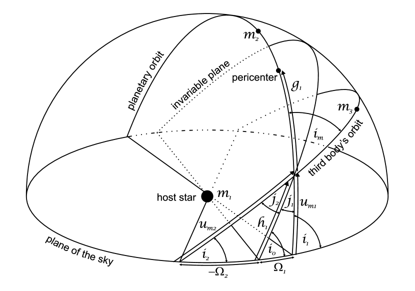
At this point, to avoid any confusion, we emphasize that during our calculations we use different sets of the angular orbital elements. As we are interested in such a phenomenon which primarily depends on the relative positions of the orbiting celestial bodies with respect to the observer, the angular elements (i.e. $u$, $\omega$, $i$, $\Omega$) should be expressed in the “observational” frame of reference having the plane of the sky as the fundamental plane, and $u$, as well as $\omega$ is measured from the intersection of the binary’s orbital plane with that plane, while $\Omega$ is measured along the plane of the sky from an arbitrary origin. On the other hand, the physical variations of the motion of the bodies depend on their relative positions to each other, and consequently, it is more beneficial (and convenient) to express the equations of perturbations of the orbital elements in a different frame of reference, (we shall refer to it as the dynamical frame) which depends on the relative positions of the bodies, independently from any outer observer. The fundamental plane of this latter frame of reference is the invariable plane of the triple system, i.e. the plane perpendicular to the net angular momentum vector of the complete triple system. In this frame of reference the longitude of the ascending node ($h$) gives the arc between the sky and the corresponding intersection of the two orbital planes measured along the invariable plane, while the true longitude ($w$) and the argument of periastron ($g$) is measured from that ascending node, along the respected orbital plane. In order to avoid a further confusion, the relative inclination of the orbits to the invariable plane is denoted by $j$. The meaning and the relation between the different elements can be seen in Fig. 1, and listed also in Appendix A.

Figure 1: The spatial configuration of the system.

2.2 Long period perturbations

From now on we refer to the orbital elements of the inner binary (i.e. the pair formed by either a host star and the inner planet, or two stellar mass objects) by subscript ₁, while those of the wider binary (i.e. the orbit of the third component around the centre of mass of the inner system) by subscript ₂. The differential perturbation equations of the orbital elements are listed in Borkovits et al. (2007). (In that paper, from practical considerations, we did not restrict ourselves to the most usual representation of the perturbation equations, i.e. the Lagrange equations with the perturbing function, rather we used the somewhat more general form, expressing the perturbations with the three orthogonal components of the perturbing force. Nevertheless, as far as only conservative, three-body terms are considered, the two representations are perfectly equivalent.) In order to get the long-period terms of the perturbation equations, the usual method involves averaging the equations for the short-period ($\approx P_{1}$) variables, which is usually the mean anomaly ($l_{1}$) or the true anomaly ($v_{1}$) of the inner binary, but in our special case it is the true longitude $u_{1}$. This means that we get the variation of the orbital elements by averaged for an eclipsing period. Furthermore, in the case of the averaged equations we change the independent variable from $u_{1}$ to (the averaged) $v_{2}$, by the use of

$$\frac{\mathrm{d}u_{1}}{\mathrm{d}v_{2}} \approx \frac{\rho_{2}^{2}}{c_{2}}\frac{c_{1}}{\rho_{1}^{2}}\left(1-\frac{\rho_{1}^{2}}{c_{1}}\dot{\Omega}_{1}\cos i_{1}\right),$$ (6)

from which, after averaging we get:

$$\frac{\mathrm{d}\overline{u_{1}}}{\mathrm{d}\overline{v_{2}}} \approx \frac{\mu_{1}^{1/2}}{a_{1}^{3/2}}\frac{\rho_{2}^{2}}{\sqrt{\mu_{2}a_{2}(1-e_{2}^{2})}}-\frac{\mathrm{d}\overline{\Omega_{1}}}{\mathrm{d}\overline{v_{2}}}\cos i_{1}$$ (7)

$$\approx \frac{P_{2}}{P_{1}}\frac{(1-e_{2}^{2})^{3/2}}{(1+e_{2}\cos v_{2})^{2}}-\frac{\mathrm{d}\Omega_{1}}{\mathrm{d}v_{2}}\cos i_{1}.$$

In the following we omit the overlining. Furthermore, as one can see from Eq. (13) below, the second term in the r.h.s of (7) is of the order $P_{1}/P_{2}$, and consequently can be neglected. So for the long-period perturbations of the orbital elements of the close orbit we get as follows:

$$\frac{\mathrm{d}a_{1}}{\mathrm{d}v_{2}} = 0,$$ (8)

$$\frac{\mathrm{d}e_{1}}{\mathrm{d}v_{2}} = A_{\mathrm{L}}(1-e_{1}^{2})^{1/2}e_{1}(1+e_{2}\cos v_{2})$$ (9)

$$\times\left[\left(1-I^{2}\right)\sin 2g_{1}\right.$$

$$-\frac{1}{2}(1+I)^{2}\sin(2v_{2}+2g_{2}-2g_{1})$$

$$\left.+\frac{1}{2}(1-I)^{2}\sin(2v_{2}+2g_{2}+2g_{1})\right],$$

$$\frac{\mathrm{d}g_{1}}{\mathrm{d}v_{2}} = A_{\mathrm{L}}(1-e_{1}^{2})^{1/2}(1+e_{2}\cos v_{2})$$ (10)

$$\times\left\{\frac{3}{5}\left(I^{2}-\frac{1}{3}\right)\right.$$

$$+\left(1-I^{2}\right)\left[\cos 2g_{1}+\frac{3}{5}\cos(2v_{2}+2g_{2})\right]$$

$$+\frac{1}{2}(1+I)^{2}\cos(2v_{2}+2g_{2}-2g_{1})$$

$$\left.+\frac{1}{2}(1-I)^{2}\cos(2v_{2}+2g_{2}+2g_{1})\right\}$$

$$-\frac{\mathrm{d}h_{1}}{\mathrm{d}v_{2}}\cos{j_{1}},$$

$$\frac{\mathrm{d}h_{1}}{\mathrm{d}v_{2}} = -A_{\mathrm{L}}(1-e_{1}^{2})^{-1/2}\frac{\sin i_{\mathrm{m}}}{\sin{j_{1}}}(1+e_{2}\cos v_{2})$$

$$\times\left[\frac{2}{5}\left(1+\frac{3}{2}e_{1}^{2}\right)I\right.$$

$$-e_{1}^{2}I\cos 2g_{1}$$

$$-\frac{2}{5}\left(1+\frac{3}{2}e_{1}^{2}\right)I\cos(2v_{2}+2g_{2})$$

$$+\frac{1}{2}e_{1}^{2}(1+I)\cos(2v_{2}+2g_{2}-2g_{1})$$

$$\left.-\frac{1}{2}e_{1}^{2}(1-I)\cos(2v_{2}+2g_{2}+2g_{1})\right],$$

$$\frac{\mathrm{d}j_{1}}{\mathrm{d}v_{2}} = A_{\mathrm{L}}(1-e_{1}^{2})^{-1/2}\sin i_{\mathrm{m}}(1+e_{2}\cos v_{2})$$ (11)

$$\times\left[\frac{2}{5}\left(1+\frac{3}{2}e_{1}^{2}\right)\sin(2v_{2}+2g_{2})\right.$$

$$+e_{1}^{2}I\sin 2g_{1}$$

$$-\frac{1}{2}e_{1}^{2}(1+I)\sin(2v_{2}+2g_{2}-2g_{1})$$

$$\left.+\frac{1}{2}e_{1}^{2}(1-I)\sin(2v_{2}+2g_{2}+2g_{1})\right],$$

$$\frac{\mathrm{d}\omega_{1}}{\mathrm{d}v_{2}} = A_{\mathrm{L}}(1-e_{1}^{2})^{1/2}(1+e_{2}\cos v_{2})$$ (12)

$$\times\left\{\frac{3}{5}\left(I^{2}-\frac{1}{3}\right)\right.$$

$$+\left(1-I^{2}\right)\left[\cos 2g_{1}+\frac{3}{5}\cos(2v_{2}+2g_{2})\right]$$

$$+\frac{1}{2}(1+I)^{2}\cos(2v_{2}+2g_{2}-2g_{1})$$

$$\left.+\frac{1}{2}(1-I)^{2}\cos(2v_{2}+2g_{2}+2g_{1})\right\}$$

$$-\frac{\mathrm{d}\Omega_{1}}{\mathrm{d}v_{2}}\cos{i_{1}},$$

$$\frac{\mathrm{d}\Omega_{1}}{\mathrm{d}v_{2}} = A_{\mathrm{L}}(1-e_{1}^{2})^{-1/2}\frac{\sin i_{\mathrm{m}}}{\sin{i_{1}}}(1+e_{2}\cos v_{2})$$ (13)

$$\times\left[\frac{2}{5}\left(1+\frac{3}{2}e_{1}^{2}\right)I\cos(\omega_{1}-g_{1})\right.$$

$$+\frac{1}{5}\left(1+\frac{3}{2}e_{1}^{2}\right)(1-I)\cos(2v_{2}+2g_{2}-\omega_{1}+g_{1})$$

$$-\frac{1}{5}\left(1+\frac{3}{2}e_{1}^{2}\right)(1+I)\cos(2v_{2}+2g_{2}+\omega_{1}-g_{1})$$

$$-e_{1}^{2}I\cos(\omega_{1}+g_{1})$$

$$+\frac{1}{2}e_{1}^{2}(1+I)\cos(2v_{2}+2g_{2}-\omega_{1}-g_{1})$$

$$\left.-\frac{1}{2}e_{1}^{2}(1-I)\cos(2v_{2}+2g_{2}+\omega_{1}+g_{1})\right],$$

$$\frac{\mathrm{d}i_{1}}{\mathrm{d}v_{2}} = A_{\mathrm{L}}(1-e_{1}^{2})^{-1/2}\sin i_{\mathrm{m}}(1+e_{2}\cos v_{2})$$ (14)

$$\times\left[-\frac{2}{5}\left(1+\frac{3}{2}e_{1}^{2}\right)I\sin(\omega_{1}-g_{1})\right.$$

$$+\frac{1}{5}\left(1+\frac{3}{2}e_{1}^{2}\right)(1-I)\sin(2v_{2}+2g_{2}-\omega_{1}+g_{1})$$

$$+\frac{1}{5}\left(1+\frac{3}{2}e_{1}^{2}\right)(1+I)\sin(2v_{2}+2g_{2}+\omega_{1}-g_{1})$$

$$+e^{2}I\sin(\omega_{1}+g_{1})$$

$$-\frac{1}{2}e_{1}^{2}(1+I)\sin(2v_{2}+2g_{2}-\omega_{1}-g_{1})$$

$$\left.+\frac{1}{2}e_{1}^{2}(1-I)\sin(2v_{2}+2g_{2}+\omega_{1}+g_{1})\right],$$

and, finally, the direct term is as follows:

$$\frac{\mathrm{d}\lambda_{1}}{\mathrm{d}v_{2}} = A_{\mathrm{L}}(1-e_{1}^{2})^{1/2}(1+e_{2}\cos v_{2})$$

$$\times\left\{\frac{4}{5}\left(I^{2}-\frac{1}{3}\right)f_{1}(e_{1})\right.$$

$$+\frac{51}{20}\left(1-I^{2}\right)e_{1}^{2}f_{2}(e_{1})\cos 2g_{1}$$

$$+\frac{4}{5}\left(1-I^{2}\right)f_{1}(e_{1})\cos(2v_{2}+2g_{2})$$

$$+\frac{51}{40}(1+I)^{2}e_{1}^{2}f_{2}(e_{1})\cos(2v_{2}+2g_{2}-2g_{1})$$

$$\left.+\frac{51}{40}(1-I)^{2}e_{1}^{2}f_{2}(e_{1})\cos(2v_{2}+2g_{2}+2g_{1})\right\},$$

where

$$A_{\mathrm{L}}=\frac{15}{8}\frac{m_{3}}{m_{123}}\frac{P_{1}}{P_{2}}(1-e_{2}^{2})^{-3/2},$$ (16)

and

$$f_{1}(e) = 1+\frac{25}{8}e^{2}+\frac{15}{8}e^{4}+\frac{95}{64}e^{6},$$ (17)

$$f_{2}(e) = 1+\frac{31}{51}e^{2}+\frac{23}{48}e^{4}.$$ (18)

Furthermore, $i_{\mathrm{m}}$ denotes the mutual inclination of the two orbital planes, while

$$I=\cos i_{\mathrm{m}},$$ (19)

and $m_{123}$ stands for the total mass of the system. Note, formal integration of the first five of the equations above (i.e. those which refer to the orbital elements in the dynamical system, Eqs. [8]-[11]) reproduce the results of Söderhjelm (1982).

Strictly speaking, some of the equations above are valid only in that case when both orbits are non-circular, and the orbital planes are inclined to each other, and/or to the plane of the sky. For example, if the outer orbit is circular, neither $v_{2}$, nor $g_{2}$ has any meaning. Nevertheless, their sum i. e. $v_{2}+g_{2}$ is meaningful as before. Furthermore, although in the case of circular inner orbits the derivative of $g_{1}$ has no meaning, yet the derivative of $e_{1}\cos g_{1}$, $e_{1}\sin g_{1}$ (or $e_{1}\cos\omega_{1}$, $e_{1}\sin\omega_{1}$), i. e. the so-called Lagrangian elements can be calculated correctly. (Note, instead of the “pure” derivatives of $e_{1}$ and $g_{1}$ (or $\omega_{1}$) these latter occur directly in the $O-C$.) Similar redefenitions can be done in the case of coplanarity. So, for practical reasons, and for the sake of clarity, we retain the original formulations even in such cases, when it is formally not valid.

As one can see, there are some terms on the r.h.s. of these equations which do not depend on $v_{2}$. Primarily, these terms give the so-called apse-node time-scale contribution to the variation of the orbital elements and the transit timing variations. Nevertheless, in order to get a correct result for the long-term behaviour of the orbital elements these terms must nevertheless be retained in our long-term formulae. Note, these terms were calculated for tidally distorted triplets in Borkovits et al. (2007). Such formulae (after an omission of the tidal terms) are also valid for the present case in the low mutual inclination (i.e. approx. $I^{2}>\frac{3}{5}$) domain. (Formulae valid for arbitrary mutual inclinations will be presented in a subsequent paper.)

Carrying out the integrations, all the orbital elements on the r.h.s of these equations with the exception of $v_{2}$ are considered as constants. This can be justified for two reasons. First, as one can see, for $P_{2}>>P_{1}$ the amplitudes of the long-period perturbative terms ($A_{\mathrm{L}}$) remain small (which is especially valid for the case where the host star is orbited by two planets, when $m_{3}<<m_{123}$), and second, although the amplitude of the apse-node perturbative terms can reach unity, the period is usually so long ($\sim P_{2}^{2}/P_{1}$, Brown 1936, see e.g.), that its contribution can be safely ignored during one revolution of the outer object. The final result of such an analysis is an analytical form of the transit timing variations, i.e. the long-period $O-C$ diagram. Here we give the result up to the first order in the inner eccentricity, while a more extended result up to the sixth order in the inner eccentricity can be found in appendix B, where we give also the perturbation equations directly for the $e_{1}^{m}\cos{n\omega_{1}}$, $e_{1}^{m}\sin{n\omega_{1}}$ expressions.

$$O-C_{P_{2}} = \frac{P_{1}}{2\pi}A_{\mathrm{L}}(1-e_{1}^{2})^{1/2}\left\{\left(\frac{4}{5}+\frac{5}{2}e_{1}^{2}\mp\frac{6}{5}e_{1}\sin\omega_{1}\right)\right.$$ (20)

$$\times\left[\left(I^{2}-\frac{1}{3}\right){\cal{M}}+\frac{1}{2}\left(1-I^{2}\right){\cal{S}}(2v_{2}+2g_{2})\right]$$

$$+\left[\frac{51}{20}e_{1}^{2}\cos 2g_{1}\mp 2e_{1}\sin(\omega_{1}-2g_{1})\right]$$

$$\times\left[\left(1-I^{2}\right){\cal{M}}+\frac{1}{2}\left(1+I^{2}\right){\cal{S}}(2v_{2}+2g_{2})\right]$$

$$-\left[\frac{51}{20}e_{1}^{2}\sin 2g_{1}\mp 2e_{1}\cos(\omega_{1}-2g_{1})\right]I{\cal{C}}(2v_{2}+2g_{2})$$

$$+\cot i_{1}\sin i_{\mathrm{m}}\left\{-\frac{2}{5}\left(1\mp 2e_{1}\sin\omega_{1}\right)\cos u_{\mathrm{m1}}I\right.$$

$$\times\left[{\cal{M}}-\frac{1}{2}{\cal{S}}(2v_{2}+2g_{2})\right]$$

$$\left.\left.+\frac{1}{5}(1\mp 2e_{1}\sin\omega_{1})\sin u_{\mathrm{m1}}{\cal{C}}(2v_{2}+2g_{2})\right\}\right\}$$

$$-\frac{m_{3}}{m_{123}}\frac{a_{2}\sin i_{2}}{c}\frac{\left(1-e_{2}^{2}\right)\sin(v_{2}+\omega_{2})}{1+e_{2}\cos v_{2}}$$

$$+{\cal{O}}(e_{1}^{2}),$$

where

$${\cal{M}} = \int 1+e_{2}\cos v_{2}\mathrm{d}v_{2}$$

$$= v_{2}-l_{2}+e_{2}\sin v_{2}$$

$$= 3e_{2}\sin v_{2}-\frac{3}{4}e_{2}^{2}\sin 2v_{2}+\frac{1}{3}e_{2}^{3}\sin 3v_{2}+{\cal{O}}(e_{2}^{4})$$

$$= 3e_{2}\left(1-\frac{3}{8}e_{2}^{2}\right)\sin l_{2}+\frac{9}{4}e_{2}^{2}\sin 2l_{2}+\frac{53}{24}e_{2}^{3}\sin 3l_{2}+{\cal{O}}(e_{2}^{4}),$$

and

$${\cal{S}}(2v_{2}+x) \!=\! \sin(2v_{2}+x)+e_{2}\sin(v_{2}+x)+\frac{1}{3}e_{2}\sin(3v_{2}+x)$$

$$\!=\! \left(1-4e_{2}^{2}\right)\sin(2l_{2}+x)$$

$$+e_{2}\left[-\left(1-\frac{13}{8}e_{2}^{2}\right)\sin(l_{2}+x)\right.$$

$$\left.+\frac{7}{3}\left(1-\frac{207}{56}e_{2}^{2}\right)\sin(3l_{2}+x)\right]$$

$$+e_{2}^{2}\left[-\frac{1}{4}\sin{x}+\frac{17}{4}\sin(4l_{2}+x)\right]$$

$$+e_{2}^{3}\left[\frac{1}{24}\sin(l_{2}-x)+\frac{169}{24}\sin(5l_{2}+x)\right]+{\cal{O}}(e_{2}^{4}),$$

$${\cal{C}}(2v_{2}+x) \!=\! \cos(2v_{2}+x)+e_{2}\cos(v_{2}+x)+\frac{1}{3}e_{2}\cos(3v_{2}+x)$$

$$\!=\! \left(1-4e_{2}^{2}\right)\cos(2l_{2}+x)$$

$$+e_{2}\left[-\left(1-\frac{13}{8}e_{2}^{2}\right)\cos(l_{2}+x)\right.$$

$$\left.+\frac{7}{3}\left(1-\frac{207}{56}e_{2}^{2}\right)\cos(3l_{2}+x)\right]$$

$$+e_{2}^{2}\left[-\frac{1}{4}\cos{x}+\frac{17}{4}\cos(4l_{2}+x)\right]$$

$$+e_{2}^{3}\left[-\frac{1}{24}\cos(l_{2}-x)+\frac{169}{24}\cos(5l_{2}+x)\right]+{\cal{O}}(e_{2}^{4}),$$

furthermore,

$$u_{\mathrm{m1}}=\omega_{1}-g_{1},$$ (25)

i.e. $u_{\mathrm{m1}}$ is the angular distance of the intersection of the two orbits from the plane of the sky, or, in other words, the longitude of the (dynamical) ascending node of the inner orbit along the orbital plane, measured from the sky.

Note, the superscripts refer to the exoplanetary transits (primary minima), and the subscripts to the secondary occultations (secondary minima). Furthermore, we assumed the formally second-order $\frac{5}{2}e_{1}^{2}$, and $\frac{51}{20}e_{1}^{2}$ terms, to be first order, as their values exceed $e_{1}$ for medium eccentricities. We included also the pure geometrical light-time contribution in the last row. Here $c$ denotes the speed of light. The minus sign arises because this term reflects the motion of the inner pair around the common centre of mass, whose true longitude differs by $\pi$ from the one of the third component. In Eq. (2.2) the mean anomaly of the outer body ($l_{2}$) appears because of (the constant part of) the difference between the anomalistic $P$ and sideral (eclipsing, or transiting) $P_{\mathrm{s}}$ period included into the first term in the r.h.s. of Eq. (LABEL:eq:apsisexp).

3 Discussion of the results

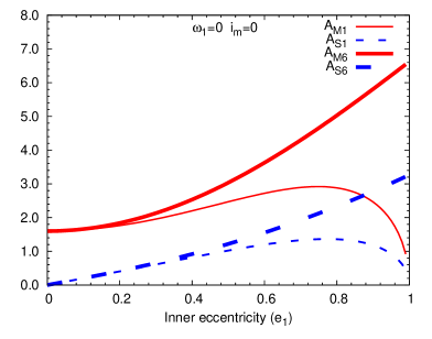
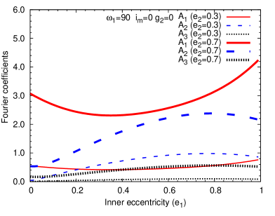
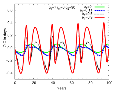
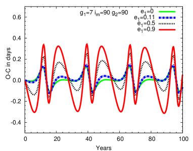
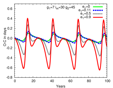
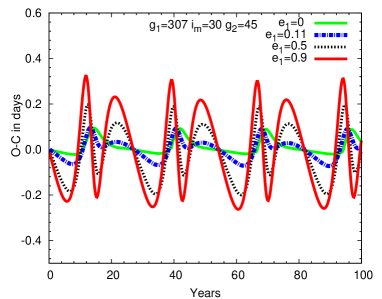
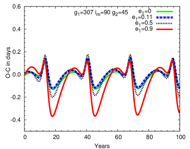
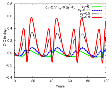
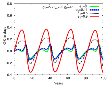
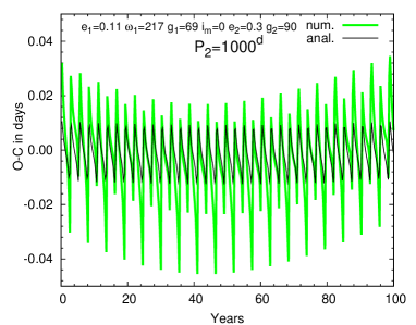
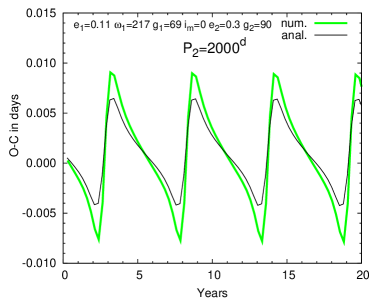
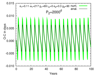
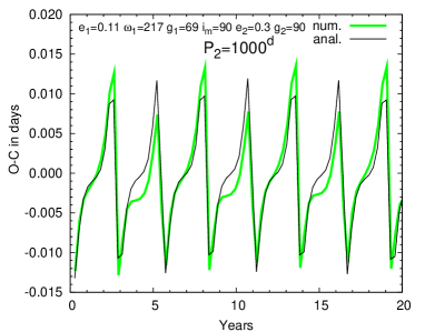
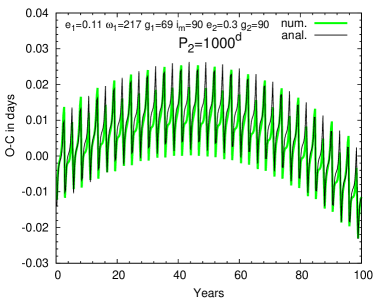
As one can easily see, the result for a circular inner orbit (i.e. $e_{1}=0$) is identical with the formula (46) of Borkovits et al. (2003). Consequently, the discussion given in Sect. 4 of that paper is also valid. Nevertheless, as one can see in Figs. 2, 3, a significant inner eccentricity produces notably higher amplitudes, and consequently, is easier to detect. Furthermore, some other attributes of the transit timing variations also change drastically. For example, in contrast to the previously studied coplanar ($I=\pm 1$), circular inner orbit ($e_{1}=0$) case, (Borkovits et al. 2003; Agol et al. 2005), as long as the inner orbit is eccentric, the dynamical term does not disappear even if the outer orbit is circular ($e_{2}=0$). A further important feature for eccentric inner orbit, in that the amplitude, the phase and the shape of the $O-C$ variations cease to be depend simply on the physical (i.e. relative) positions of the celestial bodies, but also on the orientation of the orbit with respect to the observer. These latter elements (i. e. $e_{1}\sin\omega_{1}$, $e_{1}\cos\omega_{1}$ and their combinations) can also be determined from radial velocity measurements, as well as from the shape of the transit light-curves, and, in the case of the possible detection of the occultation, or (in the case of eclipsing binaries), of the secondary minimum, from the time delay between the two different eclipsing events. So, while the relative, i.e. physical angular parameters (i.e. periastron distances from the intersection of the two orbits, $g_{1}$, $g_{2}$, and mutual inclination $i_{\mathrm{m}}$) cannot be aquired from other, generally used methods (e.g. light-curve, or simple radial velocity curve analysis), these observational geometrical parameters could be determined from other sources of information, and then simply can be built into such a fitting algorithm, which was described in Borkovits et al. (2003), or could be included into such procedures which were presented by Pál (2010).

In the following, as we are mainly interested in transiting systems, where $i_{1}\approx 90\degr$ (which is especially true for relatively longer period, i.e. distant transiting exoplanets), we omit terms multiplied by $\cot i_{1}$, i.e. terms arising from nodal motion.

In Borkovits et al. (2003) we considered only triple stellar systems, where the three masses were usually nearly equal, and the inner period was of the order of a few days. In such cases light-time term dominates. The amplitude of the light-time effect is simply

$$A_{\mathrm{LITE}} = \frac{m_{3}}{m_{123}}\frac{a_{2}\sin i_{2}}{c}\left(1-e_{2}^{2}\cos^{2}\omega_{2}\right)^{1/2}$$ (26)

$$= \frac{m_{3}}{m_{123}}\left(\frac{Gm_{123}}{4\pi^{2}}\right)^{1/3}\frac{\sin i_{2}}{c}P_{2}^{2/3}\left(1-e_{2}^{2}\cos^{2}\omega_{2}\right)^{1/2}$$

$$\approx 1.1\times 10^{-4}\frac{m_{3}}{m_{123}^{2/3}}\sin i_{2}P_{2}^{2/3}\left(1-e_{2}^{2}\cos^{2}\omega_{2}\right)^{1/2},$$

where masses should be expressed in solar units, and $P_{2}$ in days.

The amplitude of the dynamically forced $O-C$, and consequently, the detectability limit of such perturbations depends on almost the all dynamical as well as geometrical variables. So, we can give only some limits on the detectability limit. Nevertheless, for an easier, and somewhat general study, we separate the physical and geometrical variables from each other, and furthermore, we separate also the elements of the inner orbit from those of the outer perturber (with the exception of the mutual inclination). In order to do this, we introduce the following quantities, all of which depend on eccentricity ($e_{1}$), the two types of periastron arguments ($g_{1}$, $\omega_{1}$), and mutual inclination ($i_{\mathrm{m}}$), via its cosine:

$$\alpha = \left\{\frac{2}{5}+\frac{5}{4}e_{1}^{2}\left(1+\cos 2g_{1}\right)\mp e_{1}\left[\frac{3}{5}\sin\omega_{1}+\sin(\omega_{1}-2g_{1})\right]\right.$$ (27)

$$-I^{2}\left\{\frac{2}{5}+\frac{5}{4}e_{1}^{2}\left(1-\cos 2g_{1}\right)\right.$$

$$\left.\left.\mp e_{1}\left[\frac{3}{5}\sin\omega_{1}-\sin(\omega_{1}-2g_{1})\right]\right\}\right\}\left(1-e_{1}^{2}\right)^{1/2},$$

$$\beta = -\left(1-e_{1}^{2}\right)^{1/2}2I\left[\frac{5}{4}e_{1}^{2}\sin 2g_{1}\mp e_{1}\cos(\omega_{1}-2g_{1})\right],$$ (28)

$$\gamma = \left\{\!-\frac{4}{15}\!+\!\frac{5}{2}e_{1}^{2}\left(\cos 2g_{1}-\frac{1}{3}\right)\mp 2e_{1}\left[\sin(\omega_{1}-2g_{1})-\!\frac{1}{5}\sin\omega_{1}\!\right]\right.$$ (29)

$$+I^{2}\left\{\frac{4}{5}+\frac{5}{2}e_{1}^{2}\left(1-\cos 2g_{1}\right)\right.$$

$$\left.\left.\mp 2e_{1}\left[\frac{3}{5}\sin\omega_{1}-\sin(\omega_{1}-2g_{1})\right]\right\}\right\}\left(1-e_{1}^{2}\right)^{1/2}.$$

Then

$$O-C_{\mathrm{dyn}}\approx\frac{P_{1}}{2\pi}A_{\mathrm{L}}\left[\gamma{\cal{M}}+\!\!\sqrt{\alpha^{2}+\beta^{2}}{\cal{S}}(2v_{2}+\phi)\right],$$ (30)

where

$$\phi=2g_{2}+\arctan\frac{\beta}{\alpha}$$ (31)

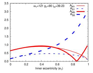
or, in trigonometric form

$$O-C_{\mathrm{dyn}}\approx\frac{P_{1}}{2\pi}A^{*}_{\mathrm{L}}\sum_{n}A_{n}\sin(nv_{2}+\phi_{n}),$$ (32)

where (up to third order in $e_{2}$)

$$A_{1} = \left(1-e_{2}^{2}\right)^{-3/2}e_{2}\sqrt{A_{\cal{S}}^{2}+A_{\cal{M}}^{2}+2A_{\cal{S}}A_{\cal{M}}\cos\phi},$$ (33)

$$A_{2} = \left(1-e_{2}^{2}\right)^{-3/2}\sqrt{A_{\cal{S}}^{2}+\frac{1}{16}e_{2}^{4}A_{\cal{M}}^{2}+\frac{1}{2}e_{2}^{2}A_{\cal{S}}A_{\cal{M}}\cos\phi},$$ (34)

$$A_{3} = \left(1-e_{2}^{2}\right)^{-3/2}\frac{1}{3}e_{2}\sqrt{A_{\cal{S}}^{2}+\frac{1}{9}e_{2}^{4}A_{\cal{M}}^{2}+\frac{2}{3}e_{2}^{2}A_{\cal{S}}A_{\cal{M}}\cos\phi},$$ (35)

$$\phi_{1} = \arctan\frac{\sin\phi}{\cos\phi+\frac{A_{\cal{M}}}{A_{\cal{S}}}},$$ (36)

$$\phi_{2} = \arctan\frac{\sin\phi}{\cos\phi+\frac{1}{4}e_{2}^{2}\frac{A_{\cal{M}}}{A_{\cal{S}}}},$$ (37)

$$\phi_{3} = \arctan\frac{\sin\phi}{\cos\phi+\frac{1}{9}e_{2}^{2}\frac{A_{\cal{M}}}{A_{\cal{S}}}},$$ (38)

and

$$A_{\cal{S}} = \sqrt{\alpha^{2}+\beta^{2}},$$ (39)

$$A_{\cal{M}} = 3\gamma,$$ (40)

and, furthermore,

$$A^{*}_{\mathrm{L}}=A_{\mathrm{L}}\left(1-e_{2}^{2}\right)^{3/2}.$$ (41)

Note, for a circular outer orbit ($e_{2}=0$)

$$A_{1}=A_{3} = 0,$$ (42)

$$A_{2} = A_{\cal{S}}.$$ (43)

As one can see, both sets of amplitudes, i.e. $A_{{\cal{M}},{\cal{S}}}$ and $A_{1,2,3}$ are independent of the real physical parameters of the current exoplanetary system. Furthermore, the dependence from the elements of the outer orbit (i.e. $e_{2}$, $g_{2}$) appear only in the $A_{1,2,3}$ Fourier amplitudes. The masses (or more accurately mass ratios), and the periods and period ratios (and indirectly the physical size of the system) occur only as a scaling parameter. In this way, the following general statements are valid for every hierarchical triple systems (as far as the initial model assumptions are valid). In order to get the real, i.e. physical values for the $O-C$ amplitudes in a given system, one must multiply the general system-independent, dimensionless amplitudes with the system specific number $\frac{15}{16\pi}\frac{P_{1}^{2}}{P_{2}}\frac{m_{3}}{m_{1}+m_{2}+m_{3}}$.

Considering first the (nearly) coplanar case, i.e. when $I\approx\pm 1$, then the (half-)amplitude of the two sinusoidals becomes:

$$e_{2}A_{{\cal{M}}0} \approx \frac{8}{5}\left(1-e_{1}^{2}\right)^{1/2}\left(1+\frac{25}{8}e_{1}^{2}\mp\frac{3}{2}e_{1}\sin\omega_{1}\right)e_{2},$$ (44)

$$A_{{\cal{S}}0} \approx 2\left(1-e_{1}^{2}\right)^{1/2}e_{1}\sqrt{1\mp\frac{5}{2}e_{1}\sin\omega_{1}+\frac{25}{16}e_{1}^{2}}.$$ (45)

This illustrates the above-mentioned fundamental differences to the previously-studied coplanar, $e_{1}=0$ case (Borkovits et al. 2003; Agol et al. 2005), as according to our new result for eccentric inner orbits, the dynamical term does not disappear even if the outer orbit is circular ($e_{2}=0$). Furthermore, the amplitudes strongly depend on the orientation of the orbital axis with respect to the observer. When the apsidal line coincides (more or less) with the line of sight (i.e. $\omega_{1}=\pm 90\degr$) there can be very significant differences both in the shape and amplitude of the primary (transit) and secondary (occultation) $O-C$ curves. However, when the apsidal line lies nearly in the sky, then these differences disappear. A further interesting feature of the $\omega_{1}=\pm 90\degr$ configuration, is that for eclipse events which occur around apastron there is a full square under the square-root sign in the ${\cal{S}}$-term, with the root of $e_{1}=0.8$, which means that in this situation this term would disappear. Nevertheless, for such a high eccentricity the first order approximation is far from being valid, as is illustrated in Fig. 2.

For highly inclined ($I\approx 0$) orbits the (half-)amplitudes are as follows:

$$e_{2}A_{{\cal{M}}90} \approx \frac{4}{5}\left(1-e_{1}^{2}\right)^{1/2}\left\{-1-\frac{25}{8}e_{1}^{2}\left(1-3\cos 2g_{1}\right)\right.$$ (46)

$$\left.\pm\frac{3}{2}e_{1}\left[\sin\omega_{1}-5\sin(\omega_{1}-2g_{1})\right]\right\}e_{2},$$

$$A_{{\cal{S}}90} \approx \frac{2}{5}\left(1-e_{1}^{2}\right)^{1/2}\left\{1+\frac{25}{8}e_{1}^{2}\left(1+\cos 2g_{1}\right)\right.$$ (47)

$$\left.\mp\frac{3}{2}e_{1}\left[\sin\omega_{1}+\frac{5}{3}\sin(\omega_{1}-2g_{1})\right]\right\},$$

furthermore, the phase of the ${\cal{S}}$-term is simply

$$\phi=2g_{2}.$$ (48)

In this case a further parameter, namely, the periastron distance of the inner planet from the intersection of the two orbital planes ($g_{1}$) also plays an important role.

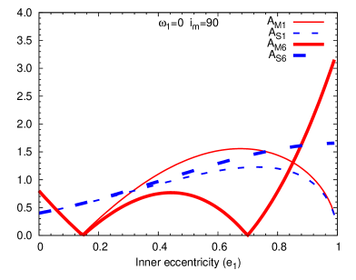
Finally we also mention a very specific case, namely for the maximum eccentricity phase of the Kozai mechanism driven $e$-cycles. During this phase, $\cos 2g_{1}$ takes one definite value, namely $\cos 2g_{1}=-1$. Furthermore, the mutual inclination of the two orbits here reaches its minimum. The actual value depends on both the maximum mutual inclination $i_{\mathrm{m}}$, or more strictly, on $j_{1}$, and the minimal inner eccentricity $e_{1}$. Nevertheless, in the case of an initially almost circular inner orbit, the minimum mutual inclination is almost independent of its maximum value, and takes $j_{1}(\approx i_{\mathrm{m}})\approx 39\aas@@fstack{\circ}23$ (or its retrograde counterpart, $j_{1}(\approx i_{\mathrm{m}})\approx 140\aas@@fstack{\circ}77$), i.e. $I^{2}=3/5$. For this scenario:

$$e_{2}A_{{\cal{M}}\mathrm{Kozai},90} \approx \frac{16}{25}\left(1-e_{1}^{2}\right)^{1/2}\left(1-\frac{25}{16}e_{1}^{2}\pm\frac{9}{4}e_{1}\sin\omega_{1}\right)e_{2},$$ (49)

$$\alpha_{\mathrm{Kozai},90} = \left(1-e_{1}^{2}\right)^{1/2}\left(\frac{4}{25}-\frac{5}{3}e_{1}^{2}\pm\frac{34}{25}e_{1}\sin\omega_{1}\right),$$

$$\beta_{\mathrm{Kozai},90} = \mp\left(1-e_{1}^{2}\right)^{1/2}\frac{2}{5}\sqrt{15}e_{1}\cos\omega_{1}.$$ (50)

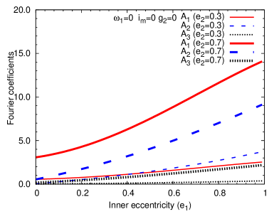
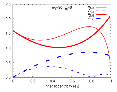
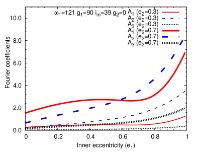
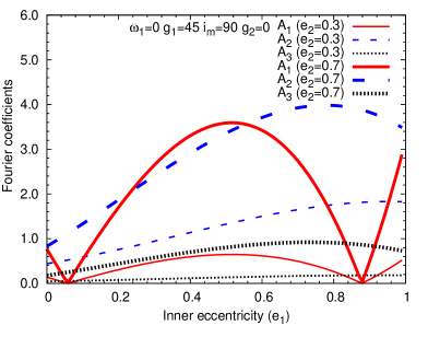
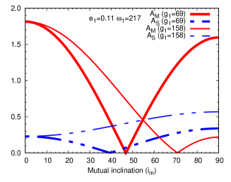
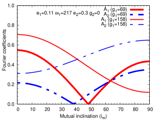
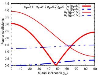
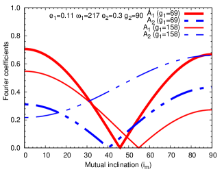
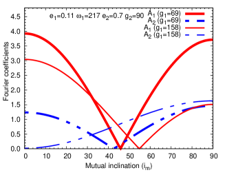
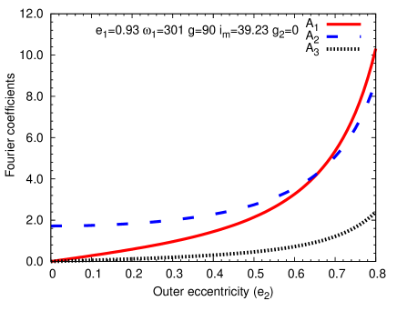
In order to get a better overview of the parameter dependence of the formulae above, we investigate the $A_{{\cal{M}},{\cal{S}}}$, as well as the $A_{1,2,3}$ amplitudes graphically. Due to the complex dependence of these amplitudes on many parameters, it is difficult to give general statements. Therefore we investigate only the dependence of the amplitudes on the inner eccentricity, while the effects of other parameters will be considered in Sect. 4 for specific systems, where some of the parameters can be fixed.

Fig. 2 shows the inner eccentricity ($e_{1}$) dependence of the amplitudes for some specific values of the other parameters. In general, one sees that the $e_{1}$ increase with amplitude, but this growth usually remains within one order of magnitude. So, although the shapes of the individual $O-C$ curves may differ significantly, the net amplitudes vary over a narrow range. The graphs also suggest another, perhaps suprising fact, that the amplitude of $O-C_{\mathrm{P2dyn}}$ depends only weakly on the mutual inclination ($i_{\mathrm{m}}$). This is especially valid for medium inner eccentricities, since in this case, at least for the cases shown in Fig. 2, all $A_{{\cal{M}},{\cal{S}}}$ amplitudes have similar values. Moreover, the numerically generated sample $O-C$ curves of Fig. 3, also suggest such a conclusion. Nevertheless, there are several exceptions. Some particular configurations some of the amplitudes, or even both of them (and consequently, the corresponding terms) can disappear. Such a situation will be discussed in Sect. 4.1. We will return to this question in detail in Sect. 4, where the dependence of the amplitudes on other parameters will be also studied for the systems of CoRoT-9b and HD 80606b.

Figure 2: Left panels: The inner eccentricity ($e_{1}$) dependence of $A_{\cal{M}}$, $A_{\cal{S}}$ amplitudes of ${\cal{M}}$, ${\cal{S}}$ functions of long-period dynamical part of $O-C$ for specific values of some parameters. Note, to compare the ${\cal{M}}$ and ${\cal{S}}$ terms, the former should be multiplied by $e_{2}$. The thin lines (indexed by ’1’) refer to the first order approximation, while the thick ones (index ’6’) to the sixth one. Right panels: The corresponding $A_{1,2,3}$ amplitudes of the trigonometric representation (Eq. 32) of the $O-C$ for two different outer eccentricities ($e_{2}=0.3$ and $e_{2}=0.7$) ($g_{2}$ was set to 0°).

Figure 3: Transit timing variatons caused by a hypothetical $P_{2}=10\,000$ day-period $m_{3}=1M_{\mathrm{\sun}}$ mass, moderately eccentric $e_{2}=0.3$ third companion for CoRoT-9b, at different initial orbital elements, for four different initial inner eccentricities ($e_{1}=0$, 0.11, 0.5, 0.9). The various initial elements of each panel are as follows. Panel $(a)$: $g_{1}=7\degr$, $g_{2}=90\degr$, $i_{\mathrm{m}}=0\degr$; $(b)$: The same, but for $i_{\mathrm{m}}=90\degr$; $(c)$: $g_{1}=7\degr$, $g_{2}=45\degr$, $i_{\mathrm{m}}=30\degr$; $(d)$: $g_{1}=337\degr$, $g_{2}=45\degr$, $i_{\mathrm{m}}=60\degr$; $(e)$: $g_{1}=307\degr$, $g_{2}=45\degr$, $i_{\mathrm{m}}=30\degr$; $(f)$: same as previous, but for $i_{\mathrm{m}}=90\degr$. $(g)$: $g_{1}=277\degr$, $g_{2}=45\degr$, $i_{\mathrm{m}}=0\degr$; $(h)$: same as previous, but for $i_{\mathrm{m}}=90\degr$. (For better comparison the curves are corrected for the different average transit periods, and zero point shifts.)

Returning now to the LITE amplitude, and comparing it with the dynamical case, an increment of $P_{2}$ (keeping $P_{1}$ constant) results in an increment of $A_{\mathrm{LITE}}/A_{\mathrm{P2-dyn}}$ by $P_{2}^{5/3}$. Consequently, for more distant systems the pure geometrical effect tends to exceed the dynamical one, as is the case in all but one ($λ$ Tau, Söderhjelm 1975, see e. g.) of the known hierarchical eclipsing triple stellar systems. Nevertheless, as we will illustrate in this paper (see Fig. 5), we have a good chance of finding the opposite situation in some of the recently discovered transiting exoplanetary systems. We can make the following crude estimation. Consider a system with a solar-like host star, and two approximately Jupiter-mass companions) ($m_{123}\approx m_{1}=1\mathrm{M}_{\odot}$, $m_{2}=m_{3}=10^{-3}\mathrm{M}_{\odot}$) choosing $A=10^{-3}$ day for the case of a certain detection, then the LITE term for the most ideal case gives $P_{2}\geq 10^{6}\mathrm{d}\approx 2\,700\mathrm{y}$. Alternatively, setting $m_{3}=10^{-2}\mathrm{M}_{\odot}$, and allowing $A=10^{-4}$ for detection limit, the result is $P_{2}\geq 10^{3}\mathrm{d}\approx 2.7\mathrm{y}$. Similarly, for two Jupiter-mass planet, in the coplanar case, for small $e_{1}$, the $A=10^{-3}$ day limit gives

$$P_{2}\leq 2\times 10^{3}m_{3}e_{2}\left(1-e_{2}^{2}\right)^{-3/2}P_{1}^{2}$$ (51)

condition for the detectability of a third companion by its long-term dynamical perturbations. For the perpendicular case the same limit is

$$P_{2}\leq\frac{1}{2}\times 10^{3}m_{3}\left(1-e_{2}^{2}\right)^{-3/2}\left(1+\frac{2}{3}e_{2}\right)P_{1}^{2}.$$ (52)

We note that for $m_{3}<<m_{1}$ the above equations are linear for $m_{3}$, so it is very easy to give the limiting period $P_{2}$ in the function of $m_{3}$. Nevertheless, we emphasize again that there are so many terms with different periodicity and phase, that these equations give only a very crude, first estimation. For $P_{1}=$1, 10, 100 days, (at zero outer eccentricity) gives $P_{2}\leq$0.5, 50, $5\,000$ days, respectively,

These results refer to the total amplitude of the $O-C$ curve, i.e. the variation of the transit times during a complete revolution of the distant companion, which can take as long as several years or decades. Naturally, the perturbations in the transit times could be observed within a much shorter period, from the variation of the interval between consecutive minima. This estimation can be calculated e.g from Eq. (30), or even directly from Eq. (LABEL:Eq:dlambda1dv2). According to the meaning of the $O-C$ curve, the transiting or eclipsing period ($\overline{P}$) between two consecutive (let us assume the $n$-th and $n+1$-th) minima is

$$\overline{P}_{n}=t_{n+1}-t_{n} = \left(O-C\right)(t_{n+1})-\left(O-C\right)(t_{n})$$ (53)

$$\approx P_{\mathrm{s}}+\frac{P_{1}}{2\pi}A_{\mathrm{L}}\left(1-e_{1}^{2}\right)^{1/2}\Delta v_{2n}\left(1+e_{2}\cos v_{2n}\right)$$

$$\times\left[\gamma+2\sqrt{\alpha^{2}+\beta^{2}}\cos(2v_{2n}+\phi)\right],$$

where up to third order in $e_{2}$

$$\Delta v_{2} \approx \Delta l_{2}\left(1+2e_{2}^{2}+2e_{2}\cos v_{2}+\frac{1}{2}e_{2}^{2}\cos 2v_{2}+3e_{2}^{3}\cos 3v_{2}\right)$$ (54)

$$\approx 2\pi\frac{\overline{P}}{P_{2}}(1+\delta v_{2})$$

$$\approx 2\pi\frac{P_{1}}{P_{2}}(1+\delta v_{2}),$$

i. e. we approximated the variation of the mean anomaly of the outer companion ($l_{2}$) by the constant value of

$$\Delta l_{2}\approx 2\pi\frac{P_{1}}{P_{2}}.$$ (55)

(Here, and in the following text we neglect the pure geometrical LITE contribution.) Then the variation of the length of the consecutive transiting periods becomes

$$\Delta\overline{P} \approx -\frac{15}{4}\pi\frac{m_{3}}{m_{123}}\frac{P_{1}^{4}}{P_{2}^{3}}\frac{\left(1-e_{1}^{2}\right)^{1/2}}{\left(1-e_{2}^{2}\right)^{3/2}}$$ (56)

$$\times\left\{\gamma\left[3e_{2}\left(1+\frac{9}{2}e_{2}^{2}\right)\sin v_{2}-6e_{2}^{2}\sin 2v_{2}-\frac{9}{2}e_{2}^{3}\sin 3v_{2}\right]\right.$$

$$+2\sqrt{\alpha^{2}+\beta^{2}}\left[2\left(1+8e_{2}^{2}\right)\sin(2v_{2}+\phi)\right.$$

$$+\frac{7}{2}e_{2}\left(1+\frac{9}{2}e_{2}^{2}\right)\sin(v_{2}+\phi)$$

$$+\frac{13}{2}e_{2}\left(1+\frac{9}{2}e_{2}^{2}\right)\sin(3v_{2}+\phi)$$

$$\left.\left.+\frac{1}{4}e_{2}^{3}\sin(-v+\phi)+\frac{19}{4}e_{2}^{3}\sin(5v_{2}+\phi)\right]\right\}.$$

Comparing (the amplitude of) this result with Eqs. (1,2) of Holman & Murray (2005), one can see that the power of the period ratio differs. (Furthermore, in the original paper $\pi$ stands at the same place, i.e. in the numerator (as above) but later, in Holman 2010 this was declared as an error, and it was put into the denominator.) There is a principal difference in the background. Holman & Murray (2005) state that they “estimate the variation in transit intervals between successive transits”, but what they really calculate is the departure of a transiting period (i.e. the interval between two successive transits) from a constant mean value. This quantity was estimated in our Eq. (53). In other words, the Lagrangian perturbation equations gives the instantaneous period of the perturbed system. So, its integration gives the time left between two consecutive minima. The first derivative of the perturbation equation gives the instantaneous period variation, and so the variation of the length of two consecutive transiting period can be deduced by integrating the latter. As a consequence, the best possibility for the detection of the transit timing variation, and so, for the presence of some perturber occurs when the absolute value of the second derivative of the $O-C$ diagram, or practically Eq. (56) (the period variation during a revolution) is maximum. We will illustrate this statement in the next Section for specific systems.

4 Case studies

4.1 CoRoT-9b

Figure 4: Left panels: The mutual inclination ($i_{\mathrm{m}}$) dependence of $A_{\cal{M}}$, $A_{\cal{S}}$ amplitudes of ${\cal{M}}$, ${\cal{S}}$ functions of the long-period dynamical component of $O-C$ for CoRoT-9b, for $g_{1}=69$°and $g_{1}=158$°. For other $g_{1}$ values the corresponding curves run within the area limited by these lines. (The two left panels are identical.) Middle and right panels: The corresponding $A_{1,2}$ amplitudes of the trigonometric representation (Eq. 32) of the $O-C$ for two different outer eccentricities $e_{2}=0.3$ (middle) and $e_{2}=0.7$ (right); and outer dynamical (relative) argument of pericentrum arguments $g_{2}=0$°(up) and $g_{2}=90$°(down). For the sake of clarity, we did not plot the small $A_{3}$ coefficients. (Note, for $e_{2}=0.0$ the $A_{\cal{S}}$ amplitudes of the two identical left panels are equal to $A_{2}$, while $A_{1}=A_{3}=0$.)

CoRoT-9b is a transiting giant planet which revolves around its host star approximately at the distance of Mercury (Deeg et al. 2010). Consequently, tidal forces (including the possible rotational oblateness) can safely be neglected in this system. Furthermore, due to the relatively large absolute separation of the planet from its star, we can expect a large amplitude signal from the perturbations of a hypothetical, distant (but not too distant) further companion. To illustrate this possibility, and, furthermore, to check our formulae, we both calculated and plotted the amplitudes with the measured parameters of this specific system, and carried out short-term numeric integrations for comparison. The physical, and some of the orbital elements of CoRoT-9b were taken from Deeg et al. (2010). These data are listed in Table 1. (Note, we added $180$°to the $\omega_{1}$ published in that paper, as the spectroscopic $\omega_{1}$ refers to the orbit of the host star around the common centre of mass of the star-planet double system, and consequently, differ by $180$°from the observational argument of periastron of the relative orbit of the transiting planet around its host star.) In the case of the numerical integrations, the inner planets were started from periastron, while the outer one from its apastron.

Fixing the observationally aquired data, $A_{{\cal{M}},{\cal{S}}}$ depend only on two parameters, namely $g_{1}$ and $i_{\mathrm{m}}$. In the left panels of Fig. 4 we plotted the $i_{\mathrm{m}}$ versus $A_{{\cal{M}},{\cal{S}}}$ graphs for $g_{1}=69$°and $g_{1}=158$°. We found that the amplitudes reach their extrema around these periastron arguments, i.e. for other $g_{1}$ values results occur within the areas limited by these lines. In the middle and right panels the effect of the two further free parameters, i.e. outer eccentricity ($e_{2}$), and dynamical (relative) argument of periastron ($g_{2}$) were also considered. The middle panels show $A_{1,2}$ for $e_{2}=0.3$, the right panels for $e_{2}=0.7$, for both $g_{2}=0$°(upper panels), and $g_{2}=90$°(bottom panels). (Note, that $A_{\cal{S}}$, plotted in the left panel is identical to $A_{2}$ for $e_{2}=0$, in which case $A_{1,3}=0$.)

These figures clearly show again that the amplitudes, and consequently, the actual full amplitude of the dynamical $O-C$ curve remains within one order of magnitude over a wide range of orbital parameters. This once more verifies the very crude estimations given by Eqs. (51,52). As a consequence, for a given system we can estimate very easily the expected amplitude of the $O-C$ variations induced by a further companion. For a planet-mass third body, the

$$A_{\mathrm{dyn}}\approx\frac{1}{2\pi}\frac{m_{3}}{P_{2}}\frac{P_{1}^{2}}{m_{\mathrm{host-star}}}$$ (57)

gives a likely estimation at least in magnitude. For example, for CoRoT-9b

$${\cal{A}}=\frac{1}{2\pi}\frac{P_{1}^{2}}{m_{\mathrm{host-star}}} \approx 1459\mathrm{d}^{2}\mathrm{M}_{\mathrm{\sun}}^{-1}$$ (58)

$$\approx 1.39\mathrm{d}^{2}\mathrm{M}_{\mathrm{J}}^{-1},$$

i.e. a Jupiter-mass additional planet could produce $0\aas@@fstack{d}001$ half-amplitude already from the distance of the Mars. (Of course, if $e_{1}$ and $\omega_{1}$ are known, a more precise estimation can be provided easily using the formulae of the present paper.)

Nevertheless, while the net amplitudes usually vary in a narrow range, the dominances of the two main terms (with period $P_{2}$ and $\frac{1}{2}P_{2}$) can alternate and, although it is not shown, their relative phase can also vary so, the shape of the actual curves may show great diversity, as is illustrated e.g. in Figs. 3, 5. Furthermore, for specific values of the parameters, one or the other amplitudes might disappear. At CoRoT-9b particularly interesting is the $g_{1}=69$°$i_{\mathrm{m}}\sim 45$°configuration since in this case both $A_{\cal{M}}$ and $A_{\cal{S}}$ disappear very close to each other. This means that for specific $e_{2}$, $g_{2}$ values the dynamical $O-C$ almost disappears. This possibility warns us of the fact, that from the absence of $TTV$ in a given system one cannot automatically exclude the presence of a further planet (which should be observed according to its parameters).

Figure 5: Sample of transit timing variations caused by a hypothetical $P_{2}=10\,000$ day-period $m_{3}=0.005M_{\mathrm{\sun}}(\approx 5M_{\mathrm{J}})$ mass third companion for CoRoT-9b at four different initial mutual inclinations ($i_{\mathrm{m}}=0$°, 40°, 46°, 90°, from up to down), and three different initial outer eccentricities ($e_{2}=0$, 0.3, 0.7, from left to right). The dynamical (relative) arguments of periastrons are set to $g_{1}=69$°, $g_{2}=90$°. The curves show the sum of the geometrical LITE, and the dynamical terms obtained both from numeric integrations, and analytic calculations up to sixth order in $e_{1}$. The pure LITE contributions are also plotted separately. Note that the vertical scale of the individual columns (i.e. different $e_{2}$-s) are different.

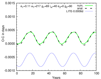
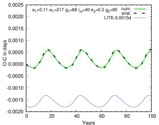
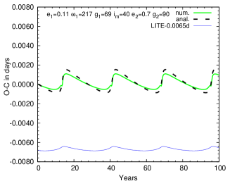
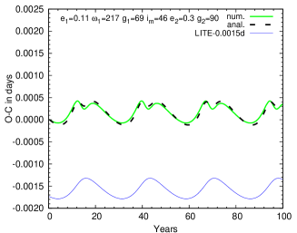
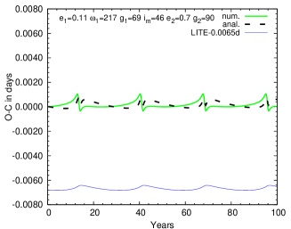
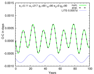
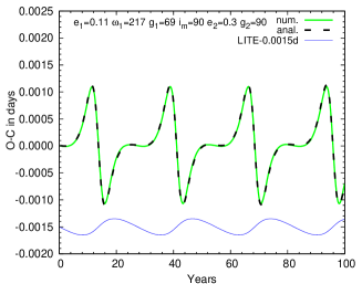
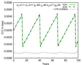
This can be seen clearly in Fig. 5, where we plotted the corresponding $O-C$ curves for coplanar, perpendicular, and the above mentioned interesting $i_{\mathrm{m}}=40$°and 46°configurations. In this latter figure we plotted $O-C$ curves obtained from both numerical integrations of the three-body motions, and analytical calculations with our sixth order formula. (Note, according to Fig. 2, for the small inner eccentricity of CoRoT-9b ($e_{1}=0.11$), the first order approximation would have given practically the same results.) Comparing the analytical and the numerical curves, the best similarity can be seen in the perpendicular case (last row). In the coplanar case some minor discrepancies can be observed both in the shape and amplitude, while the discrepancies are more expressed in the particular $i_{\mathrm{m}}=46$°case, where for large outer eccentricity (right panel in the third row) our solution fails. (Nevertheless, the total amplitude of the analytical curve is similar to the numerical one in this case, too.) Although a thorough analysis of the sources of the discrepancies is beyond the scope of this paper, we suppose that in these situations the discrepancies come from the higher order perturbative terms. As was shown e.g. by Söderhjelm (1982); Ford et al. (2000) the higher order contributions are the most significant for $e_{1}\sim 0$, $i_{\mathrm{m}}=(0,1)\times 180$°. Although the above authors considered only the secular, or apse-node term perturbations, the same might be the case for the long-period ones. This might explain the better correspondance in the perpendicular configuration than in the coplanar one. We suppose some similar reason in the $i_{\mathrm{m}}=46$°case. As in this situation the first order contributions almost disappear, whereas the small higher order terms can also be more significant. Furthermore, numeric integrations in this latter case show a disappearence of the identity between the $g_{1}$, $g_{1}+180$°initial conditions, which also suggests a significance of the higher order terms as in this case we can expect the appearance of trigonometric functions with $g_{1}$ and $3g_{1}$ in their arguments.

Figure 6: The first and the second 8 years of $O-C$-s plotted in the first and the last rows of Fig. 5. The periods of the individual curves were set equal to the respective initial transiting periods.

As expected, the highly eccentric-distant-companion scenario produces the largest amplitude TTV, at least when a complete revolution is considered. Nevertheless, on a shorter time-scale, the length of the observing window necessary for the detection depends highly on the phase of the curve. To illustrate this, in Fig. 6 we plotted the first, and second 8 years of the three primary transit $O-C$ curves for both the coplanar, and the perpendicular cases, shown in the first and last rows of Fig. 5. The transiting periods for each curve were calculated in the usual, observational manner, i.e. the time interval between the first (some) transits were used. According to Fig. 6, in the present situation, in the first 8 years (i.e. which begins at the apastron of the outer planet) it would be unlikely to detect the perturbations in the largest (total) amplitude $e_{2}=0.7$ cases, as well as in the coplanar $e_{2}=0.3$ case. The most certain detection would be possible in the two smallest amplitude circular $e_{2}=0$ configurations. Nevertheless, if the observations starts at those phases plotted on the right panels (8-16 years), the pictures completely differ. In this latter interval, the circular cases produce the smallest curvature $O-C$-s, and the discrepancy from the linear trend reaches $0\aas@@fstack{d}001$ days (which can be considered as a limit for certain detection) occuring towards the end of the interval. On the other hand, in the case of the highly eccentric configurations, the ’moment of truth’ comes after some years. Nevertheless, we have to stress, that although we plotted the $O-C$ curves with continuous lines, in reality they would contain only 3-4 points during the phase of the seemingly abrupt jump, is a further complicating factor with regards to ’certain’ detection.

Figure 7: Checking the validity of hierarchical approximation for closer systems. In the first two rows the initial conditions were set to be the same as at the uppermost middle panel of Fig. 5, with the exception of $P_{2}=1000$ (first row) and $2000$ days (second row), i.e. $a_{2}/a_{1}\approx 4.8$ and $\approx 7.6$, respectively, while the third and last rows have initial conditions similar to the middle panel of Fig. 5, with the exception of $P_{2}=1000$ (third row) and $952.7$ days (last row). This latter illustrates the case of a $1:10$ mean-motion resonance. The left panels represent a 20-year-long time-scale, while the right ones show the TTV behaviour during a century. In the left panel of the last row the blue (quadratic) curve shows the $O-C$ curve calculated by including a quadratic term. See text for details.

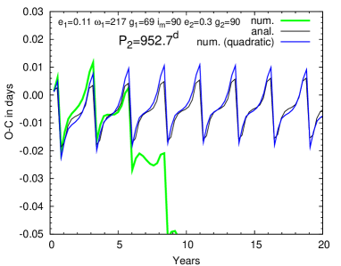
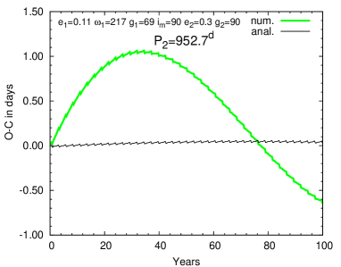
In the sample runs above a moderately hierarchic scenario $a_{2}\approx 22a_{1}$ was studied. In order to get some picture about the lower limit of the validity of our low-order, hierarchical approximation, we carried out further integrations for less hierarchic configurations. In Fig. 7 we show the results of some of these runs, which were carried out with the same initial conditions what were used in the middle panel of the first and last rows (coplanar and perpendicular cases, respectively) of Fig. 5, but for $P_{2}=1000$ days (i.e. $a_{2}\approx 4.8a_{1}$), $P_{2}=2000$ days ($a_{2}\approx 7.6a_{1}$), and $P_{2}\approx 952.7$ days ($a_{2}\approx 4.6a_{1}$), in which latter case the two planets orbit in $1:10$ mean motion resonance. In the left panels of Fig. 7 we plot 20-year-long intervals, while in the right ones century-long time-scales are shown. As one can see, on this latter time-scale, apse-node effects already reach or exceed the magnitude of the long period ones. This naturally arises from the fact that the typical time-scales of these latter high-amplitude perturbations are proportional to $P_{2}^{2}/P_{1}$, i.e. in the present cases these are $\sim 100\times$ faster than in the previously investigated case. Note, that for the sake of a better comparison, the analytical curves in the right panels were calculated with the inclusion of these apse-node terms, although the latter will be presented only in a forthcoming paper. Turning back to the 20-year-long integrations, one can see that the limit of the validity of the present approximation does strongly depend on the mutual inclination. While for the $i_{\mathrm{m}}=90\degr$ configurations the long period analytical results are in remarkably good agreement with the numerical curves even for $a_{2}<5a_{1}$ (left panels of third and forth rows), for the coplanar ($i_{\mathrm{m}}=0\degr$) case our approximation is clearly insufficient for such small $a_{2}/a_{1}$ ratios, and even for the doubled outer period case (i.e. $a_{2}\approx 8a_{1}$) the amplitude of the analytical curve is highly underestimated.

We also investigated the case of the $1:10$ mean-motion resonance. Our results for the perpendicular case are plotted in the last row. In this case the numerical integration shows very high amplitude apse-node scale variations that does not occur in the analytical curve. In order to get a better comparison between the analytical and numerical long-term variations in this case, we removed the apse-node effect from the numerical curve, by the use of a quadratic term, i.e. the (blue) $O-C$ curve was calculated in the form of

$$O-C=c_{0}+c_{1}E+c_{2}E^{2},$$ (59)

where $E$ is the cycle number. As one can see, this quadratic (blue) curve shows similar agreement with the analytical curve, which was found in the similar $a_{2}/a_{1}$ ratio non-resonant case. Consequently, we can state that our long term formulae are capable to produce the same accuracy even around mean-motion resonances.

Nevertheless, from these few arbitrary trial runs we cannot give general statements about the limits of our approximations. A detailed discussionof this point is postponed to a forthcoming paper, when we include the apse-node time scale terms.

While CoRoT-9b served as an illustration for the Transit Timing Variations in the low inner eccentricity case, our next sample exoplanet HD 80606b represents the extremely eccentric case.

Table 1: The initial parameters of the transiting planetary subsytems. (The masses are given in solar mass, periods in days, and angular elements in degrees.) The parameters are taken from Deeg et al. (2010) for CoRoT-9b, and from Pont et al. (2009) for HD~80606b. (Note that the argument of periastron ($\omega_{1}$) for the relative orbit of the planet around its host star differ by 180°from the value deduced from radial velocity data.)

$$\begin{array}[]{lllllll}\hline\cr\hline\cr\vskip 3.0pt plus 1.0pt minus 1.0pt\cr\mathrm{System}&m_{1}&m_{2}&P_{1}&e_{1}&\omega_{1}&i_{1}\\ \hline\cr\vskip 3.0pt plus 1.0pt minus 1.0pt\cr\mathrm{\object{CoRoT-9b}}&0.99&0.0008&95.2738&0.11&217&89.99\\ \mathrm{\object{HD~80606b}}&0.97&0.0038&111.4357&0.93&121&89.32\\ \hline\cr\vskip 3.0pt plus 1.0pt minus 1.0pt\cr\end{array}$$

4.2 HD 80606b

The high-mass gas giant exoplanet HD 80606b features an almost 4-month long period and an extremely eccentric orbit around its solar-type host-star. It was discovered spectroscopically by Naef et al. (2001). Recently both secondary occultation (with the Spitzer space telescope, Laughlin et al. 2009), and primary transit (Moutou et al. 2009; Fossey et al. 2009) have been detected. A thorough analysis of the collected data around the February 2009 primary transit led to the conclusion that there is a significant spin-orbit misalignment in the system, i.e. the orbital plane of HD 80606b fails to coincide with the equatorial plane of its host star (Pont et al. 2009). These facts suggest that this planet might be seen at an instant close to the maximum eccentricity phase of a Kozai cycle induced by a distant, inclined third companion (cf. Wu & Murray 2003; Fabrycky & Tremaine 2007). Note that although HD 80606 itself forms a binary with HD 80607, due to the large separation, one may expect a further, not so distant companion for an effective Kozai mechanism. Such a very distant companion may nevertheless play an indirect role in the initial triggering of the Kozai mechanism, by the effect described in Takeda et al. (2009). The most important parameters of the system are summarized in Table 1.

Due to its very high eccentricity, the periastron distance of this planet is $q_{1}=a_{1}(1-e_{1})\approx 0.03\mathrm{AU}$ at which distance the tidal forces and especially tidal dissipation should be effective. (As a comparison we note, that this separation corresponds to the semi-major axis of an approx. 2 day period orbit.) Furthermore, we can expect also a significant relativistic contribution to the apsidal motion. Although such circumstances do not invalidate the following conclusions (as the time-scale of these effects are significantly longer than the ones investigated) we nevertheless provide a quantitive estimation of their effects. Furthermore, the effect of dissipation will also be considered numerically, at the end of this section.

As is well known, the apsidal advance speed, averaged for one orbital revolution, can be written in the following form:

$$\dot{g}_{1}=A+B\cos 2g_{1},$$ (60)

where the non-zero contributions of the third-body, tidal and relativistic terms are as follows:

$$A_{3^{\mathrm{rd}}} = A_{\mathrm{L}}\frac{P_{1}}{P_{2}}\left(1-e_{1}^{2}\right)^{-1/2}\left[I^{2}-\frac{1}{5}\left(1-e_{1}^{2}\right)+\frac{2}{5}\left(1+\frac{3}{2}e_{1}^{2}\right)\frac{C_{1}}{C_{2}}I\right],$$

$$B_{3^{\mathrm{rd}}} = A_{\mathrm{L}}\frac{P_{1}}{P_{2}}\left(1-e_{1}^{2}\right)^{-1/2}\left[\left(1-e_{1}^{2}\right)-I^{2}-e_{1}^{2}\frac{C_{1}}{C_{2}}I\right],$$ (62)

$$A_{\mathrm{tidal}} = \frac{5{\cal{T}}}{2a_{1}^{5}}\frac{1+\frac{3}{2}e_{1}^{2}+\frac{1}{8}e_{1}^{4}}{\left(1-e_{1}^{2}\right)^{5}}+\frac{\cal{R}}{a_{1}^{2}\left(1-e_{1}^{2}\right)^{2}},$$ (63)

$$A_{\mathrm{rel}} = 6\pi\frac{Gm_{1}}{c^{2}a_{1}(1-e_{1}^{2})},$$ (64)

where

$$C_{1} = \frac{m_{1}m_{2}}{m_{12}}\sqrt{Gm_{12}a_{1}\left(1-e_{1}^{2}\right)},$$ (65)

$$= L_{1}\sqrt{1-e_{1}^{2}},$$

$$C_{2} = \frac{m_{12}m_{3}}{m_{123}}\sqrt{Gm_{123}a_{2}\left(1-e_{2}^{2}\right)},$$ (66)

$$= L_{2}\sqrt{1-e_{2}^{2}},$$

moreover,

$${\cal{T}} = 6\left(\frac{m_{2}}{m_{1}}k_{2}^{(1)}R_{1}^{5}+\frac{m_{1}}{m_{2}}k_{2}^{(2)}R_{2}^{5}\right),$$ (67)

$$= 6\frac{m_{2}}{m_{1}}R_{1}^{5}\left[k_{2}^{(1)}+k_{2}^{(2)}\left(\frac{\overline{\rho}_{1}}{\overline{\rho}_{2}}\right)^{2}\frac{R_{1}}{R_{2}}\right],$$

$${\cal{R}} = \frac{k_{2}^{(1)}R_{1}^{5}\omega^{2}_{z^{\prime}_{1}}}{Gm_{1}}+\frac{k_{2}^{(2)}R_{2}^{5}\omega^{2}_{z^{\prime}_{2}}}{Gm_{2}}$$ (68)

$$= \frac{3k_{2}^{(1)}}{4\pi G\overline{\rho}_{1}}v^{2}_{\mathrm{e}_{1}}+\frac{3k_{2}^{(2)}}{4\pi G\overline{\rho}_{2}}v^{2}_{\mathrm{e}_{2}}.$$

In these equations $m_{1}$, $R_{1}$, $\overline{\rho}_{1}$, $k_{2}^{(1)}$, $\omega_{z^{\prime}_{1}}$, $v_{\mathrm{e}_{1}}$ refer to the mass, radius, average density, first apsidal motion constant, uni-axial rotational angular velocity, and equatorial rotational velocity of the host star respectively, while subscript ₂ denotes the same quantities for the inner planet. Note also that the rotational term is valid only for non-aligned rotation, and consequently, it provides only a crude estimation for HD 80606b. Nevertheless, for the present purpose it seems satisfactory. First consider the third-body term. Substituting $\cos 2g=-1$, $I^{2}=3/5$,

$$\dot{g}_{3^{\mathrm{rd}}} = \frac{3\pi}{2}\frac{m_{3}}{m_{123}}\left(\frac{P_{1}}{P_{2}}\right)^{2}\left(1-e_{2}^{2}\right)^{-3/2}\left(1-e_{1}^{2}\right)^{-1/2}$$ (69)

$$\times\left[3e_{1}^{2}\pm\sqrt{\frac{3}{5}}\left(1+4e_{1}^{2}\right)\frac{L_{1}}{L_{2}}\sqrt{\frac{1-e_{1}^{2}}{1-e_{2}^{2}}}\right],$$

from which the last term usually omittable in hierarchical systems, since $C_{1}<<C_{2}$, which is more expressively true for high $e_{1}$. For example, in the present situation

$$\frac{C_{1}}{C_{2}}\approx 0.06\left(1-e_{2}^{2}\right)^{-1/2}.$$ (70)

So, for HD 80606b we obtain that:

$$\Delta g_{3^{\mathrm{rd}}}\approx 0\aas@@fstack{\circ}43\times\left(1-e_{2}^{2}\right)^{-3/2}\mathrm{century}^{-1}.$$ (71)

(This result is in excellent correspondance with Fig. 11.)

There are several uncertainties in the calculation of the tidal contribution. While the $k_{2}$ constant is relatively well-known for ordinary stars, it has a great ambiguity for exoplanets. Furthermore, we do know nothing about the rotational velocity of HD 80606b. So, according to the tables of Claret & Gimènez (1992) we set $k_{2}^{(1)}=0.02$ for the host star, and assumed $k_{2}^{(2)}=0.2$ for its planet, which is the same order of magnitude as for Jupiter and of WASP-12b (Campo et al. 2010). The stellar rotation was set to $V_{\mathrm{rot}}=1.8\mathrm{\leavevmode\nobreak\ km}\,\mathrm{s}^{-1}$ (i.e. $P_{\mathrm{rot}}=27\aas@@fstack{d}5$; $\omega_{z^{\prime}_{1}}=0.228\mathrm{\leavevmode\nobreak\ day}^{-1}$) (Fischer & Valenti 2005), while for the planet we supposed (arbitrarily) a one-day rotation period, i.e. $\omega_{z^{\prime}_{1}}=6.283\mathrm{\leavevmode\nobreak\ day}^{-1}$. By the use of these values, the classical tidal contribution to the apsidal motion becomes

$$\Delta g_{\mathrm{tidal}}\approx 0\aas@@fstack{\circ}007\mathrm{\leavevmode\nobreak\ century}^{-1},$$ (72)

which can be neglected.

Finally, the relativistic contribution is estimated to be:

$$\Delta g_{\mathrm{rel}}\approx 0\aas@@fstack{\circ}06\mathrm{\leavevmode\nobreak\ century}^{-1},$$ (73)

i.e. it is smaller by one magnitude than the third-body term, and consequently, does also not play any important role.

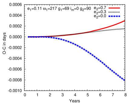
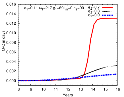
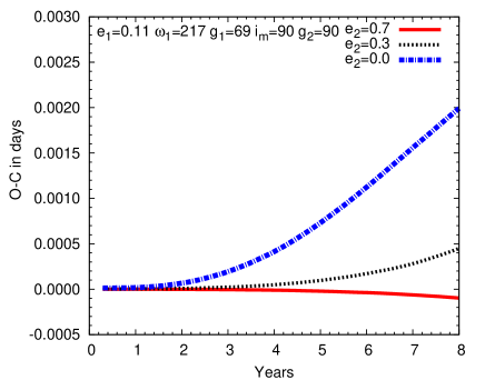
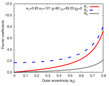
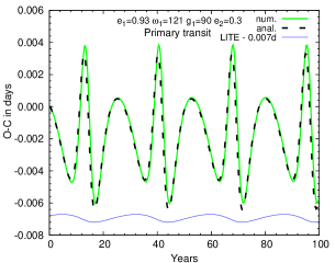
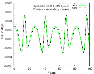
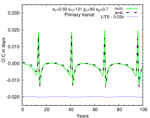
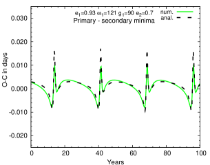
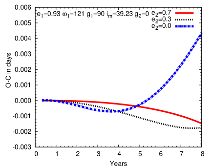
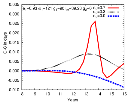
Returning to the $P_{2}$ time-scale variations of the TTV-s, we carried out our calculations and integration runs with the supposition that a second, similar mass giant planet is the source of this comet-like orbit, which is seen in the instant of the maximum eccentricity phase of the Kozai-cycle. Consequently, we set $g_{1}=90$°, and $i_{\mathrm{m}}=39\aas@@fstack{\circ}23$. With these values from the sixth order formula we get $A_{\cal{M}}=-0.38$, $A_{\cal{S}}=1.69$ for primary transits, and $A_{\cal{M}}=-1.06$, $A_{\cal{S}}=1.72$ for secondary occultations. Consequently, for primary transits the $O-C$ is evidently dominated by the ${\cal{S}}$-term. (The negative $A_{\cal{M}}$ indicates a simple 180°phase-shift.) In Fig. 8 the $A_{1,2,3}$ amplitudes are plotted as a function of the outer eccentricity ($e_{2}$). Due to the more than four and a half-times larger primary transit ${\cal{S}}$ amplitude, the $g_{2}$ dependence of the amplitudes here are weak, and therefore we show only $A_{1,2,3}$-s for $g_{2}=0$°.

Figure 8: The $A_{1,2,3}$ amplitudes for HD 80606b for primary transits (left), and secondary occultations (right), supposing that the planet is seen at the instant of the maximum phase of a Kozai-cycle.

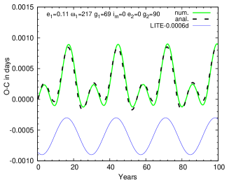
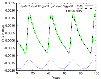
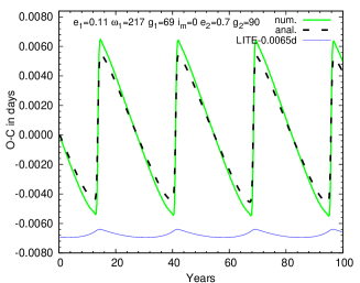
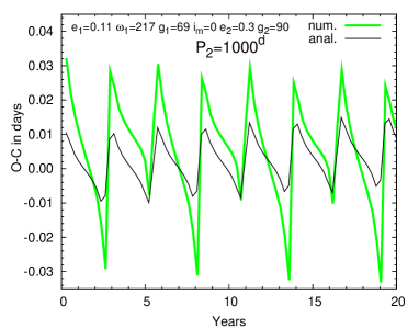
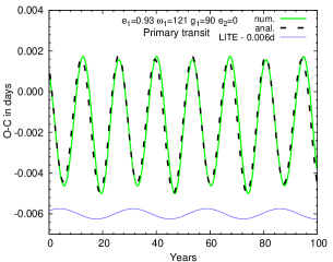
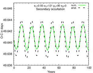
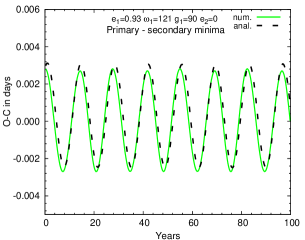
In Fig. 9 we present both the numerically generated short-term $O-C$ curves, as well as the analytically calculated cases up to the sixth order in eccentricity (see Appendix) for three different eccentricities ($e_{2}=0$, 0.3, 0.7) of the outer perturber’s orbit. We plotted the $O-C$-s for both primary transits and secondary occultations. Also shown are the corresponding primary minus secondary curves.

As one can see, the sixth order formulae gave satisfactory results even for such high eccentricities, although the analytical amplitudes are somewhat overestimated. Nevertheless, a more detailed analysis shows that the accuracy of our formulae for such high inner eccentricities strongly depends on the other orbital parameters. This is illustrated even in the present situation, where, for the secondary-occultation curves, (which correspond to $\omega_{1}=301$°), the discrepancies are clearly larger. From this point of view, the $e_{2}=0$ case (first row) is the more interesting, as in this situation, due to the non-zero, very similar $A_{\mathrm{\cal{S}}}=A_{2}$ amplitudes, we would expect almost identical $O-C$ curves (since the dashed analytical ones are very similar), but this, in fact, is not the case.

Figure 9: Transit timing variatons caused by a hypothetical $P_{2}=10\,000$ day-period $m_{3}=0.005M_{\mathrm{\sun}}(\approx 5M_{\mathrm{J}})$ mass third companion for HD 80606b at the maximum eccentricity phase of the induced Kozai-cycles. Top: $e_{2}=0$; middle: $e_{2}=0.3$; bottom: $e_{2}=0.7$ ($g_{2}=0\degr$ in all cases); left panels: primary transits; middle panels: secondary occultations; right panels: primary minus secondary difference. See text for further details. (For better comparison the curves are corrected for the different average transit periods, and zero point shifts.)

Considering the case of fastest possible detection of the amplitudes, in Fig. 10 we plotted also the first and second 8 years of the three primary transit $O-C$ curves, shown in Fig. 9. The transiting periods for each curves were calculated on the usual, observational manner, i.e. the time interval between the first (some) transits were used. According to Fig. 10, in the first 8 year, i.e. after the apastron of the outer body, the fastest detection would be possible in the smallest (total) amplitude circular third body-case, while the curvature of the highly eccentric curve is so small, that it needs almost 7 years to exceed the $0\aas@@fstack{d}001$ difference which could promise certain detection. (Of course, this is a non-realistic ideal case, when all the transits are measured, without any observational error.) Around periastron (right panel), the situation is completely different, similarly to the case of CoRoT-9b.

Figure 10: The first and second 8 years of the left panels of Fig. 9. The periods of the individual curves was set equal to the each initial transiting periods.

Figure 11: Dynamical evolution of the orbital elements of HD 80606b in the presence of a hypothetical $P_{2}=10\,000$ day-period $m_{3}=0.005M_{\mathrm{\sun}}(\approx 5M_{\mathrm{J}})$ mass third companion. The initial orbital elements correspond to the last row of Fig. 9. Red curves: tidal effects and dissipation are considered; blue curves: three point-mass model. (Relativistic contributions are omitted.) Note, the semi-major axis ($a_{1}$) is given in R_☉.

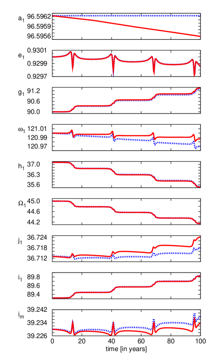
We also carried out numerical integrations to investigate the possible orbital evolution of HD 80606b in the presence of such a perturber. We have shown that both relativistic and tidal effects are omittable in the present configuration of the system. However, this assumption is only correct in those cases where tidally forced dissipation is not considered. Consequently, we integrated the dynamical evolution of the system including both tidal effects (both dissipative and conservative tidal terms), and without them (i.e. in the frame of pure three, point-mass gravitational interactions). The equations of the motion (including tidal and dissipative terms, and stellar rotation) are given in Borkovits et al. (2004), where the description of our integrator can also be found. In the dissipative case our dissipation constant was selected in such a way that it produced $\Delta t_{1}\approx 2\aas@@fstack{d}16\times 10^{-7}$ tidal lag-time for the host-star, and $\Delta t_{1}\approx 5\aas@@fstack{d}21\times 10^{-4}$ for the planet, which are equivalent to $Q_{1}\approx 4.1\times 10^{7}$, $Q_{2}\approx 1.7\times 10^{4}$ dissipation parameters, respectively. Fig. 11 shows the variation of most of the orbital elements (both dynamical and observational) for 100 and 1 million years in the dynamically most-excited $e_{2}=0.7$ case. Thick lines represent the dissipative case, while thin curves show the point-mass result. The century-long left panel demonstrates, that apart from the shrinking semi-major axis, there is no detectable variation in the orbital elements during such a short time-interval. And, of course, if this is true for the extremum of the Kozai cycle, it is more expressly valid for other situations, as this phase produces the fastest orbital element variations. Furthermore, on such a short time-scale the orbital variations in a point-mass or non-Keplerian, tidal framework are indistinguishable. (Again, we do not take into account the semi-major axis.) This provides further verification of the effects previously-discussed, namely that we neglected the tidal and relativistic effects completely, and considered all the orbital elements as constant.

Now, we consider orbital shrinking due to dissipation. As one can see, in the present situation the decrease in $a_{1}$ during the first 100 years is $\Delta a_{1}\approx 6\times 10^{-4}\mathrm{\leavevmode\nobreak\ R}_{\mathrm{\sun}}$. Converting this into a period variation suggests $\Delta P_{1}\approx 10^{-3}\mathrm{\leavevmode\nobreak\ d}$. This gives for one transiting period a $\dot{P}_{1}\approx 3\times 10^{-6}\mathrm{\leavevmode\nobreak\ day\,cycle}^{-1}$ rate. From the point of view of an eclipsing binary observer, this is an incredibly large value. For comparison, a typical secular period variation rate measured for many of the eclipsing binaries is about $10^{-9}-10^{-11}\mathrm{\leavevmode\nobreak\ day\,cycle}^{-1}$. Such a high rate would produce $0\aas@@fstack{d}001$ departure in transit time during $\sim 26$ cycles, i.e. during approximately 8 years. Note, this period variation ratio is close to that ratio produced by typical long-term perturbations within a few years. This illustrates that if the data-length is significantly shorter than the period of the long-term periodic perturbations, then the effect arose from such perturbations, and other effects, coming from i.e. orbital shrinking can overlap each-other, and as a result they can be misinterpreted easily. (The question of such kinds of misinterpretations or false identifications were considered in general in Sect. 2 of Borkovits et al. 2005).

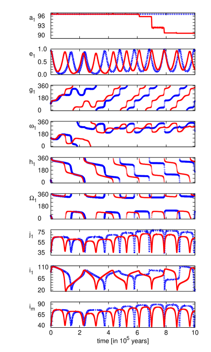
Finally, we consider the right panel of Fig. 11, which illustrates the frequently mentioned Kozai-mechanism (with and without tidal friction) in operation. Note, that in the present situation due to the high outer eccentricity, and as well as the relatively weak hierarchicity of the system (i.e. $a_{1}/a_{2}\approx 0.05$) the higher order terms of the perturbation function are also significant, which results in very different consecutive cycles even in the point-mass case, too. This manifests not only as different periods and maximum eccentricities, but e.g. in the fact that the argument of (dynamical) periastron ($g_{1}$) shows both circulation, and libration, alternately (cf. Ford et al. 2000). Nevertheless, the detailed investigation of the apse-node timescale behaviour of the TTV, as well as other orbital elements and observables will be the subject of a succeeding paper.

5 Conclusions

We have studied the long-term $P_{2}$ time-scale transit timing variations in transiting exoplanetary systems which feature a further, more distant ($a_{2}>>a_{1}$) either planetary, or stellar companion. We gave the analytical form of the $O-C$ diagram which describes such TTV-s. Our result is an extention of our previous work, namely Borkovits et al. (2003) for arbitrary orbital elements of both the inner transiting planet and the outer companion. We showed that the dependence of the $O-C$ on the orbital and physical parameters can be separated into three parts. Two of these are independent of the real physical parameters (i.e. masses, separations, periods) of a concrete system, and depend only on dimensionless orbital elements, and so, can be analysed in general. For the two other kinds of parameters, which are amplitudes and phases of trigonometric functions, we separated the orbital elements of the inner from the outer planet. The practical importance of such a separation is that in the case of any actual transiting exoplanets, if eccentricity ($e_{1}$) and the observable argument of periastron ($\omega_{1}$) are known e.g. from spectroscopy, then the main characteristics of any, caused by a possible third-body, transit timing variations can be mapped simply by the variation of two free parameters (dynamical, relative argument of periastron, $g_{1}$, and mutual inclination, $i_{\mathrm{m}}$), which then can be refined by the use of the other, derived parameters, including two additional parameters fot the possible third body (eccentricity, $e_{2}$, and dynamical, relative argument of periastron, $g_{2}$). Moreover, as the physical attributes of a given system occur only as scaling parameters, the real amplitude of the $O-C$ can also be estimated for a given system, simply as a function of the $m_{3}/P_{2}$ ratio.

At this point it would be no without benefit to compare our results with the conclusions of Nesvorný & Morbidelli (2008) and Nesvorný (2009). These authors investigated the same problem, i.e. the fast detectability of outer perturbing planets, and determination of their orbital and physical parameters from their perturbations on the transit timing of the inner planet, by the help of the analytical description of the perturbed transiting $O-C$ curve. For the mathematical description they used the explicite perturbation theory of Hori (1966) and Deprit (1969) based on canonical transformations and on the use of Lie-series. This theory does not require the hierarchical assumption, i.e. the $\alpha=a_{1}/a_{2}$ parameter, although less than unity, is not required to be small. This suggests a somewhat greater generality of the results, i.e. it is well applicable systems similar to our solar system. Nevertheless, perhaps a small disadvantage of this method with respect to the hierarchical approximation is, that for large mutual inclinations the number of terms in the perturbation function needed for a given accuracy grows very fast, while our formulae have the same accuracy even for the largest mutual inclinations. There is also a similar discomfort in the case of high eccentricities, in which case the general formulae of Nesvorný (2009) are more sensitive for these parameters than in the hierarchical case. For example, we could reproduce satisfactory accuracy even for $e_{1}=0.9$, in which case the classical formulae are divergent. (Note, that although in this paper we concentrate only on the long period perturbations, the same is valid for the apse-node time-scale variations, as will be illustrated in the next paper.) As a conclusion, the greater generality of the method used by Nesvorný & Morbidelli (2008) and Nesvorný (2009) beyond the evident non-hierarchical configurations is well (or even better) applicable also in the nearly coplanar case, especially when the inner orbit is nearly circular (in which strict case the first order hierarchical approximation becomes insufficient, Ford et al. 2000, see e.g), but in other cases, as far as the hierarchical assumption is satisfied, this latter could give a faster and simpler method. Furthermore, since in the hierarchical approximation, the principal small parameter in the perturbation equations is the ratio of the separations instead of the mass-ratio, these formulae are valid for stellar mass objects as well, and can also be applicable for planets orbiting an S-type orbit in binary stars, or even for hierarchical triple stellar systems.

We analysed the above-mentioned dimensionless amplitudes for different arbitrary initial parameters, as well as for two concrete systems CoRoT-9b and HD 80606b. We found in general, that while the shape of the $O-C$ strongly varies with the angular orbital elements, the net amplitude (departing from some specific configurations) depends only weakly on these elements, but strongly on the eccentricities. Nevertheless, we found some situations around $i_{\mathrm{m}}=45$°for the specific case of CoRoT-9b, where the $O-C$ almost disappeared.

We used CoRoT-9b and HD 80606b for case studies. Both giant planets revolve on several month-period orbits. The former has an almost circular orbit, while the latter has a comet-like, extremely eccentric orbit. These large period systems are ideal for searching for further perturbing components, as the amplitude of the $O-C$ is multiplied by $P_{1}^{2}/P_{2}$ and consequently, as the magnitude of the perturbations determined by $P_{1}/P_{2}$, the same amplitude perturbations cause a better detectable effect, if the characteristic size of the system (i.e. $P_{1}$) is larger.

We considered also the question of detection, as well as the correct identification of such perturbations. We emphasize again, that the $O-C$ curve is a very effective tool for detection of any period variations, due to its cumulative nature. Nevertheless, some care is necessary. First, it has to be kept in mind, that the detectability of a period variation depends on the curvature of the $O-C$ curve. (If the plotted $O-C$ is simply a straight line, with any slope, it means that the period is constant, which is known with an error equal to that slope.) This implies that the interval which is necessary to detect the period variation coming from a periodic phenomenon depends more strong on which phase is observed than on the amplitude of the total variation. (We illustrated this possibility for both system sampled.) We illustrated also, that in the case of a very eccentric third companion the fastest rate period variation lasts a very short interval, which consists of only a few transit events. This emphasizes the importance of observing all possible transits (and, of course occultation) events, with great accuracy. A further question is the possible misinterpretation of the $O-C$ diagram. For example, as was shown, in the HD 80606b system we can expect a secular period change due to tidal dissipation, which has the same order of magnitude than might have been measured due to the periodic perturbations of some hypothetical third body as our sample. These two types of perturbations could be separated in two different ways. One way is simply a question of time. In the case of a sufficiently long observing window, a periodic pertubation would separate from a secular one, which would produce a parabola-like $O-C$ continuously. But, there is also a faster possibility. In the case that not only primary transits, but also secondary occultations are observed with similar frequency and accuracy, then, on subtracting the two (primary and secondary) $O-C$ curves from each-other, the secular change, i.e. the effect of dissipation would disappear, since it is similar for primary transits and secondary occultations. This fact also makes desirable the collection of as many as possible occultation observations too.

Appendix A Relation between the observable, and the dynamical orbital elements.

The start of the paper remarked that some of the relations between the elements given in this section are valid strictly in the presented form only for the situation shown in Fig. 1. According to the actual orientations of the orbital planes, the spherical triangle (with sides $u_{\mathrm{m1}}$, $u_{\mathrm{m2}}$, $\Omega_{1}-\Omega_{2}$) could be oriented in different ways, and so, some precise discussion are necessary, which is omitted in the present appendix.

The relation between the pericentrum arguments are as follows:

$$\omega_{1} = g_{1}+u_{\mathrm{m1}},$$ (74)

$$\omega_{2} = g_{2}+u_{\mathrm{m2}}+180\degr.$$ (75)

Consequently, the true longitudes measured from the sky ($u$) and from the intersection of the two orbital planes ($w$) are:

$$u_{1} = v_{1}+\omega_{1},$$ (76)

$$u_{2} = v_{2}+\omega_{2},$$ (77)

$$w_{1} = v_{1}+g_{1},$$ (78)

$$= u_{1}-u_{\mathrm{m1}},$$ (79)

$$w_{2} = v_{2}+g_{2}+180\degr,$$ (80)

$$= u_{2}-u_{\mathrm{m2}}.$$ (81)

There are two relations between the mutual inclination ($i_{\mathrm{m}}$) and the two dynamical inclinations ($j_{1,2}$). One of these is trivial, while the second comes from the relation of the inclinations to the orbital angular momenta. The trivial case is

$$i_{\mathrm{m}}=j_{1}+j_{2},$$ (82)

while the non-trivial case comes from the fact, that

$$\cos j_{1} = \frac{\@vec{C}\@vec{C}_{1}}{CC_{1}},$$ (83)

$$\sin j_{1} = \frac{|\@vec{C}\times\@vec{C}_{1}|}{CC_{1}},$$ (84)

i.e.

$$\cos j_{1} = \frac{C_{1}}{C}+\frac{C_{2}}{C}I,$$ (85)

$$\sin j_{1} = \frac{C_{2}}{C}\sin i_{\mathrm{m}},$$ (86)

where $\@vec{C}_{1,2}$ represents the orbital angular momentum vector of the two orbits, $\@vec{C}$ the net orbital angular momentum vector, and

$$C_{1} = \frac{m_{1}m_{2}}{m_{12}}\sqrt{Gm_{12}a_{1}\left(1-e_{1}^{2}\right)},$$ (87)

$$C_{2} = \frac{m_{12}m_{3}}{m_{123}}\sqrt{Gm_{123}a_{2}\left(1-e_{2}^{2}\right)},$$ (88)

$$C = C_{1}\cos j_{1}+C_{2}\cos j_{2}.$$ (89)

(The rotational angular momenta were neglected.) At this point we remark that for hierarchical systems it is a very reasonable to assume

$$C_{1}\cos j_{1}=\mathrm{constant},$$ (90)

(since the first order, doubly averaged Hamiltonian of such systems does not contain its conjugated variable, $h_{1}$), which property, together with the constancy of the semi-major axis connects the eccentricity ($e_{1}$) with the dynamical inclination ($j_{1}$).

Further relations can be written by the use of the several identities of spherical triangles. For example:

$$\cos i_{\mathrm{m}} = \cos i_{1}\cos i_{2}+\sin i_{1}\sin i_{2}\cos(\Omega_{2}-\Omega_{1}),$$ (91)

$$\sin i_{\mathrm{m}}\sin u_{\mathrm{m2}} = \sin i_{1}\sin(\Omega_{2}-\Omega_{1}),$$ (92)

$$\sin i_{\mathrm{m}}\sin u_{\mathrm{m1}} = \sin i_{2}\sin(\Omega_{2}-\Omega_{1}),$$ (93)

$$\sin i_{\mathrm{m}}\cos u_{\mathrm{m2}} = -\cos i_{1}\sin i_{2}+\sin i_{1}\cos i_{2}\cos(\Omega_{2}-\Omega_{1}),$$ (94)

$$\sin i_{\mathrm{m}}\cos u_{\mathrm{m1}} = \cos i_{2}\sin i_{1}-\sin i_{2}\cos i_{1}\cos(\Omega_{2}-\Omega_{1}),$$ (95)

and similar ones can be written for the two smaller spherical triangles. Finally, in hierarchical systems usually $C_{2}>>C_{1}$, so we can take the following as a first approximation:

$$j_{1} = i_{\mathrm{m}},$$ (96)

$$j_{2} = 0,$$ (97)

$$i_{0} = i_{2},$$ (98)

$$h_{1} = u_{\mathrm{m2}}.$$ (99)

We note that in Fig. 1, for practical reasons, we chose the intersection of the invariable plane and the sky for the arbitrary starting point of the observable nodes ($\Omega_{1}$, $\Omega_{2}$). Traditionally, in astrometry, these quantities are measured from north to east on the sky, nevertheless such an approximation is valid since the $\Omega$-s only appear in the equations in the form of their differences, and derivatives. (Nodes cannot be determined from photometry and spectroscopy, as both the light curves and the radial velocity curves are invariant for any orientation of the orbital planes projected onto the sky.)

Appendix B The derivatives used for calculating the long-period dynamical $O-C$ up to sixth order in $e_{1}$

The derivatives of the indirect terms are as follows:

$$\frac{\mathrm{d}{e_{1}\cos\omega_{1}}}{\mathrm{d}{v_{2}}} = A_{\mathrm{L}}\left(1+e_{2}\cos v_{2}\right)\left\{(1-e_{1}^{2})^{1/2}\left\{-\frac{3}{5}e_{1}\sin\omega_{1}\left[\left(I^{2}-\frac{1}{3}\right)+\left(1-I^{2}\right)\cos(2v_{2}+2g_{2})\right]\right.\right.$$ (100)

$$-e_{1}\sin(\omega_{1}-2g_{1})\left[\left(1-I^{2}\right)+\left(1+I^{2}\right)\cos(2v_{2}+2g_{2})\right]$$

$$\left.-e_{1}\cos(\omega_{1}-2g_{1})2I\sin(2v_{2}+2g_{2})\right\}$$

$$+\frac{\sin i_{\mathrm{m}}\cot i_{1}}{\left(1-e_{1}^{2}\right)^{1/2}}\left\{\left[\frac{2}{5}\left(1+\frac{3}{2}e_{1}^{2}\right)\cos u_{\mathrm{m1}}-e_{1}^{2}\cos(2g_{1}+u_{\mathrm{m1}})\right]e_{1}\sin\omega_{1}I\left[1-\cos(2v_{2}+2g_{2})\right]\right.$$

$$\left.\left.+\left[\frac{2}{5}\left(1+\frac{3}{2}e_{1}^{2}\right)\sin u_{\mathrm{m1}}+e_{1}^{2}\sin(2g_{1}+u_{\mathrm{m1}})\right]e_{1}\sin\omega_{1}\sin(2v_{2}+2g_{2})\right\}\right\},$$

$$\frac{\mathrm{d}{e_{1}^{2}f_{3}(e_{1})\sin 2\omega_{1}}}{\mathrm{d}{v_{2}}} = A_{\mathrm{L}}\left(1+e_{2}\cos v_{2}\right)\left\{(1-e_{1}^{2})^{1/2}\left\{\frac{6}{5}e_{1}^{2}f_{3}\cos 2\omega_{1}\left[\left(I^{2}-\frac{1}{3}\right)+\left(1-I^{2}\right)\cos(2v_{2}+2g_{2})\right]\right.\right.$$ (101)

$$+\left[2e_{1}^{2}f_{4}\cos(2\omega_{1}-2g_{1})-\frac{1}{6}e_{1}^{4}f_{5}\cos(2\omega_{1}+2g_{1})\right]\left[\left(1-I^{2}\right)+\left(1+I^{2}\right)\cos(2v_{2}+2g_{2})\right]$$

$$\left.-\left[2e_{1}^{2}f_{4}\sin(2\omega_{1}-2g_{1})+\frac{1}{6}e_{1}^{4}f_{5}\sin(2\omega_{1}+2g_{1})\right]2I\sin(2v_{2}+2g_{2})\right\}$$

$$+\frac{\sin i_{\mathrm{m}}\cot i_{1}}{\left(1-e_{1}^{2}\right)^{1/2}}f_{3}\left\{\left[-\frac{4}{5}\left(1+\frac{3}{2}e_{1}^{2}\right)\cos u_{\mathrm{m1}}+2e_{1}^{2}\cos(2g_{1}+u_{\mathrm{m1}})\right]e_{1}^{2}\cos 2\omega_{1}I\left[1-\cos(2v_{2}+2g_{2})\right]\right.$$

$$\left.\left.-\left[\frac{4}{5}\left(1+\frac{3}{2}e_{1}^{2}\right)\sin u_{\mathrm{m1}}+2e_{1}^{2}\sin(2g_{1}+u_{\mathrm{m1}})\right]e_{1}^{2}\cos 2\omega_{1}\sin(2v_{2}+2g_{2})\right\}\right\},$$

$$\frac{\mathrm{d}{e_{1}^{3}f_{6}(e_{1})\cos 3\omega_{1}}}{\mathrm{d}{v_{2}}} = A_{\mathrm{L}}\left(1+e_{2}\cos v_{2}\right)\left\{(1-e_{1}^{2})^{1/2}\left\{-\frac{9}{5}e_{1}^{3}f_{6}\sin 3\omega_{1}\left[\left(I^{2}-\frac{1}{3}\right)+\left(1-I^{2}\right)\cos(2v_{2}+2g_{2})\right]\right.\right.$$ (102)

$$-\left[3e_{1}^{3}f_{7}\sin(3\omega_{1}-2g_{1})-\frac{3}{8}e_{1}^{5}\sin(3\omega_{1}+2g_{1})\right]\left[\left(1-I^{2}\right)+\left(1+I^{2}\right)\cos(2v_{2}+2g_{2})\right]$$

$$-\left.\left[3e_{1}^{3}f_{7}\cos(3\omega_{1}-2g_{1})+\frac{3}{8}e_{1}^{5}\cos(3\omega_{1}+2g_{1})\right]2I\sin(2v_{2}+2g_{2})\right\}$$

$$+\frac{\sin i_{\mathrm{m}}\cot i_{1}}{\left(1-e_{1}^{2}\right)^{1/2}}f_{6}\left\{\left[\frac{6}{5}\left(1+\frac{3}{2}e_{1}^{2}\right)\cos u_{\mathrm{m1}}-3e_{1}^{2}\cos(2g_{1}+u_{\mathrm{m1}})\right]e_{1}^{3}\sin 3\omega_{1}I\left[1-\cos(2v_{2}+2g_{2})\right]\right.$$

$$\left.\left.+\left[\frac{6}{5}\left(1+\frac{3}{2}e_{1}^{2}\right)\sin u_{\mathrm{m1}}+3e_{1}^{2}\sin(2g_{1}+u_{\mathrm{m1}})\right]e_{1}^{3}\sin 3\omega_{1}\sin(2v_{2}+2g_{2})\right\}\right\},$$

$$\frac{\mathrm{d}{e_{1}^{4}f_{8}(e_{1})\sin 4\omega_{1}}}{\mathrm{d}{v_{2}}} = A_{\mathrm{L}}\left(1+e_{2}\cos v_{2}\right)\left\{(1-e_{1}^{2})^{1/2}\left\{\frac{12}{5}e_{1}^{4}f_{8}\cos 4\omega_{1}\left[\left(I^{2}-\frac{1}{3}\right)+\left(1-I^{2}\right)\cos(2v_{2}+2g_{2})\right]\right.\right.$$ (103)

$$+\left[4e_{1}^{4}f_{5}\cos(4\omega_{1}-2g_{1})-\frac{3}{5}e_{1}^{6}\cos(4\omega_{1}+2g_{1})\right]\left[\left(1-I^{2}\right)+\left(1+I^{2}\right)\cos(2v_{2}+2g_{2})\right]$$

$$\left.-\left[4e_{1}^{4}f_{5}\sin(4\omega_{1}-2g_{1})+\frac{3}{5}e_{1}^{6}\sin(4\omega_{1}+2g_{1})\right]2I\sin(2v_{2}+2g_{2})\right\}$$

$$+\frac{\sin i_{\mathrm{m}}\cot i_{1}}{\left(1-e_{1}^{2}\right)^{1/2}}f_{8}\left\{\left[-\frac{8}{5}\left(1+\frac{3}{2}e_{1}^{2}\right)\cos u_{\mathrm{m1}}+4e_{1}^{2}\cos(2g_{1}+u_{\mathrm{m1}})\right]e_{1}^{4}\cos 4\omega_{1}I\left[1-\cos(2v_{2}+2g_{2})\right]\right.$$

$$\left.\left.-\left[\frac{8}{5}\left(1+\frac{3}{2}e_{1}^{2}\right)\sin u_{\mathrm{m1}}+4e_{1}^{2}\sin(2g_{1}+u_{\mathrm{m1}})\right]e_{1}^{4}\cos 4\omega_{1}\sin(2v_{2}+2g_{2})\right\}\right\},$$

$$\frac{\mathrm{d}{e_{1}^{5}\cos 5\omega_{1}}}{\mathrm{d}{v_{2}}} = A_{\mathrm{L}}\left(1+e_{2}\cos v_{2}\right)\left\{(1-e_{1}^{2})^{1/2}\left\{-3e_{1}^{5}\sin 5\omega_{1}\left[\left(I^{2}-\frac{1}{3}\right)+\left(1-I^{2}\right)\cos(2v_{2}+2g_{2})\right]\right.\right.$$ (104)

$$-5e_{1}^{5}\sin(5\omega_{1}-2g_{1})\left[\left(1-I^{2}\right)+\left(1+I^{2}\right)\cos(2v_{2}+2g_{2})\right]$$

$$\left.-5e_{1}^{5}\cos(5\omega_{1}-2g_{1})2I\sin(2v_{2}+2g_{2})\right\}$$

$$+\frac{\sin i_{\mathrm{m}}\cot i_{1}}{\left(1-e_{1}^{2}\right)^{1/2}}\left\{\left[2\left(1+\frac{3}{2}e_{1}^{2}\right)\cos u_{\mathrm{m1}}-5e_{1}^{2}\cos(2g_{1}+u_{\mathrm{m1}})\right]e_{1}^{5}\sin 5\omega_{1}I\left[1-\cos(2v_{2}+2g_{2})\right]\right.$$

$$\left.\left.+\left[2\left(1+\frac{3}{2}e_{1}^{2}\right)\sin u_{\mathrm{m1}}+5e_{1}^{2}\sin(2g_{1}+u_{\mathrm{m1}})\right]e_{1}^{5}\sin 5\omega_{1}\sin(2v_{2}+2g_{2})\right\}\right\},$$

$$\frac{\mathrm{d}{e_{1}^{6}\sin 6\omega_{1}}}{\mathrm{d}{v_{2}}} = A_{\mathrm{L}}\left(1+e_{2}\cos v_{2}\right)\left\{(1-e_{1}^{2})^{1/2}\left\{\frac{18}{5}e_{1}^{6}\cos 6\omega_{1}\left[\left(I^{2}-\frac{1}{3}\right)+\left(1-I^{2}\right)\cos(2v_{2}+2g_{2})\right]\right.\right.$$ (105)

$$+6e_{1}^{6}\cos(6\omega_{1}-2g_{1})\left[\left(1-I^{2}\right)+\left(1+I^{2}\right)\cos(2v_{2}+2g_{2})\right]$$

$$\left.-6e_{1}^{6}\sin(6\omega_{1}-2g_{1})2I\sin(2v_{2}+2g_{2})\right\}$$

$$+\frac{\sin i_{\mathrm{m}}\cot i_{1}}{\left(1-e_{1}^{2}\right)^{1/2}}f_{8}\left\{\left[-\frac{12}{5}\left(1+\frac{3}{2}e_{1}^{2}\right)\cos u_{\mathrm{m1}}+6e_{1}^{2}\cos(2g_{1}+u_{\mathrm{m1}})\right]e_{1}^{4}\cos 6\omega_{1}I\left[1-\cos(2v_{2}+2g_{2})\right]\right.$$

$$\left.\left.-\left[\frac{12}{5}\left(1+\frac{3}{2}e_{1}^{2}\right)\sin u_{\mathrm{m1}}+6e_{1}^{2}\sin(2g_{1}+u_{\mathrm{m1}})\right]e_{1}^{6}\cos 6\omega_{1}\sin(2v_{2}+2g_{2})\right\}\right\}.$$

The direct terms are coming from ($a^{3/2}e^{m}\cos(nv)$ and $\dot{\Omega}\cos i_{1}$) are as follows:

$$\left(\frac{\mathrm{d}e_{1}\cos v}{\mathrm{d}v_{2}}\right)_{\mathrm{dir}} = A_{\mathrm{L}}\left(1+e_{2}\cos v_{2}\right)(1-e_{1}^{2})^{1/2}\left\{-\frac{2}{5}\left(1+\frac{1}{2}e_{1}^{2}\right)\left[\left(I^{2}-\frac{1}{3}\right)+\left(1-I^{2}\right)\cos(2v_{2}+2g_{2})\right]\right.$$ (106)

$$-e_{1}^{2}\cos 2g_{1}\left[\left(1-I^{2}\right)+\left(1+I^{2}\right)\cos(2v_{2}+2g_{2})\right]$$

$$\left.-e_{1}^{2}\sin 2g_{1}2I\sin(2v_{2}+2g_{2})\right\}+...,$$

$$\left(\frac{\mathrm{d}e_{1}^{2}f_{3}(e_{1})\cos 2v}{\mathrm{d}v_{2}}\right)_{\mathrm{dir}} = A_{\mathrm{L}}\left(1+e_{2}\cos v_{2}\right)(1-e_{1}^{2})^{1/2}\left\{\frac{3}{5}e_{1}^{2}\left(1+\frac{1}{4}e_{1}^{2}+\frac{1}{18}e_{1}^{4}\right)\left[\left(I^{2}-\frac{1}{3}\right)+\left(1-I^{2}\right)\cos(2v_{2}+2g_{2})\right]\right.$$ (107)

$$-\frac{1}{5}e_{1}^{2}\left(1-\frac{53}{12}e_{1}^{2}-\frac{3}{2}e_{1}^{4}\right)\cos 2g_{1}\left[\left(1-I^{2}\right)+\left(1+I^{2}\right)\cos(2v_{2}+2g_{2})\right]$$

$$\left.-\frac{1}{5}e_{1}^{2}\left(1-\frac{53}{12}e_{1}^{2}-\frac{3}{2}e_{1}^{4}\right)\sin 2g_{1}2I\sin(2v_{2}+2g_{2})\right\}+...,$$

$$\left(\frac{\mathrm{d}e_{1}^{3}f_{6}(e_{1})\cos 3v}{\mathrm{d}v_{2}}\right)_{\mathrm{dir}} = A_{\mathrm{L}}\left(1+e_{2}\cos v_{2}\right)(1-e_{1}^{2})^{1/2}\left\{-\frac{3}{5}e_{1}^{4}\left(1+\frac{1}{2}e_{1}^{2}\right)\left[\left(I^{2}-\frac{1}{3}\right)+\left(1-I^{2}\right)\cos(2v_{2}+2g_{2})\right]\right.$$ (108)

$$+\frac{1}{5}e_{1}^{2}\left(1+e_{1}^{2}-\frac{49}{16}e_{1}^{4}\right)\cos 2g_{1}\left[\left(1-I^{2}\right)+\left(1+I^{2}\right)\cos(2v_{2}+2g_{2})\right]$$

$$\left.+\frac{1}{5}e_{1}^{2}\left(1+e_{1}^{2}-\frac{49}{16}e_{1}^{4}\right)\sin 2g_{1}2I\sin(2v_{2}+2g_{2})\right\}+...,$$

$$\left(\frac{\mathrm{d}e_{1}^{4}f_{8}(e_{1})\cos 4v}{\mathrm{d}v_{2}}\right)_{\mathrm{dir}} = A_{\mathrm{L}}\left(1+e_{2}\cos v_{2}\right)(1-e_{1}^{2})^{1/2}\left\{\frac{1}{2}e_{1}^{6}\left[\left(I^{2}-\frac{1}{3}\right)+\left(1-I^{2}\right)\cos(2v_{2}+2g_{2})\right]\right.$$ (109)

$$-\frac{2}{5}e_{1}^{4}\left(1+\frac{3}{4}e_{1}^{2}\right)\cos 2g_{1}\left[\left(1-I^{2}\right)+\left(1+I^{2}\right)\cos(2v_{2}+2g_{2})\right]$$

$$\left.-\frac{2}{5}e_{1}^{4}\left(1+\frac{3}{4}e_{1}^{2}\right)\sin 2g_{1}2I\sin(2v_{2}+2g_{2})\right\}+...,$$

$$\left(\frac{\mathrm{d}e_{1}^{5}\cos 5v}{\mathrm{d}v_{2}}\right)_{\mathrm{dir}} = A_{\mathrm{L}}\left(1+e_{2}\cos v_{2}\right)(1-e_{1}^{2})^{1/2}\left\{\frac{1}{2}e_{1}^{6}\cos 2g_{1}\left[\left(1-I^{2}\right)+\left(1+I^{2}\right)\cos(2v_{2}+2g_{2})\right]\right.$$ (110)

$$\left.+\frac{1}{2}e_{1}^{6}\sin 2g_{1}2I\sin(2v_{2}+2g_{2})\right\}+...,$$

$$\left(\frac{\mathrm{d}e_{1}^{6}\cos 6v}{\mathrm{d}v_{2}}\right)_{\mathrm{dir}}=0,$$ (111)

where $+...$ refer to those terms which come from the normal force component, and will be cancelled by equal but opposite in sign direct $\dot{\Omega}$-terms. Furthermore, from

$$\left(\mu^{-1/2}\frac{\mathrm{d}a^{3/2}}{\mathrm{d}v_{2}}\frac{\left(1-e_{1}^{2}\right)^{3/2}}{(1+e_{1}\cos v)^{2}}\right)_{\mathrm{dir}} = \frac{P_{1}}{2\pi}A_{\mathrm{L}}\left(1+e_{2}\cos v_{2}\right)(1-e_{1}^{2})^{1/2}\left\{\frac{6}{5}e_{1}^{2}\left(1+\frac{9}{16}e_{1}^{2}+\frac{7}{16}e_{1}^{4}\right)\left[\left(I^{2}-\frac{1}{3}\right)+\left(1-I^{2}\right)\cos(2v_{2}+2g_{2})\right]\right.$$ (112)

$$+\frac{21}{20}e_{1}^{2}\left(1+\frac{9}{14}e_{1}^{2}+\frac{57}{112}e_{1}^{4}\right)\cos 2g_{1}\left[\left(1-I^{2}\right)+\left(1+I^{2}\right)\cos(2v_{2}+2g_{2})\right]$$

$$\left.+\frac{21}{20}e_{1}^{2}\left(1+\frac{9}{14}e_{1}^{2}+\frac{57}{112}e_{1}^{4}\right)\sin 2g_{1}2I\sin(2v_{2}+2g_{2})\right\},$$

and from $\dot{\Omega}$-term:

$$\left(\frac{\mathrm{d}\Omega}{\mathrm{d}v_{2}}\cos{i_{1}}\frac{\left(1-e_{1}^{2}\right)^{3/2}}{(1+e_{1}\cos v)^{2}}\right)_{\mathrm{dir}} = A_{\mathrm{L}}\left(1+e_{2}\cos v_{2}\right)\frac{\sin i_{\mathrm{m}}\cot i_{1}}{(1-e_{1}^{2})^{1/2}}\left\{\left[-\frac{2}{5}\left(1+\frac{3}{2}e_{1}^{2}\right)\cos u_{\mathrm{m_{1}}}+e_{1}^{2}\cos(u_{\mathrm{m1}}+2g_{1})\right]I\left[1-\cos(2v_{2}+2g_{2})\right]\right.$$ (113)

$$\left.\left[-\frac{2}{5}\left(1+\frac{3}{2}e_{1}^{2}\right)\sin u_{\mathrm{m_{1}}}+e_{1}^{2}\sin(u_{\mathrm{m1}}+2g_{1})\right]\sin(2v_{2}+2g_{2})\right\}-...$$

By the use of equations above, and integrating for $v_{2}$, finally we get:

$$(O-C)_{v_{2}} = \frac{P_{1}}{2\pi}A_{\mathrm{L}}\left\{\left(1-e_{1}^{2}\right)^{1/2}\left\{\left[\frac{4}{5}f_{1}(e_{1})+\frac{6}{5}K_{1}(e_{1},\omega_{1})\right]\left[\left(I^{2}-\frac{1}{3}\right){\cal{M}}+\frac{1}{2}\left(1-I^{2}\right){\cal{S}}(2v_{2}+2g_{2})\right]\right.\right.$$ (114)

$$+\left[\frac{51}{20}e_{1}^{2}f_{2}(e_{1})\cos 2g_{1}+2K_{2}(e_{1},\omega_{1},g_{1})+\frac{1}{8}e_{1}^{2}K_{4}(e_{1},\omega_{1},g_{1})\right]\left[\left(1-I^{2}\right){\cal{M}}+\frac{1}{2}\left(1+I^{2}\right){\cal{S}}(2v_{2}+2g_{2})\right]$$

$$\left.-\frac{1}{2}\left[\frac{51}{20}e_{1}^{2}f_{2}(e_{1})\sin 2g_{1}+2K_{3}(e_{1},\omega_{1},g_{1})+\frac{1}{8}e_{1}^{2}K_{5}(e_{1},\omega_{1},g_{1})\right]2I{\cal{C}}(2v_{2}+2g_{2})\right\}$$

$$+\frac{\sin i_{\mathrm{m}}\cot i_{1}}{\left(1-e_{1}^{2}\right)^{1/2}}\left\{\left[-\frac{2}{5}\left(1+\frac{3}{2}e_{1}^{2}\right)\cos u_{\mathrm{m1}}+e_{1}^{2}\cos(2g_{1}+u_{\mathrm{m1}})\right]\left[1+2K_{1}(e_{1},\omega_{1})\right]I\left[{\cal{M}}-\frac{1}{2}{\cal{S}}(2v_{2}+2g_{2})\right]\right.$$

$$\left.\left.+\frac{1}{2}\left[\frac{2}{5}\left(1+\frac{3}{2}e_{1}^{2}\right)\sin u_{\mathrm{m1}}+e_{1}^{2}\sin(2g_{1}+u_{\mathrm{m1}})\right]\left[1+2K_{1}(e_{1},\omega_{1})\right]{\cal{C}}(2v_{2}+2g_{2})\right\}\right\},$$

where

$$K_{1}(e_{1},\omega_{1}) = \mp e_{1}\sin\omega_{1}+\frac{3}{4}e_{1}^{2}f_{3}\cos 2\omega_{1}\pm\frac{1}{2}e_{1}^{3}f_{6}\sin 3\omega_{1}-\frac{5}{16}e_{1}^{4}f_{8}\cos 4\omega_{1}\mp\frac{3}{16}e_{1}^{5}\sin 5\omega_{1}+\frac{7}{64}e_{1}^{6}\cos 6\omega_{1},$$ (115)

$$K_{2}(e_{1},\omega_{1},g_{1}) = \mp e_{1}\sin(\omega_{1}-2g_{1})+\frac{3}{4}e_{1}^{2}f_{4}\cos(2\omega_{1}-2g_{1})\pm\frac{1}{2}e_{1}^{3}f_{7}\sin(3\omega_{1}-2g_{1})-\frac{5}{16}e_{1}^{4}f_{5}\cos(4\omega_{1}-2g_{1})$$ (116)

$$\mp\frac{3}{16}e_{1}^{5}\sin(5\omega_{1}-2g_{1})+\frac{7}{64}e_{1}^{6}\cos(6\omega_{1}-2g_{1}),$$

$$K_{3}(e_{1},\omega_{1},g_{1}) = \mp e_{1}\cos(\omega_{1}-2g_{1})-\frac{3}{4}e_{1}^{2}f_{4}\sin(2\omega_{1}-2g_{1})\pm\frac{1}{2}e_{1}^{3}f_{7}\cos(3\omega_{1}-2g_{1})+\frac{5}{16}e_{1}^{4}f_{5}\sin(4\omega_{1}-2g_{1})$$ (117)

$$\mp\frac{3}{16}e_{1}^{5}\cos(5\omega_{1}-2g_{1})-\frac{7}{64}e_{1}^{6}\sin(6\omega_{1}-2g_{1}),$$

$$K_{4}(e_{1},\omega_{1},g_{1}) = -e_{1}^{2}f_{5}\cos(2\omega_{1}+2g_{1})\mp e_{1}^{3}\sin(3\omega_{1}+2g_{1})+\frac{3}{4}e_{1}^{4}\cos(4\omega_{1}+2g_{1}),$$ (118)

$$K_{5}(e_{1},\omega_{1},g_{1}) = -e_{1}^{2}f_{5}\sin(2\omega_{1}+2g_{1})\pm e_{1}^{3}\cos(3\omega_{1}+2g_{1})+\frac{3}{4}e_{1}^{4}\sin(4\omega_{1}+2g_{1}),$$ (119)

and

$$f_{1} = 1+\frac{25}{8}e_{1}^{2}+\frac{15}{8}e_{1}^{4}+\frac{95}{64}e_{1}^{6},$$ (120)

$$f_{2} = 1+\frac{31}{51}e_{1}^{2}+\frac{23}{48}e_{1}^{4},$$ (121)

$$f_{3} = 1+\frac{1}{6}e_{1}^{2}+\frac{1}{16}e_{1}^{4},$$ (122)

$$f_{4} = 1+\frac{1}{4}e_{1}^{2}+\frac{1}{8}e_{1}^{4},$$ (123)

$$f_{5} = 1+\frac{3}{4}e_{1}^{2},$$ (124)

$$f_{6} = 1+\frac{3}{8}e_{1}^{2},$$ (125)

$$f_{7} = 1+\frac{1}{2}e_{1}^{2},$$ (126)

$$f_{8} = 1+\frac{3}{5}e_{1}^{2}.$$ (127)

References

• Agol et al. (2005) Agol, E., Steffen, J., Sari, R., & Clarkson, W. 2005, MNRAS, 359, 567
• Borkovits et al. (2003) Borkovits, T., Érdi, B., Forgács-Dajka, E., & Kovács, T. 2003, A&A, 398, 1091
• Borkovits et al. (2004) Borkovits, T., Forgács-Dajka, E., & Regály, Zs. 2004, A&A, 426, 951
• Borkovits et al. (2005) Borkovits, T., Elkhateeb, M. M., Csizmadia, Sz. et al. 2005, A&A, 441, 1087
• Borkovits et al. (2007) Borkovits, T., Forgács-Dajka, E., & Regály, Zs. 2007, A&A, 473, 191
• Brown (1936) Brown, E. W. 1936, MNRAS, 97, 62
• Campo et al. (2010) Campo, C. J., Harrington, J., Hardy, R. A. et al. 2010, ApJ, submitted, (arXiv:1003.2763)
• Claret & Gimènez (1992) Claret, A., & Gimènez, A. 1991, A&AS, 96, 255
• Cabrera (2010) Cabrera, J. 2010, EAS Publ. Ser., 42, 109
• Chandler (1892) Chandler, S. C. 1892, AJ, 11, 113
• Cowling (1938) Cowling, T. G. 1938, MNRAS, 98, 734
• Deeg et al. (2008) Deeg, H. J., Ocana, B., Kozhevnikov, V. P., Charbonneau, D., O’Donovan, F. T., & Doyle, L. R. 2008, A&A, 480, 563
• Deeg et al. (2010) Deeg, H. J., Moutou, C., Erikson, A., Csizmadia, Sz., Tingley, B. et al. 2010, Nature, 464, 384
• Deprit (1969) Deprit, A. 1969, Cel. Mech., 1, 12
• Fabrycky (2010) Fabrycky, D. 2010, arXiv:1006.3834
• Fabrycky & Tremaine (2007) Fabrycky, D., & Tremaine, S. 2007, ApJ, 669, 1298
• Fischer & Valenti (2005) Fischer, D. A., & Valenti, J. 2005, ApJ, 622, 1102
• Ford et al. (2000) Ford, E. B., Kozinsky, B., & Rasio, F. A. 2000, ApJ, 535, 385
• Fossey et al. (2009) Fossey, S. J., Waldman, I. P., & Kipping, D. M. 2009, MNRAS, 396, L16
• Gimènez & Garcia-Pelayo (1983) Gimènez, A., & Garcia-Pelayo, J. M. 1983, Ap&SS, 92, 203
• Harrington (1968) Harrington, R. S. 1968, AJ, 73, 190
• Harrington (1969) Harrington, R. S. 1969, Cel. Mech., 1, 200
• Hertzsprung (1922) Hertzsprung, E. 1922, B.A.N., 1, 87
• Heyl & Gladman (2007) Heyl, J. S., & Gladman, B. J. 2007, MNRAS, 377, 1511
• Holman (2010) Holman, M. J. 2010, EAS Publ. Ser. 42, 39
• Holman & Murray (2005) Holman, M. J., & Murray, N. W. 2005, Science, 307, 1288
• Hori (1966) Hori, G. 1966, PASJ, 18, 287
• Irwin (1952) Irwin, J. B. 1952, ApJ, 116, 211
• Jordán & Bakos (2008) Jordán, A., & Bakos, G. Á. 2008 ApJ, 685, 543
• Kiseleva et al. (1998) Kiseleva, L. G., Eggleton, P. P., & Mikkola, S. 1998, MNRAS, 300, 292
• Kipping (2009a) Kipping, D. M. 2009a, MNRAS392, 181
• Kipping (2009b) Kipping, D. M. 2009b, MNRAS396, 1797
• Kozai (1962) Kozai, Y. 1962, AJ, 67, 591
• Laughlin et al. (2009) Laughlin, G., Deming, D., Langton, J., et al. 2009, Nature, 457, 562
• Lee et al. (2009) Lee, J. W., Kim, S.-L., Kim, C.-H., Koch, R. H., Lee, C.-U., Kim, H.-I., & Park, J.-H. 2009, AJ, 137, 3181
• Mazeh & Saham (1979) Mazeh, T., & Saham, J. 1979, A&A, 77, 145
• Miralda-Escudé (2002) Miralda-Escudé, J. 2002, ApJ, 564, 1019
• Moutou et al. (2009) Moutou, C., Hebrard, G., Bouchy, F., et al. 2009, A&A, 498, L5
• Naef et al. (2001) Naef, D., Latham, D. W., Mayor, M., et al. 2001, A&A, 375, L27
• Nesvorný (2009) Nesvorný, D. 2009, ApJ, 701, 1116
• Nesvorný & Beaugé (2010) Nesvorný, D. & Beaugé, A. 2010, ApJ, 709, L44
• Nesvorný & Morbidelli (2008) Nesvorný, D. & Morbidelli, A. 2008, ApJ, 688, 636
• Pál (2010) Pál, A. 2010, MNRAS, submitted (2010arXiv1005.5095P)
• Pont et al. (2009) Pont, F., Hébrard, G., Irwin, J. M., et al. 2009, A&A, 502, 695
• Qian et al. (2009) Qian, S.-B., Liao, W.-P., Zhu, L.-Y., Dai, Z.-B., Liu, L., He, J.-J., Zhao, E.-G., & Li, L.-J. 2009, MNRAS, 401, L34
• Sándor et al. (2007) Sándor, Zs., Süli, Á., Érdi, B., Pilat-Lohinger, E., & Dvorak, R. 2007, MNRAS, 375, 1495
• Schwarz et al. (2009) Schwarz, R., Süli, Á., Dvorak, R., & Pilat-Lohinger, E. 2009, CeMDA, 104, 69
• Simon et al. (2007) Simon, A., Szatmáry, K., & Szabó, Gy. M. 2007, A&A, 470, 727
• Silvotti et al. (2007) Silvotti, R., Schuh, S., Janulis, R. et al. 2007, Nature, 449, 189
• Söderhjelm (1975) Söderhjelm, S. 1975, A&A, 42, 229
• Söderhjelm (1982) Söderhjelm, S. 1982, A&A, 107, 54
• Söderhjelm (1982) Söderhjelm, S. 1984, A&A, 141, 232
• Sterne (1939) Sterne, T. E. 1939, MNRAS, 99, 451
• Takeda et al. (2009) Takeda, G., Kita, R., & Rasio, F. A. 2009, IAU Symp. 253, 181
• Tokovinin (1997) Tokovinin, A. A. 1997, A&AS, 124, 75 http://www.ctio.noao.edu/ atokovinin/stars/index.php (continuously refreshed)
• Tokovinin (2008) Tokovinin, A. A. 2008, MNRAS, 389, 925
• Tokovinin et al. (2006) Tokovinin, A. A., Thomas, S., Sterzik, M., & Udry, S. 2006, A&A, 450, 681
• Woltjer (1922) Woltjer, J, Jr. 1922, B.A.N., 1, 93
• Wu & Murray (2003) Wu, Y., & Murray, N. 2003, ApJ, 589, 605