CLUSTER EXPANSION OF COLD ALPHA-MATTER ENERGY

Abstract

In the cluster expansion framework of Bose liquids we calculate analytical expressions of the two-body, three-body and four-body diagrams contributing to the g.s. energy of an infinite system of neutral alpha-particles at zero-temperature, interacting via the strong nuclear forces exclusively. This is analytically tractable by assuming a density dependent two-body correlation function of Gaussian type. For the $\alpha-\alpha$ potential we adopt the phenomenological Ali-Bodmer interaction and semi-microscopic potentials obtained from the Gogny force parametrizations. We show that under such assumptions we achieve a rapid convergence in the cluster expansion, the four-body contributions to the energy being smaller than the two-body and three-body contributions by at least an order of magnitude.

(Received )

Key words: Equation of state, nuclear matter, supernova explosion, cluster expansion, quantum liquids.

1 INTRODUCTION

Understanding the properties of $\alpha$ matter has retained a lot of attention in recent years. This situation is mainly due to the believe that this type of hadronic matter occurs in astrophysical environment in deconfined form. In the debris of a supernova explosion, a substantial fraction of hot and dense matter resides in $\alpha$ particles and therefore the equation of state of matter at subnuclear densities is essential in simulating the supernova collapse and explosions and is also important for the formation of the supernova neutrino signal [1].

The aim of the present work is to investigate the equation of state of $\alpha$ matter from the standpoint of the cluster expansion method of Bose liquids. We consider a cold ($T$=0) system of $\alpha$-particles interacting only by means of the strong nuclear force. Similarly to the case of ordinary nuclear matter (composed of protons and neutrons) the Coulomb interaction is switched-off. The internal structure of the $\alpha$ clusters is accounted only in the determination of the $\alpha-\alpha$ potential, the single particle structure being incorporated in the cluster densities that are folded with the effective nucleon-nucleon ($NN$) interaction. In continuation to the previous assumption, no Pauli blocking effects are included. Naturally, since the constituents of the $\alpha$ particles are fermions, one should expect that the Pauli principle is manifest when two or more $\alpha$ clusters start to overlap. As revealed by the work of Röpke and collab. [2] one should expect from the action of this principle a dissolution of the $\alpha$ cluster in protons and neutrons above the so-called Mott density, which presumably lays between a fifth and a third of the nuclear matter saturation density. It is well known [3], that two-body correlation functions (TBCFN) obtained by minimization of the energy functional truncated at the lowest order may lead to an unphysical deep minimum. We adopt the cluster expansion method of a Bose liquid [4] and use the simple Jastrow ansatz involving state-independent two-body correlation functions . These are taken in a Gaussian form, without overshooting near the healing distance,

$$f(r)=1-e^{-\beta^{2}r^{2}}\ .$$ (1)

The parameter $\beta$ is determined from the normalization condition for the correlation function [5]

$$4\pi\rho\int_{0}^{\infty}drr^{2}(f^{2}(r)-1)=-1\ .$$ (2)

This condition ensures that the mean square deviation of the correlation function from unity is a small quantity and has an exponential healing. Consequently the dependence $\beta=\beta(\rho)$ , where $\rho={N_{\alpha}}/{V}$ is the density of $\alpha$-particles, reads,

$$\beta=\sqrt{\pi}\left[\rho\left(2-\frac{1}{2\sqrt{2}}\right)\right]^{1/3}\ .$$ (3)

For the $\alpha-\alpha$ interaction, we adopt two types of Gaussian-like potentials containing a short range soft repulsive part and a long range shallow attractive part. The first one is the $S$-state Ali-Bodmer (AB) potential [6]:

$$v(r)=V_{R}e^{{-\mu_{R}^{2}}r^{2}}-V_{A}e^{{-\mu_{A}^{2}}r^{2}}\ .$$ (4)

In this expression, $V_{A}=130$ MeV, $V_{R}=475$ MeV, $\mu_{A}=$0.475 fm^-1, $\mu_{R}=$0.7 fm^-1. This potential obtained by a fit of the low energy $\alpha-\alpha$ phase shifts, can be considered as an approximation to the supersymmetric partner of the deep potential of Buck et al. [7]. The second type of potential is a sum of three Gaussian and is derived from two recent parametrizations of the Gogny effective $N-N$ force [8]. Two explicit forms, labeled (D1) and (D1N), are given in [9]. We have checked that these potentials satisfying the integrability condition $\int_{0}^{\infty}r|v(r)|dr<\infty$ are in agreement with the Levinson theorem in the sense given in [10]. In the absence of the Coulomb interaction, the $\alpha-\alpha$ interactions (AB) and (D1N) provide a weakly bound g.s. $J^{\pi}=0^{+}$. In contrast to the aforementioned interactions, the $\alpha-\alpha$ (D1) interaction is characterized by the absence of bound states.

In section 2 we apply the cluster expansion method to our problem and express all terms of the development in a compact form. Our results are discussed in section 3.

2 CLUSTER EXPANSION METHOD

Let the energy of a system of strongly interacting $N$-bosons in the Jackson-Feenberg form [11],

$$E={1\over 2}\rho N\int d\mbox{\boldmath$r$}g(r)v^{*}(r)\ ,$$ (5)

where $g(r)$ is the radial distribution function and $v^{*}$ is the effective Jackson-Feenberg potential,

$$v^{*}(r)=v(r)-\frac{\hbar^{2}}{2m_{\alpha}}\nabla^{2}\ln f(r)\ .$$ (6)

In the case of $\alpha$-matter the energy Eq. (5) is measured relative to the rest energy of a free $\alpha$-particle. Using Eqs. (1) and (4) we obtain

$$v^{*}(r)={\frac{2c\beta^{2}\left(3-e^{r^{2}\beta^{2}}\left(3-2r^{2}\beta^{2}\right)\right)}{\left(1-e^{r^{2}\beta^{2}}\right)^{2}}+V_{R}e^{-r^{2}\mu_{R}^{2}}-V_{A}e^{-r^{2}\mu_{A}^{2}}}\ ,$$ (7)

where $c={\hbar^{2}}/{2m_{\alpha}}$. The main trick allowing the cluster expansion of the above expression consists in expanding the radial distribution function in powers of the small parameter $\omega=\int d\mbox{\boldmath$r$}h(\mbox{\boldmath$r$})$. It uses the fact that the function $h=f^{2}-1$ is of short-range. Accordingly, the cluster expansion of $g(r)$ reads,

$$g(\mbox{\boldmath$r$}_{12}) = f^{2}(\mbox{\boldmath$r$}_{12})\left\{1+\rho\int d\mbox{\boldmath$r$}_{3}h(r_{13})h(r_{23})\right.$$ (8)

$$+ \rho^{2}\int d\mbox{\boldmath$r$}_{3}\int d\mbox{\boldmath$r$}_{4}\bigg{[}h(r_{13})h(r_{24})h(r_{34})+2h(r_{13})h(r_{24})h(r_{34})h(r_{14})$$

$$+ \frac{1}{2}h(r_{13})h(r_{23})h(r_{14})h(r_{24})$$

$$+ \left.\frac{1}{2}h(r_{13})h(r_{14})h(r_{23})h(r_{24})h(r_{34})\bigg{]}+{\cal O}(\rho^{3})\right\}\ .$$

A diagrammatic expansion of the radial distribution function is depicted in Fig. 1. For a given $n$-body diagram there are field points (open circles) and dummy points (filled circles). For each dummy point there is an integration $\rho\int d\vec{r}_{i}$. A bond between open points involves a factor $f^{2}$ in the integrand. Any other bond implies a factor $h=f^{2}-1$ in the integrand. Mutatis mutandis, the ground state energy per $\alpha$-particle is then expanded in powers of the density :

$$E=E_{2}+E_{3}+E_{4}+\ldots$$ (9)

Above $E_{n}$ stands for the contribution to the energy per particle arising from $n$-body diagrams. In what follows we calculate these first three terms of the expansion.

Figure 1: Diagrammatic expansion of the radial distribution function. There are 4 independent diagrams contributing to the 4th order term: ring, diagonal, opened and connected.

Partial contributions to the total energy are displayed using the $\alpha-\alpha$ Ali-Bodmer interaction (Eq.(4)).

2.1 Two-body diagram $E_{2}$

Let us split $E_{2}$ only into kinetic and potential components :

$$E_{\rm 2K}=\frac{1}{2}\frac{\rho}{\Omega}\int d\mbox{\boldmath$r$}_{1}d\mbox{\boldmath$r$}_{2}f^{2}(r_{12})\left[-\frac{\hbar^{2}}{2m_{\alpha}}\nabla^{2}\ln f(r_{12})\right]\ ,$$ (10)

$$E_{\rm 2V}={1\over 2}\frac{\rho}{\Omega}\int d\mbox{\boldmath$r$}_{1}d\mbox{\boldmath$r$}_{2}f^{2}(r_{12})v(r_{12})\ ,$$ (11)

where $\Omega$ is the integration volume. Consider the general 6-dimensional integral

$$I_{2}={1\over 2}\frac{\rho}{\Omega}\int d\mbox{\boldmath$r$}_{1}d\mbox{\boldmath$r$}_{2}p(r_{12})\ ,$$ (12)

where $\mbox{\boldmath$r$}_{12}=\mbox{\boldmath$r$}_{1}-\mbox{\boldmath$r$}_{2}$ and $p$ a generic function. With the unitary transformation (unit Jacobian),

$$\mbox{\boldmath$r$}_{1}=\mbox{\boldmath$R$}+{1\over 2}\mbox{\boldmath$s$}\ ,$$

$$\mbox{\boldmath$r$}_{2}=\mbox{\boldmath$R$}-{1\over 2}\mbox{\boldmath$s$}\ ,$$

the integral $I_{2}$ (Eq.(12)) reads:

$$I_{2}={1\over 2}\frac{\rho}{\Omega}\int d\mbox{\boldmath$R$}d\mbox{\boldmath$s$}~{}p(s)=2\pi\rho\int_{0}^{\infty}d{s}~{}s^{2}p(s)\ .$$ (13)

Note that integration over the c.m. variable $R$ gives the integration volume $\Omega$. Therefore we have

$$E_{\rm 2K} = -{1\over 2}\rho\int d\mbox{\boldmath$s$}~{}f^{2}(s)\left[\frac{\hbar^{2}}{2m_{\alpha}}\nabla^{2}\ln f(s)\right]$$ (14)

$$= -{1\over 2}\rho\int d\mbox{\boldmath$s$}~{}f^{2}(s)\frac{\hbar^{2}}{2m_{\alpha}}\left[f(s)\nabla^{2}f(s)-{(\nabla f(s))}^{2}\right]\ ,$$

$$E_{\rm 2V}={1\over 2}\rho\int d\mbox{\boldmath$s$}~{}f^{2}(s)v(s)\ .$$ (15)

Figure 2: Density dependence of the ${\it E}_{2}$ component.

Summing up these two contributions we obtain,

$$E_{2}=\frac{1}{2}\rho\int d\mbox{\boldmath$r$}f^{2}(r)v^{*}(r)\ ,$$ (16)

or in analytical form

$$E_{2}={\frac{1}{4}\pi^{3/2}\rho}{\left(\frac{3\sqrt{2}c}{\beta}+2V_{R}F_{R}-2V_{A}F_{A}\right)}\ .$$ (17)

Defining the auxiliary function

$$\chi_{ij}(\beta,\mu)=\frac{1}{(i\beta^{2}+j\mu^{2})^{\frac{3}{2}}}\ ,$$ (18)

we then have

$$F_{i}=-\chi_{0,1}(\beta,\mu_{i})+2\chi_{1,1}(\beta,\mu_{i})-\chi_{2,1}(\beta,\mu_{i})\ ,$$ (19)

where $(i=A,R)$. The dependence of $E_{2}$ on density is displayed in Fig. 2. We observe that already the component $E_{2}$ has a shallow minimum at a density almost two times the saturation density of normal nuclear matter. This is in contrast to the result of ref. [9], where it has been shown that TBCFN’s obtained from Pandharipande-Bethe equation lead to a collapse of $E_{2}$ component. This effect arises entirely from the density dependence of our particular functional form of TBCFN and its derivatives.

2.2 Three-body diagram $E_{3}$

Figure 3: ${\it E}_{3}$ diagram and $\delta$-diagram

The diagram corresponding to the three-body energy is given on the left panel of Fig. 3. By definition,

$$E_{\rm 3K}={1\over 2}\left(\frac{\rho^{2}}{\Omega}\right)\int d\mbox{\boldmath$r$}_{1}d\mbox{\boldmath$r$}_{2}d\mbox{\boldmath$r$}_{3}f^{2}(r_{12})h(r_{23})h(r_{31})\left[-\frac{\hbar^{2}}{2m_{\alpha}}\nabla_{1}^{2}\ln f(r_{12})\right]\ ,$$ (20)

$$E_{3V}={1\over 2}\left(\frac{\rho^{2}}{\Omega}\right)\int d\mbox{\boldmath$r$}_{1}d\mbox{\boldmath$r$}_{2}d\mbox{\boldmath$r$}_{3}f^{2}(r_{12})h(r_{23})h(r_{31})v(r_{12})\ .$$ (21)

Like previously for the $E_{2}$ component we consider the following generic integral

$$I_{3} = {1\over 2}\left(\frac{\rho^{2}}{\Omega}\right)\int d\mbox{\boldmath$r$}_{1}d\mbox{\boldmath$r$}_{2}d\mbox{\boldmath$r$}_{3}p_{1}(r_{12})p_{2}(r_{23})p_{3}(r_{31})$$ (22)

$$= {1\over 2}\left(\frac{\rho^{2}}{\Omega}\right)\int\prod_{1}^{3}d\mbox{\boldmath$r$}_{i}\prod_{1}^{3}d\mbox{\boldmath$R$}_{i}p_{1}(R_{1})p_{2}(R_{2})p_{3}(R_{3})$$

$$\times\delta(\mbox{\boldmath$R$}_{1}-\mbox{\boldmath$r$}_{1}+\mbox{\boldmath$r$}_{2})\delta(\mbox{\boldmath$R$}_{2}-\mbox{\boldmath$r$}_{2}+\mbox{\boldmath$r$}_{3})\delta(\mbox{\boldmath$R$}_{3}-\mbox{\boldmath$r$}_{3}+\mbox{\boldmath$r$}_{1})\ .$$

Integration of $\mbox{\boldmath$r$}_{i}$ variables is straightforward and we obtain,

$$I_{3}={1\over 2}\rho^{2}\int d\mbox{\boldmath$R$}_{1}d\mbox{\boldmath$R$}_{2}d\mbox{\boldmath$R$}_{3}p_{1}(R_{1})p_{2}(R_{2})p_{3}(R_{3})\delta(\mbox{\boldmath$R$}_{1}+\mbox{\boldmath$R$}_{2}+\mbox{\boldmath$R$}_{3})\ .$$ (23)

Eq.(23) is useful for both numerical and analytical integration since the angular dependence is isolated in a $\delta$ function as shown in the right panel of Fig. 3. Introducing the double-folding $\delta$-integral,

$$V_{p,q}^{\delta}(\mbox{\boldmath$R$}_{1})=\int d\mbox{\boldmath$R$}_{2}d\mbox{\boldmath$R$}_{3}p(R_{2})q(R_{3})\delta(\mbox{\boldmath$R$}_{1}+\mbox{\boldmath$R$}_{2}+\mbox{\boldmath$R$}_{3})\ ,$$ (24)

the integral $I_{3}$ is reduced to,

$$I_{3}={1\over 2}\rho^{2}\int d\mbox{\boldmath$R$}_{1}p_{1}(R_{1})V_{p2,p3}^{\delta}(\mbox{\boldmath$R$}_{1})\ .$$ (25)

Applying this technique to the $E_{3}$ term, we have,

$$E_{\rm 3K}={1\over 2}\rho^{2}\int d\mbox{\boldmath$R$}_{1}f^{2}(R_{1})\left(-\frac{\hbar^{2}}{2m_{\alpha}}\right)\left[f(R_{1})\nabla^{2}f(R_{1})-{\left(\nabla f(R_{1})\right)}^{2}\right]V_{h,h}^{\delta}(R_{1})$$ (26)

$$E_{\rm 3V}={1\over 2}\rho^{2}\int d\mbox{\boldmath$R$}_{1}f^{2}(R_{1})v(R_{1})V_{h,h}^{\delta}(R_{1})\ .$$ (27)

Consequently the total three-body energy contribution reads,

$$E_{3}=E_{\rm 3K}+E_{\rm 3V}={1\over 2}\rho^{2}\int d\mbox{\boldmath$R$}_{1}v^{*}(R_{1})f^{2}(R_{1})V_{h,h}^{\delta}(R_{1})\ ,$$ (28)

where we have defined according to the prescription (24)

$$V_{h,h}^{\delta}(\mbox{\boldmath$R$}_{1})=\int d\mbox{\boldmath$R$}_{2}d\mbox{\boldmath$R$}_{3}h(R_{2})h(R_{3})\delta(\mbox{\boldmath$R$}_{1}+\mbox{\boldmath$R$}_{2}+\mbox{\boldmath$R$}_{3})\ .$$ (29)

For our particular selection of the TBCFN,

$$V_{h,h}^{\delta}(R)=\frac{\pi^{3/2}}{\beta^{3}}\left(\frac{1}{8}e^{-R^{2}\beta^{2}}-\frac{4\sqrt{3}}{9}e^{\frac{-2R^{2}\beta^{2}}{3}}+\sqrt{2}e^{\frac{-R^{2}\beta^{2}}{2}}\right)\ ,$$ (30)

and

$${E_{3}=\frac{\pi^{3}\rho^{2}}{\beta^{3}}}\left[\frac{c}{\beta}\left(-\frac{27}{32\sqrt{2}}-\frac{29}{24\sqrt{3}}+\frac{84}{25\sqrt{5}}\right)+V_{R}G_{R}-V_{A}G_{A}\right]\ ,$$ (31)

where for $(i=A,R)$,

$$G_{i} = \frac{1}{16}[\chi_{1,1}(\beta,\mu_{i})-2\chi_{2,1}(\beta,\mu_{i})+\chi_{3,1}(\beta,\mu_{i})+32(\chi_{1,2}(\beta,\mu_{i})-2\chi_{3,2}(\beta,\mu_{i})$$

$$+ \chi_{5,2}(\beta,\mu_{i})-\chi_{2,3}(\beta,\mu_{i})+2\chi_{5,3}(\beta,\mu_{i})-\chi_{8,3}(\beta,\mu_{i}))].$$

Figure 4: Density dependence of the ${\it E}_{3}$ component.

The density dependence of the three-body energy is given in Fig. 4. We notice that contrary to $E_{2}$ which is attractive, $E_{3}$ is only weakly attractive at low density and becomes strongly repulsive with increasing density.

2.3 The four-body diagram $E_{4}$

The diagrams contributing to the $E_{4}$ component are depicted in Fig. 5. They are dubbed as ring, diagonal, opened and connected diagrams.

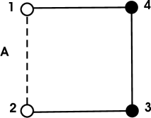
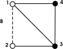
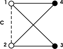
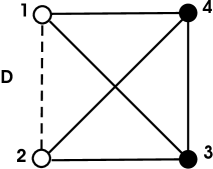
Figure 5: (A) Ring, (B) diagonal, (C) opened and (D) connected diagrams contributing to the ${\it E}_{4}$ component.

Explicit expressions of these components are,

$$E_{\rm 4R}={1\over 2}\frac{\rho^{3}}{\Omega}\int\prod_{1}^{4}d\mbox{\boldmath$r$}_{i}v^{*}(r_{12})f^{2}(r_{12})h(r_{23})h(r_{34})h(r_{41})\ ,$$ (33)

$$E_{\rm 4D}=2{1\over 2}\frac{\rho^{3}}{\Omega}\int\prod_{1}^{4}d\mbox{\boldmath$r$}_{i}v^{*}(r_{12})f^{2}(r_{12})h(r_{23})h(r_{34})h(r_{41})h(r_{24})\ ,$$ (34)

$$E_{\rm 4O}={1\over 2}{1\over 2}\frac{\rho^{3}}{\Omega}\int\prod_{1}^{4}d\mbox{\boldmath$r$}_{i}v^{*}(r_{12})f^{2}(r_{12})h(r_{23})h(r_{41})h(r_{24})h(r_{13})\ ,$$ (35)

$$E_{\rm 4C}={1\over 2}{1\over 2}\frac{\rho^{3}}{\Omega}\int\prod_{1}^{4}d\mbox{\boldmath$r$}_{i}v^{*}(r_{12})f^{2}(r_{12})h(r_{23})h(r_{34})h(r_{41})h(r_{24})h(r_{13})\ .$$ (36)

2.3.1 Calculation of $E_{\rm 4R}$ ring diagram

Figure 6: Density dependence of the ${\it E}_{\rm 4R}$ component for the AB potential.

It is easy to see that the ring diagram contribution to the energy is given by,

$$E_{\rm 4R}=\frac{1}{2}\rho^{3}\int\prod_{1}^{4}d\mbox{\boldmath$R$}_{i}f^{2}(R_{1})v^{*}(R_{1})h(R_{1})h(R_{2})h(R_{3})h(R_{4})\delta(\mbox{\boldmath$R$}_{1}+\mbox{\boldmath$R$}_{2}+\mbox{\boldmath$R$}_{3}+\mbox{\boldmath$R$}_{4})$$ (37)

or equivalently,

$$E_{\rm 4R} = \frac{1}{2}\rho^{3}\int\prod_{1}^{2}d\mbox{\boldmath$R$}_{i}f^{2}(R_{1})v^{*}(R_{1})h(R_{2})V_{h,h}^{\delta}(\mbox{\boldmath$R$}_{1}+\mbox{\boldmath$R$}_{2})$$ (38)

$$= \frac{1}{2}\rho^{3}\int\prod_{1}^{3}d\mbox{\boldmath$R$}_{i}f^{2}(R_{1})v^{*}(R_{1})h(R_{2})V_{h,h}^{\delta}(R_{3})\delta(\mbox{\boldmath$R$}_{3}-\mbox{\boldmath$R$}_{1}-\mbox{\boldmath$R$}_{2}),$$

in terms of the function $V_{h,h}^{\delta}$ defined in Eq.(29). In the hierarchy of $\delta$ kernel let us introduce,

$$V^{\delta\delta}_{p,q,r}(R_{1})=\int d\mbox{\boldmath$R$}_{2}d\mbox{\boldmath$R$}_{3}p(R_{2})V_{q,r}^{\delta}(R_{3})\delta(\mbox{\boldmath$R$}_{3}-\mbox{\boldmath$R$}_{1}-\mbox{\boldmath$R$}_{2})\ .$$ (39)

The final integral is simply,

$$E_{\rm 4R}={1\over 2}\rho^{3}\int d\mbox{\boldmath$R$}_{1}v^{*}(R_{1})f^{2}(R_{1})V^{\delta\delta}_{h,h,h}(R_{1})\ .$$ (40)

Using the expression for $V_{h,h}^{\delta}$ given in Eq.(30) we obtain the expression of $V^{\delta\delta}_{h,h,h}$,

$$V^{\delta\delta}_{h,h,h}(R) = \frac{\pi^{3}}{\beta^{6}}\left(\frac{1}{24\sqrt{3}}e^{-\frac{2}{3}R^{2}\beta^{2}}-\frac{3}{8\sqrt{2}}e^{-\frac{R^{2}\beta^{2}}{2}}\right.$$ (41)

$$+ \left.\frac{12}{5\sqrt{5}}e^{\frac{-2R^{2}\beta^{2}}{5}}-\frac{8}{3\sqrt{3}}e^{\frac{-R^{2}\beta^{2}}{3}}\right)\ .$$

The corresponding expression for $E_{\rm 4R}$ is:

$$E_{\rm 4R}=\frac{\pi^{9/2}\rho^{3}}{\beta^{6}}\left[\frac{c}{\beta}\left(\frac{3}{4}+\frac{3}{128\sqrt{2}}+\frac{7}{4\sqrt{3}}+\right.\right.$$

$$\left.\left.-\frac{12}{25\sqrt{5}}-\frac{240}{49\sqrt{7}}\right)+H_{R}V_{R}-H_{A}V_{A}\right]\ .$$ (42)

In the equation (42) the $H_{i}$’s are defined by

$$H_{i}=\frac{1}{16}\left(-6\chi_{1,2}(\beta,\mu_{i})+12\chi_{3,2}(\beta,\mu_{i})-6\chi_{5,2}(\beta,\mu_{i})-64\chi_{1,3}(\beta,\mu_{i})+\right.$$

$$\left.\chi_{2,3}(\beta,\mu_{i})+128\chi_{4,3}(\beta,\mu_{i})-2\chi_{5,3}(\beta,\mu_{i})-64\chi_{7,3}(\beta,\mu_{i})\right.$$

$$\left.+\chi_{8,3}(\beta,\mu_{i})+96\chi_{2,5}(\beta,\mu_{i})-192\chi_{7,5}(\beta,\mu_{i})+96\chi_{12,5}(\beta,\mu_{i})\right)\ ,$$

where $(i=A,R)$.

From the inspection of Fig.6 we infer that the ring contribution to the four-body energy has the same behavior as $E_{3}$ save for a factor -1.

2.3.2 Calculation of $E_{\rm 4D}$ diagonal diagram

In order to isolate the angular variables, we proceed as follows,

$$E_{\rm 4D} = 2{1\over 2}\frac{\rho^{3}}{\Omega}\int\prod_{1}^{4}d\mbox{\boldmath$r$}_{i}v^{*}(r_{12})f^{2}(r_{12})h(r_{23})h(r_{34})h(r_{41})h(r_{24})$$

$$E_{\rm 4D} = 2{1\over 2}\frac{\rho^{3}}{\Omega}\int\prod_{1}^{5}d\mbox{\boldmath$R$}_{i}\prod_{1}^{4}d\mbox{\boldmath$r$}_{i}v^{*}(R_{1})f^{2}(R_{1})h(R_{2})h(R_{3})h(R_{4})h(R_{5})$$ (43)

$$\times\delta(\mbox{\boldmath$R$}_{1}-\mbox{\boldmath$r$}_{1}+\mbox{\boldmath$r$}_{2})\delta(\mbox{\boldmath$R$}_{2}-\mbox{\boldmath$r$}_{2}+\mbox{\boldmath$r$}_{3})\delta(\mbox{\boldmath$R$}_{3}-\mbox{\boldmath$r$}_{3}+\mbox{\boldmath$r$}_{4})$$

$$\times\delta(\mbox{\boldmath$R$}_{4}-\mbox{\boldmath$r$}_{4}+\mbox{\boldmath$r$}_{1})\delta(\mbox{\boldmath$R$}_{5}-\mbox{\boldmath$r$}_{2}+\mbox{\boldmath$r$}_{4})\ .$$

Performing the same manipulations as above we obtain,

$$E_{\rm 4D}=2\cdot\frac{1}{2}\rho^{3}\int\prod_{1}^{5}d\mbox{\boldmath$R$}_{i}f^{2}(R_{1})v^{*}(R_{1})h(R_{2})h(R_{3})h(R_{4})h(R_{5})$$

$$\delta(\mbox{\boldmath$R$}_{5}+\mbox{\boldmath$R$}_{1}+\mbox{\boldmath$R$}_{4})\delta(\mbox{\boldmath$R$}_{5}-\mbox{\boldmath$R$}_{2}-\mbox{\boldmath$R$}_{3})\ .$$ (44)

We observe that variables $\mbox{\boldmath$R$}_{i},i=1,2,3,4$ are decoupled. It can be seen easily that:

$$E_{\rm 4D}=\rho^{3}\int d\mbox{\boldmath$R$}_{1}d\mbox{\boldmath$R$}_{4}d\mbox{\boldmath$R$}_{5}f^{2}(R_{1})v^{*}(R_{1})h(R_{4})h(R_{5})V^{\delta}_{h,h}(R_{5})\delta(\mbox{\boldmath$R$}_{5}+\mbox{\boldmath$R$}_{1}+\mbox{\boldmath$R$}_{4})\ .$$ (45)

Finally we have,

$$E_{\rm 4D}=\frac{\pi^{9/2}\rho^{3}}{288\beta^{6}}\left(\frac{c}{\beta}\left(\frac{27}{8}-\frac{26624\sqrt{3}-7344}{49\sqrt{7}}+\frac{2432\sqrt{6}-10368}{25\sqrt{5}}-\right.\right.$$

$$\left.\left.{\frac{945}{2\sqrt{2}}+74\sqrt{3}}-{\frac{15552}{121\sqrt{11}}+\frac{580608}{169\sqrt{13}}-\frac{442368}{361\sqrt{19}}}\right)+V_{R}D_{R}-V_{A}D_{A}\right)\ ,$$ (46)

Figure 7: Density dependence of the ${\it E}_{\rm 4D}$ component.

and the $D_{i}$’s are given by,

$$D_{i} = -9\left[\chi_{1,1}(\beta,\mu_{i})+\chi_{3,1}(\beta,\mu_{i})-2\chi_{2,1}(\beta,\mu_{i})-4(\chi_{6,5}(\beta,\mu_{i})+\chi_{16,5}(\beta,\mu_{i}))\right.$$ (47)

$$+8(\chi_{3,4}(\beta,\mu_{i})+\chi_{11,4}(\beta,\mu_{i})+\chi_{11,5}(\beta,\mu_{i}))$$

$$-16(\chi_{2,3}(\beta,\mu_{i})+\chi_{8,3}(\beta,\mu_{i})+\chi_{7,4}(\beta,\mu_{i}))$$

$$+2^{5}(\chi_{5,3}(\beta,\mu_{i})+\sqrt{2}(\chi_{22,7}(\beta,\mu_{i})+\sqrt{2}\chi_{8,7}(\beta,\mu_{i})))$$

$$-2^{6}\sqrt{2}\chi_{15,7}(\beta,\mu_{i})$$

$$-2^{7}(\chi_{10,9}(\beta,\mu_{i})+\chi_{28,9}(\beta,\mu_{i}))$$

$$+2^{8}(\chi_{6,7}(\beta,\mu_{i})+\chi_{5,7}(\beta,\mu_{i})+\chi_{19,9}(\beta,\mu_{i})+\chi_{19,7}(\beta,\mu_{i})+\chi_{20,7}(\beta,\mu_{i}))$$

$$-2^{8}(\chi_{8,11}(\beta,\mu_{i})+\chi_{10,11}(\beta,\mu_{i})+\chi_{30,11}(\beta,\mu_{i})+\chi_{32,11}(\beta,\mu_{i}))$$

$$+2^{9}(\chi_{5,8}(\beta,\mu_{i})+\chi_{21,8}(\beta,\mu_{i})+\chi_{19,11}(\beta,\mu_{i})+\chi_{21,11}(\beta,\mu_{i}))$$

$$-2^{9}(\chi_{3,5}(\beta,\mu_{i})+\chi_{13,5}(\beta,\mu_{i})+\chi_{12,7}(\beta,\mu_{i})+\chi_{13,7}(\beta,\mu_{i}))$$

$$\left.+2^{10}(\chi_{8,5}(\beta,\mu_{i})-\chi_{13,8}(\beta,\mu_{i}))\right]\ ,$$

where $(i=A,R)$.

2.3.3 Calculation of $E_{\rm 4O}$ open diagram

Performing the usual manipulations on the $E_{\rm 4O}$ term we obtain,

$$E_{\rm 4O} = \frac{1}{4}\rho^{3}\int\prod_{1}^{5}d\mbox{\boldmath$R$}_{i}f^{2}(R_{1})v^{*}(R_{1})h(R_{2})h(R_{3})h(R_{4})h(R_{5})$$ (48)

$$\delta(\mbox{\boldmath$R$}_{1}+\mbox{\boldmath$R$}_{3}+\mbox{\boldmath$R$}_{4})\delta(\mbox{\boldmath$R$}_{5}-\mbox{\boldmath$R$}_{1}-\mbox{\boldmath$R$}_{2})\ .$$

The latter equation is simply,

$$E_{\rm 4O}=\frac{1}{4}\rho^{3}\int d\mbox{\boldmath$R$}_{1}f^{2}(R_{1})v^{*}(R_{1}){[V_{h,h}^{\delta}(R_{1})]}^{2}\ ,$$ (49)

and after substitution of eq.(1),

$$E_{\rm 4O}=\frac{\pi^{9/2}\rho^{3}}{\beta^{6}}\left(\frac{c}{\beta}\left(-\frac{48}{19\sqrt{19}}+\frac{336}{169\sqrt{13}}+\frac{63-64\sqrt{3}}{294\sqrt{7}}+\right.\right.$$

$$\left.\left.\frac{20\sqrt{6}-27}{150\sqrt{5}}-\frac{3}{22\sqrt{11}}-\frac{177}{256\sqrt{2}}+\frac{3}{1024}+\frac{191\sqrt{3}}{576}\right)+P_{R}V_{R}-P_{A}V_{A}\right)$$ (50)

where,

$$P_{i} = \frac{1}{2}\chi_{1,1}(\beta,\mu_{i})-\frac{255}{256}\chi_{2,1}(\beta,\mu_{i})+\frac{63}{128}\chi_{3,1}(\beta,\mu_{i})$$

$$+\frac{1}{256}\chi_{4,1}(\beta,\mu_{i})+\frac{1}{4}\chi_{3,2}(\beta,\mu_{i})-\frac{1}{2}\chi_{5,2}(\beta,\mu_{i})$$

$$+\frac{1}{4}\chi_{7,2}(\beta,\mu_{i})+\frac{4}{3\sqrt{3}}\chi_{4,3}(\beta,\mu_{i})-\frac{1}{4}\chi_{5,3}(\beta,\mu_{i})$$

$$-\frac{8}{3\sqrt{3}}\chi_{7,3}(\beta,\mu_{i})+\frac{1}{2}\chi_{8,3}(\beta,\mu_{i})+\frac{4}{3\sqrt{3}}\chi_{10,3}(\beta,\mu_{i})$$

$$-\frac{1}{4}\chi_{11,3}(\beta,\mu_{i})-8\chi_{7,6}(\beta,\mu_{i})+16\chi_{13,6}(\beta,\mu_{i})$$

$$-8\chi_{19,6}(\beta,\mu_{i})$$

Figure 8: Density dependence of the ${\it E}_{\rm 4O}$ component.

The density dependence of the $E_{4O}$ component is displayed in Fig. 8.

2.3.4 Calculation of $E_{4C}$ connected diagram

In this subsection we estimate,

$$E_{\rm 4C}=\frac{1}{4}\frac{\rho^{3}}{\Omega}\int\prod_{1}^{4}d\mbox{\boldmath$r$}_{i}v^{*}(r_{12})f^{2}(r_{12})h(r_{23})h(r_{34})h(r_{41})h(r_{24})h(r_{13})\ .$$ (51)

Using the same technique as above we introduce $\delta$ kernels,

$$E_{\rm 4C}=\frac{1}{4}\rho^{3}\int\prod_{1}^{6}d\mbox{\boldmath$R$}_{i}v^{*}(R_{1})f^{2}(R_{1})h(R_{2})h(R_{3})h(R_{4})h(R_{5})h(R_{6})$$

$$\delta(\mbox{\boldmath$R$}_{6}+\mbox{\boldmath$R$}_{3}+\mbox{\boldmath$R$}_{4})\delta(\mbox{\boldmath$R$}_{5}-\mbox{\boldmath$R$}_{2}-\mbox{\boldmath$R$}_{3})\delta(\mbox{\boldmath$R$}_{6}-\mbox{\boldmath$R$}_{1}-\mbox{\boldmath$R$}_{2})\ .$$ (52)

The identities

$$(2\pi)^{3}\delta\left(\mbox{\boldmath$R_{6}$}+\mbox{\boldmath$R_{3}$}+\mbox{\boldmath$R_{4}$}\right)=\int d\mbox{\boldmath$q_{1}$}\exp(\mbox{\boldmath$q_{1}$}.(\mbox{\boldmath$R_{6}$}+\mbox{\boldmath$R_{3}$}+\mbox{\boldmath$R_{4}$}))\ ,$$ (53)

$$(2\pi)^{3}\delta\left(\mbox{\boldmath$R_{5}$}-\mbox{\boldmath$R_{2}$}-\mbox{\boldmath$R_{3}$}\right)=\int d\mbox{\boldmath$q_{2}$}\exp(\mbox{\boldmath$q_{2}$}.(\mbox{\boldmath$R_{5}$}-\mbox{\boldmath$R_{2}$}-\mbox{\boldmath$R_{3}$})),$$ (54)

$$(2\pi)^{3}\delta\left(\mbox{\boldmath$R_{6}$}-\mbox{\boldmath$R_{1}$}-\mbox{\boldmath$R_{2}$}\right)=\int d\mbox{\boldmath$q_{3}$}\exp(\mbox{\boldmath$q_{3}$}.(\mbox{\boldmath$R_{6}$}-\mbox{\boldmath$R_{1}$}-\mbox{\boldmath$R_{2}$}))\ ,$$ (55)

are introduced in Eq.(52). The latter equation is then expressed in terms of the Fourier transform of $h$, labelled $\widetilde{h}$ and that of $v^{*}f^{2}$, labelled $G$. More precisely,

$$E_{\rm 4C}=\frac{1}{2048\pi^{9}}\rho^{3}\int\prod_{i=1}^{3}d\mbox{\boldmath$q_{i}$}\ \widetilde{h}(\mbox{\boldmath$q_{1}$}-\mbox{\boldmath$q_{2}$})\widetilde{h}(\mbox{\boldmath$q_{1}$}+\mbox{\boldmath$q_{3}$})\widetilde{h}(\mbox{\boldmath$q_{2}$}+\mbox{\boldmath$q_{3}$})\widetilde{h}(\mbox{\boldmath$q_{1}$})\widetilde{h}(\mbox{\boldmath$q_{2}$})G(\mbox{\boldmath$q_{3}$})\ .$$ (56)

For the sake of simplicity use is made of the scaling $\mbox{\boldmath$q_{j}$}\mapsto 2\sqrt{2}\beta\mbox{\boldmath$q_{j}$}$ in Eq.(56) in order to eliminate the $\beta$ dependence in $\widetilde{h}$. Introducing,

$$h^{*}(\mbox{\boldmath$q$})=-2e^{-2q^{2}}+\frac{1}{2\sqrt{2}}e^{-q^{2}}\ ,$$ (57)

such that $\widetilde{h}(2\sqrt{2}\beta\mbox{\boldmath$q$})\equiv(\sqrt{\pi}/b)^{3}h^{*}(\mbox{\boldmath$q$})$, the equation (56) becomes,

$$E_{\rm 4C}=\frac{4\sqrt{2}\ }{\beta^{6}\sqrt{\pi}^{3}}\rho^{3}\int\prod_{i=1}^{3}d\mbox{\boldmath$q_{i}$}\ h^{*}(\mbox{\boldmath$q_{1}$}-\mbox{\boldmath$q_{2}$})h^{*}(\mbox{\boldmath$q_{1}$}+\mbox{\boldmath$q_{3}$})h^{*}(\mbox{\boldmath$q_{2}$}+\mbox{\boldmath$q_{3}$})$$

$$h^{*}(\mbox{\boldmath$q_{1}$})h^{*}(\mbox{\boldmath$q_{2}$})G(2\sqrt{2}\beta\mbox{\boldmath$q_{3}$})\ .$$ (58)

The auxiliary integral

$$J(\mbox{\boldmath$q_{3}$})=\int\prod_{i=1}^{2}d\mbox{\boldmath$q_{i}$}\ h^{*}(\mbox{\boldmath$q_{1}$}-\mbox{\boldmath$q_{2}$})h^{*}(\mbox{\boldmath$q_{1}$}+\mbox{\boldmath$q_{3}$})h^{*}(\mbox{\boldmath$q_{2}$}+\mbox{\boldmath$q_{3}$})h^{*}(\mbox{\boldmath$q_{1}$})h^{*}(\mbox{\boldmath$q_{2}$})\ ,$$ (59)

entering the definition of $E_{4c}$, has been performed by using the Cartesian coordinates. We obtain after calculations $J(\mbox{\boldmath$q_{3}$})=\pi^{3}\ Q(q_{3})$ with,

$$Q(q) = \frac{-9\ \sqrt{2}+2\ \sqrt{3}}{72}\ \exp(-2\ q^{2})+\frac{8}{13\ \sqrt{13}}\ \exp\left(-\frac{22}{13}\ q^{2}\right)$$ (60)

$$- \frac{4}{19\ \sqrt{19}}\ \exp\left(-\frac{32}{19}\ q^{2}\right)+\left(\frac{1}{56\ \sqrt{7}}-\frac{1}{20\ \sqrt{5}}\right)\exp\left(-\frac{3}{2}q^{2}\right)$$

$$- \frac{2}{21\ \sqrt{21}}\ \exp\left(-\frac{10}{7}q^{2}\right)+\frac{1}{30\ \sqrt{30}}\ \exp\left(-\frac{7}{5}q^{2}\right)$$

$$+ \left(\frac{1}{30\ \sqrt{30}}-\frac{2}{21\ \sqrt{21}}\right)\exp\left(-\frac{4}{3}\ q^{2}\right)+\frac{1}{64\ \sqrt{2}}\exp\left(-\frac{19}{16}\ q^{2}\right)$$

$$- \frac{1}{88\ \sqrt{11}}\exp\left(-\frac{13}{11}\ q^{2}\right)+\frac{9-16\ \sqrt{3}}{36864}\ \exp(-q^{2})\ .$$

Figure 9: Density dependence of the ${\it E}_{\rm 4C}$ component.

Therefore,

$$E_{\rm 4C}=\frac{4\sqrt{2}\sqrt{\pi}^{3}\ }{\beta^{6}\ }\rho^{3}\int\ d\mbox{\boldmath$q_{3}$}\ Q(q_{3})G(2\sqrt{2}\beta\mbox{\boldmath$q_{3}$})$$ (61)

is expressed in terms of the 3D Fourier transform ($G$) of $v^{*}(r)f^{2}(r)$, which is given by,

Figure 10: ${\it E}_{2},{\it E}_{3},{\it E}_{4},{\it E_{tot}}$ density dependence.

$$G(q) = \pi^{3/2}\ \left\{c\ \left[\frac{3}{\sqrt{2\ }\ \beta}\ \exp\left(-\frac{q^{2}}{8\ \beta^{2}}\right)-\frac{q^{2}}{\beta^{3}}\ \exp\left(-\frac{q^{2}}{4\ \beta^{2}}\right)\right]\right.$$

$$\left.+V_{R}\left[\frac{1}{4\ \mu_{R}^{3}}\exp\left(-\frac{q^{2}}{4\mu_{R}^{2}}\right)-\frac{2}{(\beta^{2}+\mu_{R}^{2}\ )^{3/2}}\exp\left(-\frac{q^{2}}{4\ (\beta^{2}+\mu_{R}^{2})}\right)\right.\right.$$

$$\left.\left.+\frac{1}{(2\ \beta^{2}+\mu_{R}^{2}\ )^{3/2}}\exp\left(-\frac{q^{2}}{4\ (2\ \beta^{2}+\mu_{R}^{2})}\right)\right]-V_{A}\left[\frac{1}{4\ \mu_{A}^{3}}\exp\left(-\frac{q^{2}}{4\mu_{A}^{2}}\right)\right.\right.$$

$$-\frac{2}{(\beta^{2}+\mu_{A}^{2}\ )^{3/2}}\exp\left(-\frac{q^{2}}{4\ (\beta^{2}+\mu_{A}^{2})}\right)$$

$$\left.\left.+\frac{1}{(2\ \beta^{2}+\mu_{A}^{2}\ )^{3/2}}\exp\left(-\frac{q^{2}}{4\ (2\ \beta^{2}+\mu_{A}^{2})}\right)\right]\right\}\ ,$$

we are left with the final expression of $E_{4C}$:

$$E_{\rm 4C} = \frac{4\sqrt{2}\ \pi^{9/2}}{\beta^{6}}\rho^{3}\left[\frac{c}{\beta}\left(-\frac{3142463}{276480000}-\frac{200\ \sqrt{2}}{867\ \sqrt{51}}+\frac{657\ \sqrt{2}}{1225\ \sqrt{35}}\right.\right.$$ (62)

$$+ \left.\left.\frac{239063}{2074464\ \sqrt{2}}-\frac{19}{64\ \sqrt{3}}+\frac{243}{2450\ \sqrt{35}}\right)+C_{R}V_{R}-C_{A}V_{A}\right]\ .$$

The latter equation is expressed in terms of the $C_{i}$’s, $i=A,R$ which are listed in the Appendix.

Figure 11: Total energy for the case of the Ali-Bodmer potential compared to the Gogny D1 and D1N

The contribution to the energy supplied by each component of the cluster expansion is summarized in Fig.10 for the AB interaction. Clearly the major contributions come from $E_{2}$ and $E_{3}$ whereas the four-body contributions are very weak. In contrast to two-body contributions the three-body and four-body contribution are repulsive and the equilibrium arises from a delicate balance between $E_{2}$ and $E_{3}$ components.

We display in Fig. 11 a comparison of the EOS determined using the Ali-Bodmer potential with EOS obtained using D1 and D1N parametrizations of the Gogny potential. More details are given in Fig. 12. While the equilibrium point predicted by the AB interaction is deep and lies at the normal nuclear matter density, Gogny parametrizations predict a shallower minimum at densities close to the Mott density.

Figure 12: ${\it E}_{2},{\it E}_{3},{\it E}_{4},{\it E}$ dependence of the $\alpha$-matter density $\rho$.(Ali-Bodmer and Gogny)

The four-body contribution to the total energy is small compared to other components. This is explained by an almost complete cancellation between $E_{4R}$ and $E_{4D}$ while the most connected diagrams $E_{4O}$ and $E_{4C}$ are intrinsically small due to increased number of bonds (see Fig. 13).

Figure 13: ${\it E}_{\rm 4R},{\it E}_{\rm 4D},{\it E}_{\rm 4O},{\it E}_{\rm 4C},{\it E}_{4}$ dependence of the $\alpha$-matter density $\rho$.(Ali-Bodmer and Gogny)

3 Concluding remarks

By assuming a simple but realistic functional form for the TBCFN’s and employing Gaussian-like potentials, we obtained analytical expressions for the first six terms (one corresponding to the two-body, one to the three-body and four for the four-body diagrams) occurring in the cluster expansion of an extended uniform system of structureless, indistinguishable $\alpha$ particles in a uniform background of neutralizing charge. The results are pointing to a saturation of the alpha matter at densities around the nuclear matter density (for Ali-Bodmer potential) and for the D1 interaction at almost one tenth of this density. We also demonstrated the strength of the folding method, previously applied in the calculation of the heavy-ion potential [12] to the calculation of cluster integrals of a many-boson system.

4 Appendix

In this section we report the coefficients $C_{i}$ entering the final expression of $E_{4C}$. They are given below in terms of the coefficients,

$$\chi_{mn}=\frac{1}{(m\beta^{2}+n\mu_{i}^{2})^{3/2}}\ .$$ (63)

We have,

$$C_{i} = \left(\frac{1}{24\ \sqrt{6}}-\frac{1}{16}\right)\ \chi_{1,1}(\beta,\mu_{i})+\left(\frac{513}{4096}-\frac{1}{768\ \sqrt{3}}-\frac{1}{12\ \sqrt{6}}\right)\ \chi_{2,1}(\beta,\mu_{i}))$$ (64)

$$+ \left(-\frac{129}{2048}+\frac{1}{384\ \sqrt{3}}+\frac{1}{24\ \sqrt{6}}\right)\ \chi_{3,1}(\beta,\mu_{i})$$

$$+ \left(\frac{1}{40\ \sqrt{5}}-\frac{1}{7\ \sqrt{14}}\right)\chi_{3,2}(\beta,\mu_{i})$$

$$+ \left(\frac{1}{4096}-\frac{1}{768\ \sqrt{3}}\right)\ \chi_{4,1}(\beta,\mu_{i})+\left(-\frac{1}{5\ \sqrt{10}}+\frac{1}{14\ \sqrt{14}}\right)\ \chi_{4,3}(\beta,\mu_{i})$$

$$+ \left(\frac{\sqrt{2}}{7\sqrt{7}}-\frac{1}{20\ \sqrt{5}}\right)\ \chi_{5,2}(\beta,\mu_{i})+\left(\frac{1}{40\ \sqrt{5}}-\frac{1}{7\ \sqrt{14}}\right)\ \chi_{7,2}(\beta,\mu_{i})$$

$$+ \left(\frac{\sqrt{2}}{5\ \sqrt{5}}-\frac{1}{7\ \sqrt{14}}\right)\ \chi_{7,3}(\beta,\mu_{i})-\frac{1}{3\ \sqrt{6}}\ \chi_{7,5}(\beta,\mu_{i})$$

$$+ \left(-\frac{1}{5\ \sqrt{10}}+\frac{1}{14\ \sqrt{14}}\right)\ \chi_{10,3}(\beta,\mu_{i})+\frac{1}{6\ \sqrt{6}}\ \chi_{10,7}(\beta,\mu_{i})$$

$$+ \frac{\sqrt{2}}{3\sqrt{3}}\ \chi_{12,5}(\beta,\mu_{i})+2\ \sqrt{2}\ \chi_{13,11}(\beta,\mu_{i})-\frac{1}{3\ \sqrt{6}}\chi_{17,5}(\beta,\mu_{i})$$

$$- \frac{1}{3\ \sqrt{6}}\ \chi_{17,7}(\beta,\mu_{i})-\sqrt{2}\ \chi_{19,16}(\beta,\mu_{i})-\frac{1}{8}\ \chi_{22,13}(\beta,\mu_{i})$$

$$+ \frac{1}{6\ \sqrt{6}}\ \chi_{24,7}(\beta,\mu_{i})-4\ \sqrt{2}\ \chi_{24,11}(\beta,\mu_{i})+\frac{1}{\sqrt{2}}\ \chi_{32,19}(\beta,\mu_{i})$$

$$+ 2\ \sqrt{2}\ \chi_{35,11}(\beta,\mu_{i})+\frac{1}{4}\ \chi_{35,13}(\beta,\mu_{i})+2\ \sqrt{2}\ \chi_{35,16}(\beta,\mu_{i})$$

$$- \frac{1}{8}\ \chi_{48,13}(\beta,\mu_{i})-\sqrt{2}\ \chi_{51,16}(\beta,\mu_{i})$$

$$- \sqrt{2}\ \chi_{51,19}(\beta,\mu_{i})+\frac{1}{\sqrt{2}}\ \chi_{70,19}(\beta,\mu_{i}).$$

where $(i=A,R)$.

Acknowledgements

We are indebted to Roland Lombard for reading the manuscript and for suggestions. This work was partly supported by CNCSIS Romania, under program PN-II-PCE-2007-1, contracts No.49 and No.258 and by CNMP contract PNCDI2 D7 7.4 No.71112.

References

• [1] J. M. Lattimer, F. Douglas Swesty, Nucl. Phys. A535 331 (1983).
• [2] G. Röpke and P. Schuck, Mod.Phys.Lett. A21 2513 (2006).
• [3] K. Schäfer and G. Schütte, Nucl. Phys. A183 1 (1972).
• [4] J. B. Aviles, Jr., Ann. Phys. (N.Y.) 5 251 (1958).
• [5] E. Feenberg, Theory of Quantum Fluids, Academic Press, New York, 1969.
• [6] S. Ali and A. R. Bodmer, Nucl. Phys. A80, 99 (1966).
• [7] B. Buck, H. Friedrich and C. Wheatley, Nucl. Phys. A275, 246 (1977).
• [8] J. Meyer, Interactions Effectives, Théorie de Champs Moyen, Masses et Rayons Nucléaires, Ann.Phys.Fr.28 (2003).
• [9] F.Carstoiu and Ş. Mişicu, Saturation and condensate fraction reduction of cold alpha matter, Phys. Lett. B682, 33(2009)
• [10] V. G. Neudatchin, V. I. Kukulin, V. L. Korotkikh and V. P. Korennoy, Phys. Lett. B34, 581 (1971).
• [11] J. W. Clark and Tso-Pin Wang , Ann. Phys. (N.Y.) 40, 127 (1966).
• [12] F. Carstoiu and R. J. Lombard, Ann. Phys. (N.Y.) 217, 279 (1992).