Local Empathy provides Global Minimization of Congestion in Communication Networks

Abstract

We present a novel mechanism to avoid congestion in complex networks based on a local knowledge of traffic conditions and the ability of routers to self-coordinate their dynamical behavior. In particular, routers make use of local information about traffic conditions to either reject or accept information packets from their neighbors. We show that when nodes are only aware of their own congestion state they self-organize into a hierarchical configuration that delays remarkably the onset of congestion although leading to a sharp first-order like congestion transition. We also consider the case when nodes are aware of the congestion state of their neighbors. In this case, we show that empathy between nodes is strongly beneficial to the overall performance of the system and it is possible to achieve larger values for the critical load together with a smooth, second-order like, transition. Finally, we show how local empathy minimize the impact of congestion as much as global minimization. Therefore, here we present an outstanding example of how local dynamical rules can optimize the system’s functioning up to the levels reached using global knowledge.

I Introduction

Complex communication networks have recently attracted a lot of attention from scientists due to the discovery of the topological features of real communication systems such as the Internet bookvesp . The structure of these communication systems is efficiently described by a graph in which nodes represent routers and edges account for the communication channels. However, the structure of these graphs is far from being purely random. Quite on the contrary, they typically show a scale-free (SF) distribution for the number of communication channels departing from and arriving to a system’s element. The use of modern complex network theory rev:albert ; rev:newman ; rev:bocc together with tools inherited from non-equilibrium statistical physics rev:doro2 have allowed to study the dynamical properties of such communication systems. In particular, this approach has been successfully applied to the study of the structural evolution str1 ; str2 of the Internet, its navigability nav1 ; nav2 ; nav3 and dynamical properties flow0 ; flow1 ; flow2 , or the design of an efficient Digital Immune System targ ; holme ; cohen ; cov1 ; cov2 ; chen .

A lot of the recent literature on communication networks has tackled the critical properties of their jamming and congestion transitions Ohira ; Sole1 ; Sole2 ; cong1 ; Guimera ; cong01 ; cong2 ; cong55 ; cong7 ; cong77 . These studies have focused on the design of efficient routing strategies that, on one hand, provide with short delivery times and, on the other hand, avoid the onset of the congested state in which the load of packets in the system increases, thus causing the failure of information flow. It has been shown that finding the best suited strategy depends strongly on two main features: the topological patterns of the particular network and the load of information on top of it. Regarding the first of these two issues, a number of routing mechanisms have been studied on different structures cong5 ; cong6 ; cong7 ; cong15 allowing to design resilient network backbones cong1114 ; cong14 ; cong114 .

Many of the routing policies proposed so far rely on the (static) structural properties of the communication network. Examples of such policies are biased random walks cong888 ; cong88 , shortest-path SP ; cong8 and efficient-path EP schemes. These routing mechanisms can be conveniently reformulated to incorporate the information about the dynamical state of the system, i.e. the congestion state of routers. This allows to dynamically change the paths followed by information packets in order to bypass those over-congested routes. In this line, congestion-aware schemes have significantly improved the performance of biased random walks DRW , shortest-path cong3 ; cong4 and efficient-path cong16 routings. In addition to the design of efficient routing protocols, several strategies to avoid congestion have been implemented. Remarkable examples of these strategies are the implementation of incoming flow rejection cong10 ; cong11 and packet-dropping mechanisms cong111 for avoiding the congestion of single nodes, or the addition of a router memory to avoid packets getting trapped between two adjacent nodes cong9 .

All the above studies have assumed that both network topology and the mechanisms to avoid congestion are static (i.e. neither topology nor the routing strategies change). However, this approach neglects that, even for the same graph, the optimal routing policy depends strongly on the state of congestion of the system cong3 ; cong4 ; cong10 ; cong11 ; cong12 ; cong13 . Therefore, in order to balance correctly the congestion in a communication system it seems appropriate to allow the elements (routers) to switch to the best suited strategy to avoid congestion given the instant traffic conditions. In this article, we propose an adaptive mechanism that allows nodes to choose their individual strategies instead of imposing a common policy. In this adaptive protocol routers exploit their local information about the congestion state of the system to decide whether to accept incoming packets. First, in section II, we introduce a minimal routing model without any adaptive mechanism that allows us to unveil the role of rejection when it is externally tuned. In section III we will consider that each router can adopt its own rejection strategy and make some analytical derivations about the optimal strategic configuration to avoid the congestion onset. In section IV we will implement our first adaptive mechanism and show that when nodes are allowed to dynamically adapt their own strategy, while only being aware of their own congestion state (myopic case), the onset of congestion is shifted to a larger critical load (with respect to the static algorithm introduced in section II). This improvement is due to the self-organization of the strategies of nodes into degree-correlated configurations. However, we will show that the delay of the onset of congestion comes together with a sharp, first-order like, transition that provides no dynamical signals about the onset of congestion. Finally, in section V we show that when nodes are aware of the congestion state of its nearest neighbors and empathize with them, it is possible to recover the former large critical load together with a smooth phase transition, avoiding the uncertain scenario of the myopic adaptive model. More importantly, we will show that tuning conveniently the degree of empathy between routers it is possible to recover, through a local mechanism, both the congestion levels and the rejection patterns provided by the global minimization introduced in section III.

II Minimal traffic model

Let us start by introducing the minimal traffic model in which the adaptive algorithm will be implemented below. In this model, we consider the transfer of information packets between adjacent routers as a probabilistic event. Inspired by cong10 ; cong11 , we consider a set of stochastic equations for describing the time evolution of the queue length of the nodes at some time $t$, ${\bf q^{t}}=\{q_{i}^{t}\}$. The queue length of a given node, $q_{i}^{t}$, can either increase or decrease due to several events. First, at each time step and with probability $p$, a new packet is generated being added to the queue of the node. Second, at each time step each node tries to send a packet in its queue to any of its first neighbors. This packet can be rejected by the chosen neighbor with some probability $\eta$. If the packet is accepted, it may be removed from the system with certain probability $\mu$. These two latter events mimic the effects, although with some important differences, of an active queue control strategy as the random early detection (RED) Floyd1 present on Internet routers and the arrival of the packet to its final destination respectively. Following the above ingredients we can write the time-discrete Markov chain of the minimal traffic model as:

$$q_{i}^{t+1}=q_{i}^{t}+p + \sum_{j=1}^{N}\frac{\Theta(q_{j}^{t})A_{ji}}{k_{j}}(1-\mu)(1-\eta)$$ (1)

$$- \Theta(q_{i}^{t})\sum_{j=1}^{N}\frac{A_{ij}}{k_{i}}(1-\eta)\;,$$

where $A_{ij}$ represents the ($i$, $j$) term of the adjacency matrix of the network substrate and $\Theta(x)$ is the Heaviside step function ($\Theta(x)=1$ if $x>0$ and $\Theta(x)=0$ otherwise). Since our network is undirected and unweighted, the adjacency matrix is defined as $A_{ij}=A_{ji}=1$ if nodes $i$ and $j$ are connected and $A_{ij}=A_{ji}=0$ otherwise. The quantity $k_{i}$ is the degree of a node $i$ ($\sum_{j}A_{ij}=k_{i}$), i.e. the number of routers connected to it. The right-hand-side of equation (1) contains two terms accounting for the incoming flow of packets that arrive to the queue of node $i$, namely, $p$ (accounting for the external load of packets) and the first sum (accounting for the arrival of packets from its first neighbors). On the other hand, the second sum in equation (1) accounts for the probability that a packet from $i$ is delivered to a first neighbor.

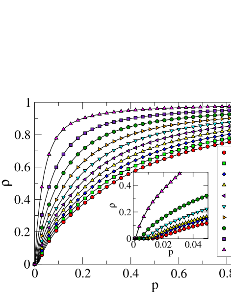
Figure 1: (Color online). Phase diagrams, $\rho(p)$, of the minimal traffic model using different values of the rejection rate $\eta$. The inset shows the existence of different critical values $p_{c}$ when varying $\eta$

The set of equations (1) are solved starting from a zero congestion state: $q_{i}^{0}=0$ $\forall i$. The evolution of the system is monitored by means of the following order parameter cong1 :

$$\rho(t)=\lim_{T\rightarrow\infty}\frac{Q(t+T)-Q(t)}{pT}\;,$$ (2)

where $Q(t)$ is the sum of all the queue lengths at time step $t$, $Q(t)=\sum_{i=1}^{N}q_{i}^{t}$. The stationary value, $\rho$, of the above order parameter is bounded ($0\leq\rho\leq 1$) and describes the dynamical regime in which the system ends up. Namely, $\rho=0$ indicates that the system is able to balance the incoming flow of new packets with a successful delivery of the old ones. In this case the system is said to operate in the free-flow regime. Instead, when $\rho>0$ the above balance is not fulfilled and the queues of the nodes increase their size in time at a rate $\rho\cdot p$. In this latter situation the system is in the congested phase.

We have studied the behavior of the order parameter $\rho$ by taking the rate of packet creation $p$ as the control parameter. The arrival-to-destination probability is set to $\mu=0.2$ as the usual value found in the Internet bookvesp . The corresponding phase diagrams are shown in Fig. 1 for several values of the rejection probability $\eta$ using a SF network of $N=5000$ with $P(k)\sim k^{-2.2}$. As observed in the figure, the transition from free-flow to congestion occurs in a smooth way at low values of $p$ being the critical point $p_{c}=0.02$ for $\eta=0$ (no rejection). However, as the rejection rate $\eta$ increases the value of $p_{c}$ decreases and $\rho$ increases faster (see inset in Fig. 1).

III Analytical approximation of global congestion minimization

The above results question the convenience of implementing a rejection mechanism in routing models. However, the bad performance of this rejection mechanism relies on the homogeneous distribution of the rejection rates across the routers of the network. We now explore the general situation in which the individual rejection rates are independent. Therefore the set of equations (1) transforms into:

$$q_{i}^{t+1}=q_{i}^{t}+p + \sum_{j=1}^{N}\frac{\Theta(q_{j}^{t})A_{ji}}{k_{j}}(1-\mu)(1-\eta_{i})$$ (3)

$$- \Theta(q_{i}^{t})\sum_{j=1}^{N}\frac{A_{ij}}{k_{i}}(1-\eta_{j})\;.$$

This new set of equations is now used to determine the optimal set $\{\eta_{i}\}$ so that congestion is minimized for a given value of $p$. To this aim, we first use two assumptions: (i) the nodes have reached a stationary state, $q_{i}^{t+1}=q_{i}^{t}$ $\forall i$, and (ii) the queue length of nodes is nonzero, $\Theta(q_{i}^{t})=1$ $\forall i$. These provisos admitted, equations (3) turn into the following set of equations for the rejection rates of the routers $\{\eta_{i}\}$:

$$0=p+\sum_{j=1}^{N}\frac{A_{ji}}{k_{j}}(1-\mu)(1-\eta)-\sum_{j=1}^{N}\frac{A_{ij}}{k_{i}}(1-\eta)\;.$$ (4)

Now we make use of the annealed approximation of the adjacency matrix Bianconi1 ; Bianconi2 ; Guerra :

$$A_{ij}=A_{ji}=\frac{k_{i}k_{j}}{N\langle k\rangle}\;,$$ (5)

where $\langle k\rangle$ is the average degree of the network ($\langle k\rangle\simeq 4$ in our case). Introducing the annealed expression (5) into equations (4) we obtain:

$$k_{i}(1-\eta_{i})=\frac{1}{1-\mu}\left[\langle k(1-\eta)\rangle-p\langle k\rangle\right]\;,$$ (6)

where $\langle k(1-\eta)\rangle=\sum_{j}k_{j}(1-\eta_{j})/N$. Equation (6) clearly shows that the larger the degree of a router the larger its rejection rate. Therefore, from this expression we observe that a non-homogeneous distribution of rejection rates across the routers is beneficial to assure the free-flow condition (and thus to delay the onset of congestion). We can calculate the expression of the rejection rate by computing the value of $\langle k(1-\eta)\rangle$. From equation (6) we obtain:

$$\langle k(1-\eta)\rangle=\frac{1}{1-\mu}\left[\langle k(1-\eta)\rangle-p\langle k\rangle\right]\;,$$ (7)

and finally we have:

$$\langle k(1-\eta)\rangle=\frac{p}{\mu}\langle k\rangle\;.$$ (8)

Therefore, the rejection rate of a node with connectivity $k_{i}$ reads:

$$\eta_{i}=1-\frac{p\langle k\rangle}{\mu k_{i}}\;.$$ (9)

As anticipated above, expression (9) shows that the rejection rates of nodes should depend on their degrees rather than being externally set to a constant value. In Fig. 2 we apply equation (9) to plot the rejection patterns corresponding to different values of the external load $p$. As shown, $\eta_{i}$ decreases with $p$ and increases with $k_{i}$.

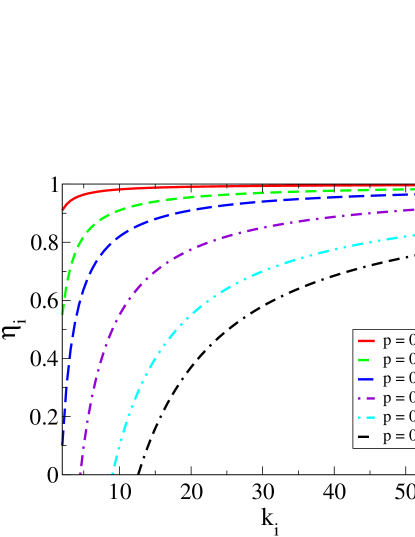
Figure 2: (Color online). Rejection rates of nodes as a function of their degree $\eta_{i}(k_{i})$ as obtained from equation (9). The curves correspond to different values of the external load of information $p$.

The assumptions made in order to obtain equation (9) point out that its validity, for all the nodes, should be restricted to the proximity of the critical point $p_{c}$. First, for $p<p_{c}$ many of the queues are zero (invalidating assumption (ii)) thus making the rejection rate imposed by equation (9) too restrictive for the real traffic conditions. On the other hand, for $p>p_{c}$ assumption (i) does not hold for all the nodes. This is manifested by the prediction of negative rejection rates, $\eta_{i}<0$, in equation (9) for those nodes with low connectivity. In practice, the impossibility of displaying negative rejection rates fixes their rejection rate to $\eta_{i}=0$. However, those nodes with large enough connectivity can still avoid congestion by means of positive rejection rates as described in equation (9) (see Fig. 2). Following these arguments, we can estimate the exact value of $p_{c}$ as the maximum value of $p$ for which $\eta_{i}\geq 0$ for all the nodes in the network. In particular, given that, for a given $p$, the value of $\eta_{i}$ increases with $k_{i}$ we obtain $p_{c}$ imposing in equation (9) that those nodes with the minimum connectivity, $k_{i}=k_{min}$, have $\eta_{i}=0$. Since in our case $k_{min}=2$ and $\langle k\rangle\simeq 4$ we obtain $p_{c}\simeq 0.1$. Therefore, by externally fixing the rejection rate of each node as dictated by equation (9) we can assure the permanence in the free-flow phase up to $p_{c}\simeq 0.1$.

IV Myopic adaptability

The minimal traffic model introduced in section II shows that system’s performance deteriorates as soon as rejection rates are uniformly set in the system. However, in section III we have shown that a non-uniform configuration for the rejection rates shifts the critical load to larger values. However, this non-uniform configuration has been externally imposed and derived analytically following different assumptions. A correct derivation of the optimal configuration would imply, on one hand, a more sophisticated calculation and, on the other hand, a complete knowledge of the architecture of the network. This latter condition makes unfeasible the external tuning of the individual rejection rates.

In order to overcome the need of global knowledge about the topology of the network we now introduce an adaptive scheme based solely on the local information available to nodes. In this adaptive setting we will allow nodes to choose their own rejection rate so that the dynamical state of a node will be described by both $q_{i}^{t}$ and $\eta_{i}^{t}$:

$$q_{i}^{t+1}=q_{i}^{t} + p+\sum_{j=1}^{N}\frac{\Theta(q_{j}^{t})A_{ji}}{k_{j}}(1-\mu)\left[1-\eta_{i}^{t}\right]$$ (10)

$$- \Theta(q_{i}^{t})\sum_{j=1}^{N}\frac{A_{ij}}{k_{i}}\left[1-\eta_{j}^{t}\right]$$

The individual choice of each instant value $\eta_{i}^{t}$ aims at operating at the optimal regime as given by the external parameters $p$ and $\mu$. To this aim, each node chooses its own rejection rate for the following time-step attempting to reach an optimal queue length, $q^{opt}=p/\mu$, so that traffic is homogeneously distributed across the network. To this end, a node raises or decreases its own rejection rate depending on the deviation of its instant queue length from the optimal queue, $\Delta_{i}^{t}=q_{i}^{t}-q^{opt}$. This rationale mimics a myopic behavior by which, regardless of the congestion state of the system, nodes are allowed to close the door to new packets while decreasing their respective queues. To incorporate this adaptive behavior we couple equations (10) with the following evolution equations for the set $\{\eta_{i}^{t}\}$:

$$\eta_{i}^{t+1}=\frac{1}{1+\exp{\left(-\beta\Delta_{i}^{t}\right)}}\;.$$ (11)

This evolution rule takes the form of the saturated Fermi function so that congested nodes, $q_{i}>q^{opt}$, will tend to total rejection, $\eta_{i}^{t+1}\rightarrow 1$, whereas those under-congested will open the door to new packets, $\eta_{i}^{t+1}\rightarrow 0$. The velocity of the transition from these two regimes is controlled by $\beta$ since it accounts for the reactivity of nodes to congestion. Note, that $\eta^{t+1}_{i}=0.5$ will be adopted whenever $q^{t}_{i}=q^{opt}$.

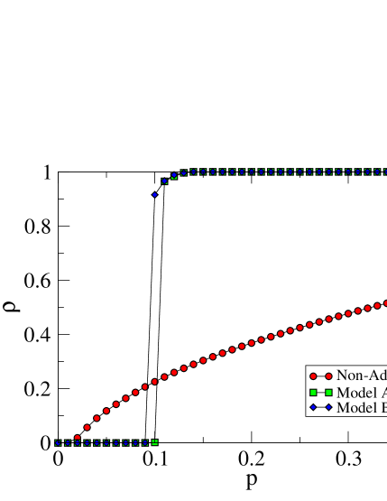
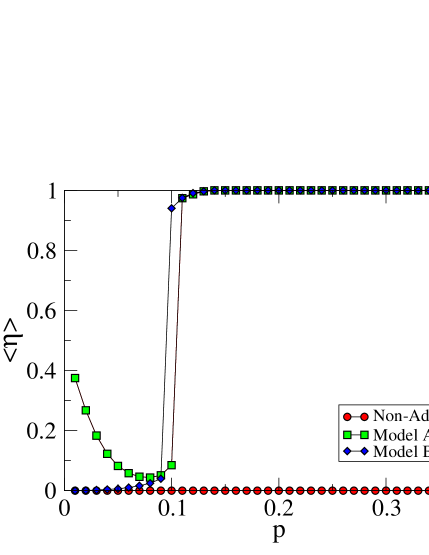
Figure 3: (Color online). (Top) Phase diagram $\rho(p)$ for the myopic routing models A (squares) and B (diamonds) and for the minimal routing model (circles). (Bottom) Average rejection rate $\langle\eta\rangle$ as a function of $p$ of the former three routing schemes.

The adaptive equations (11) allow for abrupt changes in the rejection rates between two consecutive time steps. Thus, we also explore a different formulation:

$$\eta_{i}^{t+1}=\eta_{i}^{t}+\beta\Delta_{i}^{t}\;,$$ (12)

in which the rejection rates evolve smoothly. Rule (12) is completed by assuring that $\eta_{i}$ remains bounded so that $0\leq\eta_{i}\leq 1$. In the above equation (12), $\beta$ acts as the inverse of the time between two consecutive time steps of the adaptive dynamics. Therefore, in the continuous time approximation of equation (12), the derivative of the rejection rate is equal to the difference between the instant queue length and its optimal value, i.e. $\Delta_{i}^{t}=q_{i}^{t}-q^{opt}$. Note that in this setting when $q^{t}_{i}=q^{opt}$ a router will adopt $\eta_{i}^{t+1}=0$.

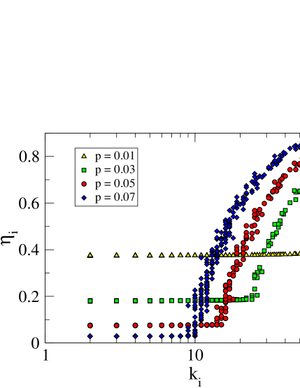
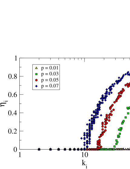
Figure 4: (Color online). Distribution of the individual rejection rates $\eta_{i}$ across degree-classes for several values of $p$ in the myopic routing models A (top) and B (bottom).

In the following we will use the two formulations for the myopic adaptive model and show that the results are qualitatively the same. Namely, we will call model A to equations (10) and (11), and model B to the formulation using equations (10) and (12). Note that in both models the parameter $\beta$ controls the reaction speed of nodes to congestion. In this direction, our numerics have shown that by changing $\beta$ one basically controls the duration of the transient time before the stationary distribution of the rejection rates is reached. In the following, we set $\beta=10$ and $\beta=10^{-2}$ in models A and B respectively.

In the top panel of Fig. 3 we show the phase diagram, $\rho(p)$, of the myopic adaptive model with the two formulations. As observed, in both formulations the myopic model displays an abrupt, first-order like, transition from the free-flow to the congested state. Moreover, in Fig. 3 we have also plotted the phase diagram of the minimal model when $\eta=0$, i.e. its most congestion-resilient version, to show the improvement of myopic adaptability by shifting the jamming transition from $p_{c}=0.02$ to $p_{c}\simeq 0.1$. This value for the critical load is exactly the same as the one predicted in section III by means of the analytical approximation using global knowledge. Thus, the myopic adaptive model, equals the delay of the congestion onset obtained by minimizing congestion globally.

To analyze the roots of the resilience of the myopic adaptive routing to congestion we have plotted in the bottom panel of Fig. 3 the mean value of the rejection rate, $\langle\eta\rangle=\sum_{i=1}^{N}\eta_{i}$. In this case we observe that models A and B display the same pattern after the sharp transition to congestion, i.e. the sudden closing of all the doors in the network thus causing the abrupt transition to $\rho\simeq 1$ as soon as $p>p_{c}$. On the other hand, the configurations adopted by both models before the onset of congestion, $p<p_{c}$, are quite different: While in model B $\langle\eta\rangle\simeq 0$, for model A a significant part of the population adopts $\eta_{i}>0$. Surprisingly, in this latter setting the average rejection rate decreases as we approach the critical point, $p_{c}$.

To have a deeper insight about the microscopic configurations that allow to delay the onset of congestion we show in Fig. 4 the set of individual rejection rates of nodes $\{\eta_{i}\}$ ranked according to their degrees. In both models A and B, the correlation between $\eta_{i}$ and $k_{i}$ is clear since all the routers within the same degree-class display similar rejection rates. First, in model A we observe that for $p=0.01$ the system self-organizes homogeneously around $\eta\simeq 0.4$. However, when $p$ increases the rejection rates of low-degree classes decreases while hubs start to close their doors progressively as $p$ increases. For model B the microscopic configurations adopted as $p$ increases are similar regarding the behavior of high-degree nodes. However, in this latter scenario low-degree nodes remain accepting incoming packets up to the congested state. These two figures show that the two different internal dynamics (showing different microscopic organizations ) lead to the same macroscopic result: the delay of the onset of congestion.

Let us highlight that the delay of the congestion onset in this myopic adaptive setting again contradicts the results obtained for the minimal routing model in which, even a small (homogeneously distributed across routers) rejection rate leads to an increase of the congestion in the system. Quite on the contrary, the myopic adaptive model points out the same idea concluded from the global minimization of congestion: a hierarchical (degree-based) organization of the rejection rates by the system is strongly beneficial to avoid the congestion of the system. However, from figure 4 it becomes evident that the strategies self-adopted in the myopic adaptive settings are clearly different than the ones obtained in section III from equation (9) when congestion was minimized using global knowledge. Although in equation (9) the value of the rejection rate increases with the degree of the node (as in the myopic setting), the evolution with $p$ is quite different. Thus, although the critical load has been shifted to the same value as the one found in section III, the self-organized patterns of the rejection rates in the myopic settings reveal a clearly different scenario.

V Empathetic adaptability

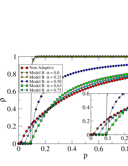
Figure 5: (Color online). (Top) Phase diagram $\rho(p)$ of the empathetic routing model for several values of the empathy parameter $\alpha$. The phase diagram of the minimal routing model (circles) is also plotted for the sake of comparison. (Bottom) For the same empathy parameters we show the average rejection rate $\langle\eta\rangle$ as a function of $p$. The function $\langle eta\rangle(p)$ obtained analytically from global minimization and computed from equation (9) is also shown.

The myopic adaptive setting has improved remarkably the resilience to congestion without the need of tuning any external parameters. However, the existence of an abrupt phase transition, again as found in cong3 ; cong4 ; cong8 ; cong9 , demands for further improvements. The main goal in order to soften such abrupt transition is to avoid that all the nodes close their doors due to its own congestion by incorporating an empathetic behavior based on the local knowledge about the dynamical state of their neighbors. This empathetic behavior should motivate congested nodes to open their doors when detecting an hyper-congested state in its surroundings. To this aim we take model B note and reformulate its equations as follows:

$$\eta_{i}^{t+1}=\eta_{i}^{t}+\beta\left[(1-\alpha)\Delta_{i}^{t}-\alpha\langle\Delta_{j}^{t}\rangle_{\Gamma_{i}}\right]\;.$$ (13)

In the above equations we introduce a new term accounting for the average level of congestion in the neighborhood, $\Gamma_{i}$, of a node $i$,

$$\langle\Delta_{j}^{t}\rangle_{\Gamma_{i}}=\sum_{j=1}^{N}\frac{A_{ij}}{k_{i}}\Delta_{j}^{t}\;.$$ (14)

The relative importance that nodes assign to the local level of congestion in their neighborhoods with respect to their own state is controlled by the parameter $\alpha$. In particular, when $\alpha=0$ we recover the myopic setting whereas for $\alpha=1$ routers behave “altruistically” and their decisions are based solely on their neighbor’s state of congestion. Thus, the parameter $\alpha$ measures the degree of empathy between connected routers.

In the top panel of Fig. 5 we plot the phase diagrams for several values of $\alpha$ together with that of the minimal non-adaptive routing model. We observe that for $\alpha<0.5$ the phase-transition is similar to that of the myopic adaptive model ($\alpha=0$), i.e. showing a critical load of $p_{c}\simeq 0.1$ followed by a first-order transition to full congestion. However, from the figure we observe that when $\alpha>0.5$ the transition to congestion occurs smoothly, thus recovering the behavior of the minimal model. On the other hand, the value of $p_{c}$ also decreases with $\alpha$ (thus anticipating the onset of congestion) although it remains close to the original value $p\simeq 0.1$ until $\alpha\simeq 0.63$. Moreover, for $p>p_{c}$, the curves corresponding to $\alpha=0.63$ and $\alpha=0.75$ reach levels of congestion similar to those observed in the minimal model.

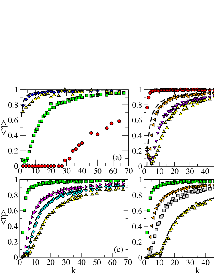
Figure 6: (Color online). Distribution of the mean rejection rates $\langle\eta\rangle$ across degree-classes of the empathetic adaptive model for several values of the empathy parameter $\alpha$ compared with the global minimization prediction (dashed line). Different traffic values $p$ are presented: (a) $p=0.02$ (free-flow regime), (b) $p=0.1$ (critical point), (c) $p=0.3$ and (d) $p=0.6$ (congested state)

In order to gain more insight about the strategy adopted in the empathetic setting we have computed the average level of rejection rate as a function of $p$ for the relevant values of $\alpha$. In the bottom panel of Fig. 5 we observe that those curves corresponding to $\alpha>0.5$ are quite different from those obtained in Fig. 3 for the myopic adaptive setting. In particular, when $p\ll p_{c}$ the empathetic adaptability shows a large amount of rejection. However, as $p$ increases the average rejection rate decreases monotonously. This high-rejecting behavior for $p<p_{c}$, was not observed in the myopic scheme. Quite on the contrary, it was shown that nearly all the doors were open in the sub-critical regime. However, the high rate of rejection observed in Fig. 5 is due to the large degree of empathy ($\alpha>0.5$) and the existence of a number of under-congested nodes, $\Delta_{i}<0$, in the sub-critical regime. Under these low traffic conditions, most nodes will close partially their doors when detecting under-congested neighborhoods, $\langle\Delta_{j}^{t}\rangle_{\Gamma_{i}}<0$, in order to benefit from the availability of neighbors to handle their packets. This situation is highly dynamical and most of the nodes experiment large fluctuations in their rejection rates until the system equilibrium is reached. This microscopic scenario, although clearly different from that of the myopic setting, enables to delay the onset of congestion in an efficient way. On the other hand, as $p$ approaches $p_{c}$ and for $p>p_{c}$ we observe that (for $\alpha>0.5$) the value of $\langle\eta\rangle$ decreases to $0$ as $p$ increases. This is due to both the large number of over-congested neighborhoods, $\langle\Delta_{j}^{t}\rangle_{\Gamma_{i}}>0$, surrounding routers in the super-critical regime and their large degree of empathy. As expected, empathy prevents from the sudden door closing when $p>p_{c}$, thus favoring a smooth phase transition displaying congestion levels simlar to those observed in the minimal routing model in the super-critical regime.

Interestingly, the monotonous decrease of $\langle\eta\rangle(p)$ from $\langle\eta\rangle=1$ at $p=0$ shown in Fig. 5, points out a similar behavior to that obtained by means of global minimization of congestion. As shown in the bottom panel of Fig. 5 the theoretical estimation of $\langle\eta\rangle(p)$ (circles) follows the same trend as the self-adopted patterns for $\alpha>0.5$. To analyze in detail the similarity between the empathetic setting and the microscopic patterns predicted by global minimization of congestion we plot in Fig. 6 the average value of the rejection rate as a function of the degree $k$ of the nodes, $\langle\eta\rangle(k)$, for several values of $p$ and $\alpha$. The panels correspond to (a) $p=0.02$ (free-flow regime), (b) $p=0.1$ (critical point), (c) $p=0.3$ and (d) $p=0.6$ (congested state). The shape of each curve $\langle\eta\rangle(k)$ behaves similarly to the theoretical one as predicted from equation (9). More importantly, for each value of $p$ there is one value of $\alpha$, $\alpha^{opt}$, for which the curve $\langle\eta\rangle(k)$ fits perfectly the prediction made by global minimization of congestion. The precise value of $\alpha^{opt}$ depends on $p$. In particular, for $p=0.02$ we find $\alpha^{opt}\simeq 0.63$, for $p=0.1$ we obtain $\alpha^{opt}\simeq 0.55$, for $p=0.3$ we have $\alpha^{opt}\simeq 0.68$ and, finally, for $p=0.6$ the value found is $\alpha^{opt}\simeq 0.75$. Moreover, from the top panel of Fig. 5, we observe that the values found for $\alpha^{opt}$ are those for which congestion, $\rho(p)$, is minimum. This result points out that empathetic adaptability is able to avoid congestion by means of only local information as much as global minimization does.

VI Conclusions

We have studied a novel mechanism that allows routers to adapt their individual strategies based on their local knowledge about congestion. Although in our approach nodes can only decide either to refuse or to accept incoming packets from their first neighbors, we obtain a variety of dynamical behaviors. First, we have analyzed the situation when no individual adaptability is allowed. This allows us to show that whenever a small level of rejection is applied indistinctly to all the nodes, one obtains a worse overall behavior than when all incoming flows are accepted by the routers. Then, we have considered that routers can have different rejection rates and derived analytically their patterns to minimize congestion, considering global knowledge of the network topology. With these globally optimized patterns the resilience to congestion of the system can be enhanced significantly. Besides, these patterns reveal a dependence of the rejection rate and the degree of the router while its mean value decays with the incoming load of packets.

After deriving global minimization of congestion we have studied the situation in which nodes self-adjust their own rejection rates dynamically depending on their instant level of congestion (myopic setting). In this case we have shown that the critical load of the network is shifted to a value similar to that found analytically by means of global minimization of congestion. This improvement is again achieved by a proper distribution of the rejection rates according to the degrees of the routers. However, in the adaptive case, such degree-correlated configuration is self-tuned by the system and differs from that obtained analytically. As usual in congestion-aware routing schemes, such delay in the congestion onset comes together with an abrupt transition from the free-flow phase to the congested one that prevents from having any warnings of the approach to the onset of congestion. For this reason, we have finally explored the situation in which routers also consider the congestion state of their first neighbors to adapt their rejection rates. We have shown that when nodes empathize with the congestion state of their neighbors, thus not rejecting packets from them when they detect an over-congested neighborhood, the shift in the critical load (obtained through global minimization and the myopic adaptability) is preserved and followed by a smooth congestion transition. Moreover, the analysis of the microscopic patterns of rejection rates when empathy is the mechanism at work points out a similar organization to that obtained from global minimization. In particular, it is possible to find the degree of empathy that perfectly agrees with the analytical estimation of the rejection pattern that minimize congestion for a given load of information.

In summary, we have shown that allowing routers to adapt their own strategies together with a certain degree of local empathy is strongly beneficial to the behavior of complex communication systems. Moreover, the improvement shown when local empathy is at work is similar to that obtained by minimizing congestion by means of a global knowledge of the network topology. Thus, the empathetic setting represents, a remarkable example of how local rules can achieve levels of functioning as optimal as those obtained with global knowledge of the system. Besides, our results open the relevant question about how local empathy can be naturally tuned as a function of the external inputs.

- (1) R. Pastor-Satorras and A. Vespignani, Evolution and Structure of the Internet: A Statistical Physics Approach, (Cambridge University Press, Cambridge, 2004).
- (2) R. Albert and A.-L. Barabási, Rev. Mod. Phys. 74, 47 (2002).
- (3) M.E.J. Newman, SIAM Review 45, 167 (2003).
- (4) S. Boccaletti, V. Latora, Y. Moreno, M. Chavez and D.-U. Hwang, Phys. Rep. 424, 175 (2006).
- (5) S.N. Dorogovtsev, A.V. Goltsev, and J.F.F. Mendes, Rev Mod. Phys. 80, 1275 (2008).
- (6) R. Pastor-Satorras, A. Vázquez, and A. Vespignani, Phys. Rev. Lett. 87, 258701 (2001).
- (7) M.A. Serrano, M. Boguñá, and A. Díaz-Guilera, Phys. Rev. Lett. 94, 038701 (2005).
- (8) M. Boguñá, D. Krioukov, Phys. Rev. Lett. 102, 058701 (2009).
- (9) M. Boguñá, D. Krioukov, and K.C. Claffy, Nature Phys. 5, 74 (2009).
- (10) C. Caretta Cartozo and P. De Los Rios, Phys. Rev. Lett. 102, 238703 (2009).
- (11) M. Argollo de Menezes, and A. L. Barabási, Phys. Rev. Lett. 92, 028701 (2004).
- (12) J. Duch, and A. Arenas, Phys. Rev. Lett. 96, 218702 (2006).
- (13) S. Meloni, J. Gómez-Gardeñes, V. Latora, and Y. Moreno, Phys. Rev. Lett. 100, 208701 (2008).
- (14) R. Pastor-Satorras, and A. Vespignani, Phys. Rev. E 65, 036104 (2002).
- (15) R. Cohen, S. Havlin, and D. ben-Avraham, Phys. Rev. Lett. 91, 247901 (2003).
- (16) P. Holme, EPL 68, 908 (2004).
- (17) P. Echenique, J. Gómez-Gardeñes, Y. Moreno, and A. Vázquez, Phys. Rev. E 71, 035102(R) (2005).
- (18) J. Gómez-Gardeñes, P. Echenique, and Y. Moreno, Eur. Phys. J. B 49, 259 (2006).
- (19) Y. Chen, G. Paul, S. Havlin, F. Liljeros, and H. E. Stanley, Phys. Rev. Lett. 101, 058701 (2008).
- (20) T. Ohira, and R. Sawatari, Phys. Rev. E 58, 193 (1998).
- (21) R. V. Solé, and S. Valverde, Physica A 289, 595 (2001).
- (22) S. Valverde and R. V. Solé, Physica A 312, 636 (2002).
- (23) R. Guimerá, A. Díaz-Guilera, F. Vega-Redondo, A. Cabrales, and A. Arenas, Phys. Rev. Lett. 89, 248701 (2002).
- (24) R. Guimerá, A. Arenas, A. Díaz-Guilera, and F. Giralt, Phys. Rev. E 66, 026704 (2002).
- (25) B. Tadic and G.J. Rodgers, Adv. Complex Systems 5, 445 (2002).
- (26) Z. Toroczkai, and K. E. Bassler, Nature 428, 716 (2004).
- (27) B. Kujawski, J.G. Rodgers, and B. Tadic, Lecture Notes in Computer Science 3993, 1024 (2006).
- (28) B. Tadic, G.J. Rodgers and S. Thurner, Int. J. Bif. and Chaos, 17, 2363 (2007).
- (29) S. Sreenivasan, R. Cohen, and E. Lopez, Phys. Rev. E 75, 036105 (2007).
- (30) L. Zhao, Y.-C. Lai, K. Park, and N. Ye, Phys. Rev. E 71, 026125 (2005).
- (31) V. Rosato, L. Issacharoff, S. Meloni, D. Caligiore, and F. Tiriticco, Physica A 387, 1689 (2008).
- (32) S. Scellato, L. Fortuna, M. Frasca, J. Gómez-Gardeñes, and V. Latora, Eur. Phys. J. B 73, 303 (2010).
- (33) B. Danila, Y. Yu, J.A. Marsh, and K.E. Bassler, Phys. Rev. E 74, 046106 (2006).
- (34) B. Danila, Y.D. Sun, and K.E. Bassler, Phys. Rev. E 80, 066116 (2009).
- (35) R. Yang, W.X. Wang, Y.C. Lai, and G. Chen, Phys. Rev. E 79, 026112 (2009).
- (36) W.X. Wang, B.H. Wang, C.Y. Yin, Y.B. Xie, and T. Zhou, Phys. Rev. E. 73, 026111 (2006).
- (37) J. Gómez-Gardeñes and V. Latora, Phys. Rev. E 78, 065102(R) (2008).
- (38) K.I. Goh, B. Khang, and D. Kim, Phys. Rev. Lett. 87, 278701 (2001).
- (39) Z.X. Wu, G. Peng, W.M. Wong, and K.H. Yeung, J. Stat. Mech. P11002 (2008).
- (40) G. Yan, T. Zhou, B. Hu, Z.Q. Fu, and B.H. Wang, Phys. Rev. E 73, 046108 (2006).
- (41) B. Danila, Y. Yu, S. Earl, J.A. Marsh, Z. Toroczkai, and K.G. Bassler, Phys. Rev. E 74, 046114 (2006).
- (42) P. Echenique, J. Gómez-Gardeñes, and Y. Moreno, Phys. Rev. E 70, 056105 (2004).
- (43) P. Echenique, J. Gómez-Gardeñes, and Y. Moreno, EPL 71, 325 (2005).
- (44) X. Ling, M.-B. Hu, R. Jiang, and Q.-S. Wu, Phys. Rev. E. 81, 016113 (2010).
- (45) D. De Martino, L. Dall’Asta, G. Bianconi, and M. Marsili, Phys. Rev. E 79, 015101(R) (2009).
- (46) D. De Martino, L. Dall’Asta, G. Bianconi, and M. Marsili, J. Stat. Mech. P080232 (2009).
- (47) W. Huang, and T.W.S. Chow, Chaos 19, 043124 (2009).
- (48) W.-X. Wang, Z.-X. Wu, R. Jiang, G. Chen, and Y.-Ch. Lai, Chaos 19, 33106 (2009).
- (49) K. Kim, B. Kahng, and D. Kim, EPL 86, 58002 (2009).
- (50) G. Petri, H.J. Jensen, and J.W. Polak, EPL 88, 20010 (2009).
- (51) S. Floyd, V. Jacobson, IEEE/ACM Trans. Netw. 1(4), 397–413 (1993).
- (52) G. Bianconi, Phys. Lett. A 303, 166 (2002).
- (53) G. Bianconi, EPL 81, 28005 (2008).
- (54) B. Guerra, and J. Gómez-Gardeñes, Phys. Rev. E 82, 035101(R) (2010).
- (55) The generalization of Model A could be done in the same way.