Nonlocal Hanbury Brown-Twiss Interferometry & Entanglement Generation from Majorana Bound States

Abstract

We show that a one dimensional device supporting a pair of Majorana bound states at its ends can produce remarkable Hanbury Brown-Twiss like interference effects between well separated Dirac fermions of pertinent energies. We find that the simultaneous scattering of two incoming electrons or two incoming holes from the Majorana bound states leads exclusively to an electron-hole final state. This “anti-bunching” in electron-hole internal pseudospin space can be detected through current-current correlations. Further, we show that, by scattering appropriate spin polarized electrons from the Majorana bound states, one can engineer a non-local entangler of electronic spins for quantum information applications. Both the above phenomena should be observable in diverse physical systems enabling to detect the presence of low energy Majorana modes.

pacs 03.67.Bg, 07.60.Pb, 73.21.Hb, 74.78.Na

I Introduction

Quantum Indistinguishability has striking manifestations when two identical particles are brought together at a beam splitter. For example, two bosons in identical states would “bunch” together when exiting a beam-splitter purely due to interference effects Hong-Ou-Mandel . Two fermions, on the other hand, would exit separately or “anti-bunch” yamamoto . These effects are indeed an instance of the celebrated Hanbury Brown-Twiss effect, which has recently also been tested with Helium atoms Aspect . The same quantum indistinguishability is exploited for the production of entangled photons Shih-Alley , and can also be used to entangle generic massive particles Bose-Home . Of course, all these effects can occur only when the particles are brought together spatially, for instance, at a beam splitter. It is thereby interesting to look for settings where rather well separated identical particles could manifest such phenomena.

Here we report on the possibility of engineering a non-local beam splitter enabling the above class of phenomena for distant charged fermions. Here, by “non-local” we mean spatially extended. Going beyond the usual two particle interference in orbital/momentum space, here one finds a Hanbury Brown-Twiss effect in the electron-hole internal pseudospin space. This is enabled by Majorana mid-gap low energy modes which transform between electrons and holes Fu-Kane2 , effectively making them indistinguishable in a scattering experiment. This Hanbury Brown-Twiss effect is thereby a detector of the Majorana modes.

Recently, low energy Majorana (neutral charge self-conjugated fermion) modes located at the edges of linear devices have been predicted to induce non-local phenomena Sodano ; Beenakker ; Fu . Indeed there are a variety of platforms to realize such devices such as a quantum wire immersed in a p-wave superconductor Sodano ; Kitaev2 , cold-atomic systems mimicking p-wave superconductors Das-Sarma1 , topological insulator-superconductor-magnet structures Beenakker ; Fu-Kane1 ; Refael2 and potentially also semiconductor systems Das-Sarma2 ; Refael1 . The evidences of their non-local nature are distance independent tunneling Sodano , crossed Andreev reflection Beenakker and teleportation-like coherent transfer of a fermion Fu . Finally, they may be easily manipulated Fu-Kane2 and are relevant excitations also in conventional superconductors JackiwPi . So far, the primary application envisaged for these fermions has been topological quantum computation Kitaev1 . As the second key result of this paper we will show another use of these modes, namely that Majorana bound-states (MBS) could be used to engineer entanglement between the spins of well separated particles, a pivotal resource in quantum information.

The paper is organized as follows. In Section II we consider the scattering of Dirac fermions off the edge MBS of energy $E_{M}$ in the spinless model investigated in Beenakker . Here, we show that, when the energy of the incoming fermions is nearly resonant with $E_{M}$, the edge MBS induce a beam splitting process which acts like an equally weighted 4-port beam splitter, with ports corresponding to both spatial and electron-hole isospin states. In Section III we show that with two incident Dirac fermions, this allow for fermion antibunching in the pseudospin space which has holes and electrons as its two states. This is one of the central results of our paper. In Section IV we determine the signature of this fermion antibunching in the zero-frequency spectral density of the current fluctuations in the leads. Section V generalizes the results of section II by accounting for the spins of the fermions. In section VI, we show that the edge MBS allow for generating entanglement between the spins of distant electrons only by pertinently choosing the polarizations of the incoming fermions. In Section VII we analyze a few condensed matter settings where our findings may be helpful in detecting the presence of MBS; section VIII is devoted to a few remarks on our results. For a reader interested more in the logical steps leading to our central results, rather than the full technical details, we recommend focussing primarily on sections III and VI, taking the relevant scattering matrices from the sections immediately preceding them.

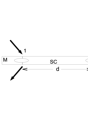
Figure 1: Non-local beam splitter and electron spin entangler. The MBS are shown as empty ellipses $1$ and $2$. One specific realization where MBS occur at boundaries between magnets (M) and superconductors (SC) deposited on quantum spin-Hall insulators is depicted, though our results hold more generally. Incoming and outgoing particles are shown by arrows, and may, in practice, be tunneled in/out by STM tips or electron pumps acting as leads.

II Nearly resonant electron (hole) scattering from Majorana edge states

We consider a one dimensional device supporting two weakly coupled MBS at its ends as shown in Fig.1. The MBS are labeled as $1$ and $2$ and schematically shown as empty ellipses in the figure. As the separation between the MBS increases their energy $E_{M}$ decreases exponentially Sodano . For the sake of clarity, we will first show how this device produces Hanbury Brown-Twiss like interference effects between spatially separated Dirac fermions in the spinless models investigated in Kitaev2 ; Sodano ; later, we show how all the results are valid for more realistic spinfull physical settings Fu-Kane1 ; Das-Sarma2 ; Refael1 . The Hamiltonian describing the weak coupling between the MBS $\gamma_{1}$ and $\gamma_{2}$ is given by

$$H_{M}=iE_{M}\gamma_{1}\gamma_{2},$$ (1)

where $\gamma_{j}$ are Majorana operators defined by $\gamma_{j}=\gamma_{j}^{\dagger}$ and satisfying $\gamma_{j}\gamma_{k}+\gamma_{k}\gamma_{j}=2\delta_{kj}$ (in our definition, the $\gamma_{j}=c_{j}+c_{j}^{\dagger}$ in terms of Dirac fermionic operators $c_{j}$).

Leads, also labeled as $1$ and $2$, are connected to the device as shown in Fig.1, allowing for the scattering of Dirac fermions (electrons or holes) from each of the MBS; we further assume that lead $1$ is coupled only to bound state $1$ while lead $2$ only to bound state $2$. The Hamiltonian describing the leads needs not to be specified at this stage since- for the evaluation of the S-matrix- the leads my be effectively removed by introducing complex embedding potentials datta . Using the approach developed in datta ; ghur one may then write the unitary scattering matrix $S$ in a form which is formally independent on the model used to describe the leads; for the scattering of fermions from the MBS located at the the ends of the quantum wire shown in Fig.1 the $S$ matrix has been computed in Beenakker as

$$S(E)=1+2\pi iW^{\dagger}(H_{M}-E-i\pi WW^{\dagger})^{-1}W$$ (2)

where $W$ is a rectangular matrix

$$\left(\begin{array}[]{cccc}~{}w_{1}&0&w_{1}^{\star}&0\\ ~{}0&~{}w_{2}&~{}0&w_{2}^{\star}\end{array}\right)$$

in the basis $\{|e_{1}\rangle,|e_{2}\rangle,|h_{1}\rangle,|h_{2}\rangle\}$, with $|e_{j}\rangle$ and $|h_{j}\rangle$ representing an electron and a hole in the lead $j$. $W$ describes the coupling of the scatterer ($H_{M}$) to the leads and $E$ is the energy of the incident electrons/holes. The entries $w_{j}$ of the $W$ matrix are related to the couplings to the leads $\Gamma_{j}=2\pi w_{j}^{2}$ Beenakker .

For our purposes, it is convenient to assume that $E>>\Gamma_{j}$, as well as $E\approx E_{M}$ (i.e., the energies of the incoming Dirac fermions are tuned to be nearly resonant with the Majorana coupling energy). Under these circumstances, the $S$ matrix simplifies to

$$S=\frac{1}{2}\left(\begin{array}[]{cccc}~{}1&-i&-1&-i\\ ~{}i&~{}1&~{}i&-1\\ -1&-i&~{}1&-i\\ ~{}i&-1&~{}i&~{}1\end{array}\right)$$ (3)

where the basis is, again, $\{|e_{1}\rangle,|e_{2}\rangle,|h_{1}\rangle,|h_{2}\rangle\}$. Note that this regime is different from the one considered by Akhmerov et. al. Beenakker , where only the terms corresponding to crossed Andreev reflection (i.e $\langle h_{2}|S|e_{1}\rangle$ and $\langle h_{1}|S|e_{2}\rangle$) are maximized. Here, we work in a regime where all the entries of $S$ have the same magnitude. It is the implications of this scattering matrix $S$ of Eq.(3) that we work out in this paper. It is this $S$ that enables both the non-local Hanbury-Brown Twiss interferometry in isospin space and the non-local entanglement generation.

Let us first illustrate the action of the above $S$ matrix by describing what happens to electrons tunneling in from one end of the one dimensional device. If, at time $t$, a single electron tunnels into the Majorana mode located at site 1, i.e., the incoming state is $c^{\dagger}_{1}|0\rangle$, it transforms, under $S$, to

$$c^{\dagger}_{1}|0\rangle\xrightarrow{\text{MBS}}\frac{1}{2}(c^{\dagger}_{1}+ic^{\dagger}_{2}-d^{\dagger}_{1}+id^{\dagger}_{2})|0\rangle,$$ (4)

where $c^{\dagger}_{j}$ ($d_{j}^{\dagger}$) creates an electron (hole) at site $j$. In Eq.(4), we have used MBS above the arrow to indicate that Majorana bound states are responsible for the process. Since the transformation (4) is equivalent to a four port beam splitter, with MBS inducing the beam splitting process, one can equally well take MBS to stand for “Majorana Beam-Splitter”. Eq.(4) implies that an incoming electron has $\frac{1}{4}$th probability of coming out of each site as an electron or a hole. If another electron scatters at a different time $t^{\prime}$ on the Majorana mode located at position 2, it will also scatter with exactly the same probabilities for the four possible outcomes. The joint probability for two incoming electrons to exit as two electrons or two holes (whichever the output port) would thus be $\frac{1}{2}$.

III Hanbury-Brown effect in pseudo-spin space

We will now show that when $t=t^{\prime}$, i.e., simultaneous scattering, two particle interference can take place so that the probability of two electrons or two holes exiting is completely suppressed. By $t=t^{\prime}$ we mean that the wavepackets of the two incoming electrons (holes) are large enough so that their time of arrival cannot be distinguished when one observes them after the scattering.

When two electrons scatter simultaneously, one at site 1 and the other at site 2, one has

$$c^{\dagger}_{1}c^{\dagger}_{2}|0\rangle \xrightarrow{MBS} \frac{1}{2}(c^{\dagger}_{1}+ic^{\dagger}_{2}-d^{\dagger}_{1}$$ (5)

$$+id^{\dagger}_{2})~{}~{}\frac{1}{2}(-ic^{\dagger}_{1}+c^{\dagger}_{2}-id^{\dagger}_{1}-d^{\dagger}_{2})|0\rangle$$

$$= \frac{1}{2}(ic^{\dagger}_{1}d^{\dagger}_{1}-c^{\dagger}_{1}d^{\dagger}_{2}+c^{\dagger}_{2}d^{\dagger}_{1}+ic^{\dagger}_{2}d^{\dagger}_{2})|0\rangle.$$

In the last step of Eq.(5), we have used $d^{\dagger}_{j}(E)=c_{j}(-E)$ (which effectively embodies the indistinguishability between an electron and a hole), where $E$ is energy. From Eq.(5) one sees that the probability for two outgoing electrons (holes) after the scattering is zero. Exactly the same holds when two holes scatter simultaneously at leads 1 and 2. This is an interference effect in the same sense as the anti-bunching of fermions at a normal two port beam splitter, where fermions cannot exit through the same port. Instead of being in the spatial channels, here the anti-bunching is in the internal pseudospin space which has particle and hole as its two states. The unitary conversion of an electron to a hole, is, per se, not surprising in view of Refs.Fu-Kane2 .

Of course, in a practical realization, the condition $E\sim E_{M}$ required for obtaining the scattering matrix $S$ of Eq.(3) may not be exactly met. To see the effect of an energy mismatch, we denote by $\delta E$ the amount by which $E$ deviates (either positively or negatively) from $E_{M}$; this deviation is, however, assumed to be much lower than $E_{M}$ itself (i.e., $\delta E<<E_{M}$). Without assuming $\delta E<<E_{M}$, one may end up in qualitatively different regimes: e.g., for $\delta E$ comparable to $-E_{M}$, one reaches the regime of Ref.Beenakker of only crossed transmission. For $\delta E<<E_{M}$, the scattering matrix as a function of $\delta E$ is given by

$$S_{\delta E}=\frac{i\Gamma}{\delta E+i\Gamma}S+\frac{\delta E}{\delta E+i\Gamma}I$$ (6)

where $\Gamma=\Gamma_{1}\sim\Gamma_{2}$ and $I$ is the $4\times 4$ identity matrix. In deriving Eq.(6), one ignores the second and higher powers of both $\delta E/E_{M}$ and $\Gamma/E_{M}$ as $E_{M}>>\Delta E,\Gamma$. It is easy to check that, despite the above approximation, $S_{\delta E}$ is unitary; furthermore, Eq.(6) holds for any value of the ratio $\delta E/\Gamma$ as long as $E_{M}>>\Delta E,\Gamma$. Using $S_{\delta E}$, one readily obtains that the probability of observing an electron-electron output state becomes finite and equal to $\frac{(\delta E)^{2}}{(\delta E)^{2}+\Gamma^{2}}$, which, of course, vanishes when $E\sim E_{M}$.

Before ending this section, as a brief aside, we point out that, when one electron and one hole scatter at sites $1$ and $2$ respectively, for $\delta E<<\Gamma$, the incoming state $c^{\dagger}_{1}d^{\dagger}_{2}|0\rangle$ evolves to $\frac{1}{2}(-c^{\dagger}_{1}c^{\dagger}_{2}-ic^{\dagger}_{1}d^{\dagger}_{1}+ic^{\dagger}_{2}d^{\dagger}_{2}-d^{\dagger}_{1}d^{\dagger}_{2})|0\rangle$, implying the interferometric vanishing of the probability of one outgoing electron and one outgoing hole in separate leads. We will not delve further into this case, but next proceed to discuss the signatures of the Hanbury-Brown interferometry in the case of two incident electrons.

IV Spectral density of current fluctuations: a signature of fermion antibunching in pseudospin space

In the previous section we have described the scattering as a process where one sends particles one by one through the leads at specific times. However, in practice, rather than controlling times, one could control the energies $\epsilon_{1}$ and $\epsilon_{2}$ of the particles in their respective leads, so as to make them behave indistinguishably when $\epsilon_{1}\sim\epsilon_{2}$. Then, the standard way to observe the predicted fermion anti-bunching is through a measure of the correlations between the currents in leads $1$ and $2$. The current in lead $j$ may be written as buttiker ; loss-burkard

$$I_{j}(t)=\frac{e}{h\nu}\sum_{\epsilon,\epsilon^{{}^{\prime}}}e^{i(\epsilon-\epsilon^{{}^{\prime}})t}\{a_{j}^{\dagger}(\epsilon)a_{j}(\epsilon^{{}^{\prime}})-b_{j}^{\dagger}(\epsilon)b_{j}(\epsilon^{{}^{\prime}})\}$$ (7)

where $a_{j}$ and $b_{j}$ denote the incoming and outgoing particles and $\epsilon$ and $\epsilon^{{}^{\prime}}$ are the energies of the particles and $\nu$ is the density of states of the incoming electrons. The spectral density of the current fluctuations $\delta I_{j}=I_{j}-\langle I_{j}\rangle$ between the leads at zero frequency is loss-burkard

$$P_{ij}=\text{lim}_{~{}T\rightarrow\infty}\frac{h\nu}{T}\int_{0}^{T}dt~{}\text{Re}\langle\delta I_{1}(t)\delta I_{2}(0)\rangle.$$ (8)

Using $S_{\delta E}$ of Eq.(6) and considering an incoming two electron state $c^{\dagger}_{1}(\epsilon_{1})c^{\dagger}_{2}(\epsilon_{2})|0\rangle$, where $c^{\dagger}_{j}(\epsilon_{j})$ denotes an electron of energy $\epsilon_{j}$ in lead $j$, one finds

$$P_{ij}=\frac{e^{2}}{h\nu}\frac{\Gamma^{2}}{\{(\delta E)^{2}+\Gamma^{2}\}^{2}}\{(\delta E)^{2}-\Gamma^{2}\}\delta_{\epsilon_{1},\epsilon_{2}},$$ (9)

where $\delta_{\epsilon_{1},\epsilon_{2}}$ is the Kronecker delta function. Note that, when the incident electrons are distinguishable i.e., $\epsilon_{1}\neq\epsilon_{2}$, then, as expected, $P_{ij}=0$ since for an electron exiting one lead there could equally well be an electron or a hole exiting the other lead. When, instead, $\epsilon_{1}=\epsilon_{2}$ (i.e., the particles are indistinguishable), then for $|\delta E|<|\Gamma|$, the domination of the electron-hole final state (as in Eq.(5)) makes $P_{ij}<0$, which allows to the detect the predicted “anti-bunching” in pseudospin space. For $|\delta E|>|\Gamma|$ a process of amplitude $\Gamma\delta E$ in which only one of the electrons scatter, while the other remains in its lead, dominates; Fermi statistics now makes the electrons anti-bunch spatially (the more conventional antibunching yamamoto ; loss-burkard ), contributing to a positive $P_{ij}$. As in Ref.Beenakker , our results are not inconsistent with those of Bolech and Demler Bolech-Demler , since their results apply when the energy of the incoming electrons is much higher than $E_{M}$.

V Scattering Matrix in the spinfull case

So far our analysis has been confined to the spinless model investigated in Sodano ; Beenakker , while for the promising implementations Fu-Kane1 ; Das-Sarma2 ; Refael2 ; Refael1 , the Majorana modes should involve superpositions of operators of different spins. For example, for a realization in a ferromagnet-s-wave superconductor-ferromagnet structure on a quantum spin-Hall edge Refael2 , one has

$$\gamma_{1}=\frac{1}{\sqrt{2}}(c_{1,\uparrow}-ic_{1,\downarrow}+ic_{1,\downarrow}^{\dagger}+c_{1,\downarrow}^{\dagger})$$

$$\gamma_{2}=\frac{1}{\sqrt{2}}(c_{2,\uparrow}+ic_{2,\downarrow}-ic_{2,\downarrow}^{\dagger}+c_{2,\downarrow}^{\dagger}),$$ (10)

where $c_{j,\sigma}$ creates an electron with spin $\sigma$ in lead $j$. Defining the spin states $|\pm y\rangle=\frac{1}{\sqrt{2}}(|\uparrow\rangle\pm i|\downarrow\rangle)$, and using the basis $\{|e_{1,+y}\rangle,|e_{2,-y}\rangle,|h_{1,+y}\rangle,|h_{2,-y}\rangle,|e_{1,-y}\rangle,|e_{2,+y}\rangle,|h_{1,-y}\rangle,$ $|h_{2,+y}\rangle\}$, the scattering matrix is found to be

$$S_{\text{spinfull}}=\left(\begin{array}[]{cc}~{}I&~{}{\bf 0}\\ ~{}{\bf 0}&~{}S\end{array}\right),$$ (11)

where in (11), $I$ and ${\bf 0}$ are the $4\times 4$ Identity and null matrices, while $S$ is the scattering matrix given by Eq.(3).

When one uses $S_{\text{spinfull}}$ to study the scattering of the incident state $c_{1,-y}^{\dagger}c_{2,+y}^{\dagger}|0\rangle$, one only needs the lower-right $4\times 4$ block of $S_{\text{spinfull}}$. Thus, precisely the same electron-hole output state as in Eq.(5) is obtained, apart from the fact that, now, the spin indices $-y$ and $+y$ are pinned to the sites $1$ and $2$ respectively. Thus, by choosing the spin polarizations of the incoming electrons pertinently, one can observe all the effects described till now. This should be possible in a variety of systems as Majorana modes of the form given by Eq.(10) are quite generic, e.g., also realizable in semiconductor-superconductor-magnet structures Refael1 .

VI Entanglement of distant electron spins

We now propose a protocol for the generation of entanglement between spins of well separated particles incoming at site 1 and at site 2. For this purpose, we choose the realization of Majorana fermions given by Eq.(10) and make two electrons with parallel spins in the $\uparrow$ direction come in simultaneously i.e., choose the initial state $c_{1,\uparrow}^{\dagger}c_{2,\uparrow}^{\dagger}|0\rangle$. Then, using $S_{\text{spinfull}}$, one gets

$$c_{1,\uparrow}^{\dagger}c_{2,\uparrow}^{\dagger}|0\rangle \xrightarrow{MBS} \frac{1}{4}(c_{1,\uparrow}^{\dagger}c_{2,\uparrow}^{\dagger}-c_{1,\downarrow}^{\dagger}c_{2,\downarrow}^{\dagger}+2c_{1,\uparrow}^{\dagger}c_{2,\downarrow}^{\dagger}$$ (12)

$$+ ...)|0\rangle,$$

where $...$ denotes terms such as $c_{1,\sigma}^{\dagger}c_{1,\sigma^{{}^{\prime}}}^{\dagger},c_{2,\sigma}^{\dagger}c_{2,\sigma^{{}^{\prime}}}^{\dagger},c_{j,\sigma}^{\dagger}d_{k,\sigma^{{}^{\prime}}}^{\dagger}$ and $d_{j,\sigma}^{\dagger}d_{k,\sigma^{{}^{\prime}}}^{\dagger}$, which are not relevant to our discussion. Eq.(12) implies that, when two outgoing electrons are obtained in leads $1$ and $2$ separately, their state is $|\xi\rangle_{12}=\frac{1}{\sqrt{6}}(|\uparrow\rangle_{1}|\uparrow\rangle_{2}-|\downarrow\rangle_{1}|\downarrow\rangle_{2}+2|\uparrow\rangle_{1}|\downarrow\rangle_{2})$ where, as it is usually done Bose-Home ; loss-burkard , one uses the lead label to label the electron. $|\xi\rangle_{12}$ is an entangled state of the spins of electrons $1$ and $2$, with the amount of entanglement (as quantified by the von Neumann entropy of one of the particles entconc ) being $0.19$ ebits. Though the entanglement is not very high, $|\xi\rangle_{12}$ is a pure state, and hence of value in quantum information, as its entanglement can be concentrated without loss by local means entconc . Moreover, the probability of obtaining two outgoing electrons in separate leads (i.e., $|\xi\rangle_{12}$) is rather high, namely $3/8$. At the expense of decreasing this probability, one may improve the degree of entanglement of the generated state by tuning the polarizations of the incoming electrons. For instance, if the incoming state is $(\frac{1}{\sqrt{10}}c_{1,+y}^{\dagger}+\frac{3}{\sqrt{10}}c_{1,-y}^{\dagger})(\frac{3}{\sqrt{10}}c_{2,+y}^{\dagger}+\frac{1}{\sqrt{10}}c_{2,-y}^{\dagger})|0\rangle$, one obtains an output state of entanglement $0.75$ ebits, while the probability of the generation this state becomes $0.055$. The spin entanglement of the outgoing electrons could be measured by passing them through separate spin filters as in Ref. martin .

Unlike the entanglement generation scheme of Ref. Bose-Home , here particles polarized parallel to each other suffice to generate entanglement. Importantly, in our protocol, particles at a distance from each other can be made entangled; this may avoid the decoherence arising necessarily from the transport needed to separate the particles after a local entangling mechanism. In addition, the distance between the entangled particles can be enhanced by putting $n$ copies of our setup in series with leads connecting the end of one copy to the beginning of another. The probability of obtaining the state $|\xi\rangle_{12}$ in the leftmost and rightmost leads will then be $(3/8)^{n}$.

One might think that in analogy with Ref.loss-burkard , perhaps it is possible also to detect entanglement between distant electronic spins by injecting to the opposite ends of our one dimensional device. As a maximally entangled state of two spins can be written in any basis, let us consider the $|\pm y\rangle$ basis for spins. In this basis, two of the maximally entangled states can be written as $|\psi^{\pm}\rangle_{12}=(c^{\dagger}_{1,+y}c^{\dagger}_{2,-y}\pm c^{\dagger}_{1,-y}c^{\dagger}_{2,+y})|0\rangle$. The detection of entanglement at a normal 50-50 beam splitter relies crucially on both the incoming states $c^{\dagger}_{1,+y}c^{\dagger}_{2,-y}|0\rangle$ and $c^{\dagger}_{1,-y}c^{\dagger}_{2,+y}|0\rangle$ evolving at the beam-splitter and interference (i.e., cancellation/addition) between the terms resulting from the evolution each of the above two states. Only as a result of these cancellations/additions does the bunching/anti-bunching effects evidencing entanglement arise. However, here the term $c^{\dagger}_{1,+y}c^{\dagger}_{2,-y}|0\rangle$ does not even evolve under the action of $S_{\text{spinfull}}$ so that interferences are impossible. Thus though our device can generate spin entanglement it cannot detect spin entanglement.

VII A few condensed matter settings

One simple setting where the non-local two particle interferometry and the entanglement generation between distant electrons from MBS may be observed can be engineered with magnet-superconductor-magnet junctions deposited on the edge of a 2D quantum spin Hall insulator Beenakker ; Refael2 . Just as in Ref.Beenakker , one can observe these effects when the Majorana modes are separated by a distance $d$ of several micrometers at temperatures of the order of 10 mK. For this setting, the explicit form of the Majorana operators is exactly the same as in Eq.(10) Refael2 . Interestingly, strong spin-orbit coupled quantum wires in proximity with ferromagnets and superconductors also support the realization of MBS Das-Sarma2 ; Refael1 given in Eq.(10) Refael1 . As in previous proposals Bolech-Demler ; Das-Sarma2 ; Refael2 , also in these settings, two STM tips could act as the leads $1$ and $2$ to observe the non-local two particle Hanbury Brown-Twiss interferometry. For the entanglement generation, instead, it will be more useful to have synchronized electron pumps Pepper feeding in the incoming electrons. In addition, the filtering of the desired state $|\xi\rangle_{12}$ can be achieved by pumps capturing exactly one outgoing electron from each Majorana bound state.

VIII Conclusions

In this paper, we showed that a one dimensional device with two Majorana bound states at its ends yields a Hanbury-Brown Twiss effect in the internal electron-hole pseudospin space which may be detected in realistic condensed matter settings through current-current correlations. This is a departure from all the known multi-particle interference effects which have manifested themselves in spatial bunching and antibunching or spin-spin correlations. Fundamentally, it can be regarded as a manifestation of the quantum indistinguishability between electronic annihilation and hole creation evidencing the presence of Majorana bound states. The same settings may also be used to engineer a non-local entangler of distant electronic spins, which may enable circumventing the decoherence arising from the transport needed to separate entangled particles.

Acknowledgements: We thank C. Chamon, R. Egger, R. Jackiw, M. Pepper, S. Y. Pi, G. W. Semenoff and S. Tewari for fruitful discussions. SB (PS) thanks the University of Perugia (University College London) for hospitality and partial support. SB thanks the EPSRC, UK, the Royal Society and the Wolfson Foundation.

References

- (1) C. K. Hong, Z. Y. Ou, and L. Mandel, Phys. Rev. Lett. 59, 2044 (1987).
- (2) R. C. Liu et. al., Nature 391, 263-265 (1998).
- (3) T. Jeltes et. al., Nature 445, 402 (2007).
- (4) Y. H. Shih and C. O. Alley, Phys. Rev. Lett. 61, 2921 2924 (1988).
- (5) S. Bose and D. Home, Phys. Rev. Lett. 88, 050401 (2002).
- (6) L. Fu and C. L. Kane, Phys. Rev. Lett. 102, 216403 (2009); A. R. Akhmerov, J. Nilsson and C. W. J. Beenakker, Phys. Rev. Lett. 102, 216404 (2009)
- (7) G. W. Semenoff and P. Sodano, J. Phys. B: At. Mol. Opt. Phys. 40, 1479 (2007).
- (8) J. Nilsson, A.R. Akhmerov, and C.W.J. Beenakker, Phys. Rev. Lett. 101, 120403 (2008).
- (9) L. Fu, Phys. Rev. Lett. 104, 056402 (2010).
- (10) A. Yu. Kitaev, Phys.-Usp. 44, 131 (2001).
- (11) S. Tewari et. al, Phys. Rev. Lett. 98, 010506 (2007).
- (12) L. Fu and C. L. Kane, Phys. Rev. Lett. 100, 0964407 (2008).
- (13) V. Shivamoggi, G. Refael, and J. E. Moore, Phys. Rev. B 82, 041405 (2010).
- (14) J. D. Sau et. al, arXiv:1006.2829v2 (2010); J. D. Sau et. al, Phys. Rev. Lett. 104, 040502 (2010).
- (15) Y. Oreg, G. Refael, F. von Oppen, arXiv:1003.1145v2 (2010).
- (16) C. Chamon et. al., Phys. Rev. B 81, 224515 (2010).
- (17) A. Yu. Kitaev Ann. Phys. (N.Y.) 303, 1 (2003); C. Nayak et. al, Rev. Mod. Phys. 80, 1083 (2008).
- (18) S. Datta Electronic Transport in Mesoscopic Systems, (Cambridge University Press, 1995),pp. 145-157; D.S. Fisher and P. A. Lee, Phys. Rev. B 23, 6851 (1981).
- (19) T. Ghur, A. Müller-Groeling, H. Weidenmuller, Phys. Rep. 299, 189-425 (1998).
- (20) M. Büttiker, Phys. Rev. Lett. 65, 2901 (1990).
- (21) G. Burkard, D. Loss, E. V. Sukhorukov, Phys. Rev. B 61, R16303 (2000).
- (22) C. J. Bolech and E. Demler, Phys. Rev. Lett. 98, 237002 (2007).
- (23) O. Sauret, T. Martin, D. Feinberg, Phys. Rev. B 72, 024544 (2005).
- (24) C. H. Bennett et. al, Phys. Rev. A 53, 2046 (1996).
- (25) M.D. Blumenthal al., Nat. Phys. 3 343 (2007); S. J. Wright et. al., Phys. Rev. B 80, 113303 (2009).