The Larson-Tinsley Effect in the UV: Interacting vs. ‘Normal’ Spiral Galaxies

Abstract

We compare the UV-optical colors of a well-defined set of optically-selected pre-merger interacting galaxy pairs with those of normal spirals. The shorter wavelength colors show a larger dispersion for the interacting galaxies than for the spirals. This result can best be explained by higher star formation rates on average in the interacting galaxies, combined with higher extinctions on average. This is consistent with earlier studies, that found that the star formation in interacting galaxies tends to be more centrally concentrated than in normal spirals, perhaps due to gas being driven into the center by the interaction. As noted in earlier studies, there is a large variation from galaxy to galaxy in the implied star formation rates of the interacting galaxies, with some galaxies having enhanced rates but others being fairly quiescent.

1 Introduction

In a ground-breaking study, Larson & Tinsley (1978) found that the broadband optical UBV colors of interacting galaxies have a larger scatter than normal galaxies. Using population synthesis modeling, they concluded that this scatter was caused by bursts of star formation triggered by the interaction, superimposed on an older stellar population. Since then, a number of studies at other wavelengths have confirmed this basic result. For example, statistical studies of the H$\alpha$ equivalent widths, H$\alpha$ luminosity per unit area, far-infrared to blue luminosity ratios, and mid-infrared colors of interacting galaxies imply that their mass-normalized star formation rates are enhanced by a factor of two on average compared to normal spirals (Kennicutt et al., 1987; Bushouse, 1987; Bushouse, Lamb, & Werner, 1988; Barton et al., 2000; Barton Gillespie, Geller, & Kenyon, 2003; Smith et al., 2007). Statistical analyses of the optical spectra of large samples of galaxies also support the idea that close interactions can enhance star formation (Lambas et al., 2003; Li et al., 2008).

With the advent of the Galaxy Evolution Explorer (GALEX) ultraviolet telescope (Martin et al., 2005), a new window on star formation in galaxies became available. Not only is the UV a sensitive tracer of star formation, but adding the UV to optical datasets helps break the age$-$extinction degeneracy in population synthesis modeling (e.g., Smith et al., 2008). In addition, since the UV traces somewhat older and lower mass stars ($\leq$400 Myrs; O to early-B stars) than H$\alpha$ ($\leq$10 Myrs; early- to mid-O stars), it provides a measure of star formation over a longer timescale than H$\alpha$ studies. Furthermore, since UV-bright stars are more abundant than the stars traced by H$\alpha$ studies, UV photometry is a better tool to use to study star formation rates, efficiencies, and thresholds in regions with low gas surface density (Boissier et al., 2007). For example, GALEX observations have revealed star formation in the outermost reaches of spiral galaxies, unseen by H$\alpha$ studies (Thilker et al., 2005a, b; Gil de Paz et al., 2005). In interacting galaxies, tidal features are sometimes quite prominent in the UV compared to the optical (Neff et al., 2005; Smith et al., 2010).

At the present time, the mechanisms by which interactions trigger star formation are not well-understood. These include gas compression, shocks, cloud collisions, threshold effects, Schmidt-type star formation laws, stochastic processes, and mass transfer in and between galaxies (e.g., Keel, 2010). The importance of each of these processes in star formation initiation in interacting galaxies is not yet well-determined. Detailed multi-wavelength analyses of individual star forming regions within galaxies, including UV data, in conjunction with numerical modeling of the interaction, provides a good way to determine which processes are more important in an individual galaxy (e.g., Hancock et al., 2007, 2009; Smith et al., 2008, 2010; Peterson et al., 2009). To get an indication of the overall importance of each mechanism to star formation triggering in interacting galaxies, statistical studies of global properties are also useful.

At present little statistical information is available about how the global UV$-$optical colors and the UV luminosities of interacting galaxies compare to normal spirals. In general, interpreting the UV-optical colors of galaxies in terms of star formation enhancements is more difficult than using H$\alpha$, mid-, and far-infrared measurements, because of an increased sensitivity to extinction and the fact that the UV is sensitive to both young and intermediate-aged stars. Furthermore, the global UV/optical colors of galaxies are strongly affected by the distribution of dust relative to the stars, and therefore by the morphological type of the galaxy. To address these issues, we have conducted a study that involves a large multi-wavelength database for a well-defined sample of nearby pre-merger interacting pairs, and a matching dataset for a comparison sample of ‘normal’ spirals.

2 The Interacting Galaxy Sample and Database

Over the last several years, we have been conducting a large observational study of a sample of more than three dozen pre-merger interacting galaxy pairs (the ‘Spirals, Bridges, and Tails’ (SB&T) sample; Smith et al., 2007, 2010). These galaxies were selected from the Arp (1966) Atlas of Peculiar Galaxies to be relatively isolated binary systems with strong tidal distortions; we eliminated merger remnants, close triples, and multiple systems, unless the additional galaxies were relatively low mass. Our systems all have radial velocities $<$10,350 km s^-1 and angular sizes $\geq$3^′. The interacting pair NGC 4567 was added to the sample, since it fits these criteria but is not in the Arp Atlas. Since these galaxies are relatively simple pre-merger systems, they are more amendable to the detailed matching of simulations to observations (e.g., Struck & Smith, 2003) than merger remnants. Thus this sample provides a good testbed for investigating interaction-induced star formation.

The dataset for the SB&T sample includes mid-infrared imaging with NASA’s Spitzer space telescope (Smith et al., 2005, 2007; Hancock et al., 2007) as well as ultraviolet imaging with GALEX (Hancock et al., 2007; Smith et al., 2010). In addition, broadband ugriz optical images are available for most of the sample galaxies from the Sloan Digitized Sky Survey (SDSS; Abazajian et al., 2003). We have already produced an Atlas of the Spitzer infrared images (Smith et al., 2007) and a second Atlas of the GALEX and SDSS images (Smith et al., 2010). In an earlier study (Smith et al., 2007), we compared the Spitzer broadband mid-infrared colors of this sample with those of a control sample of ‘normal’ spirals selected from the Kennicutt et al. (2003) SINGS sample by eliminating strongly interacting galaxies. Multi-wavelength studies of individual galaxies in the sample have been presented by Hancock et al. (2007, 2009), Smith et al. (2005, 2008), and Peterson et al. (2009).

3 A Large ‘Control’ Sample of Spirals

The next step is to test whether the UV emission from our sample galaxies is also enhanced by the interactions, and if there is a statistically-significant difference in the UV-optical colors of our galaxies compared to spirals. Unfortunately, however, only a subset of the ‘control’ sample of ‘normal’ spirals we used in our earlier Spitzer study (Smith et al., 2007) has reliable optical magnitudes available (Mñoz-Mateos et al., 2009), and the final sample size is too small for a valid comparison. No other appropriate control sample with both UV and optical data is currently available in the literature.

To address this lack, we have constructed a new control sample. To ensure the availability of high quality UV data ($\geq$ 1 orbit observing time with GALEX), we started with the 1034 galaxies in the ‘GALEX Ultraviolet Atlas of Nearby Galaxies’ (Gil de Paz et al., 2007). This contains most of the large angular size galaxies in the local Universe that have been observed by GALEX to date. We selected the subset of these galaxies classified as Sa $-$ Sd spirals in the Gil de Paz et al. (2007) tabulation, and searched the NASA Extragalactic Database (NED) for companions. We eliminated galaxies with companions that have velocity differences $<$ 1000 km s^-1, separation on the sky $<$ 10 $\times$ (diameter of target + diameter of companion), and optical magnitude(companion) $<$ 1.5 + magnitude(target galaxy). We then limited the resultant sample to galaxies with distances between 6.2 $-$ 143 Mpc, the range of distances in the SB&T sample. We then omitted galaxies with angular sizes larger than the SDSS field of view of $\sim$8^′ and galaxies split between two SDSS or GALEX images. We inspected the images for previously-unidentified morphological peculiarities and companions, as well as artifacts in the images. We eliminated such galaxies, leaving a final sample of 121 galaxies. Of these galaxies, only five are listed as possible Seyferts in NED, compared to nine out of the 84 main galaxian disks in the 42 SB&T pairs.

As noted above, we selected our spiral sample to have the same range of distances as the SB&T sample. This is shown in Figure 1, where we provide histograms of the distances to the galaxies in the two samples. On average, the spirals are slightly more distant, with a median distance of 68 Mpc, vs. 37 Mpc for the SB&T galaxies. A K-S test give a probability that the two sets of distances are drawn from the same parent population of 3.3%, thus the difference between these two samples is marginally significant.

This sample and the SB&T sample both contain mostly high latitude galaxies. The distributions of Galactic latitudes b for the two samples are shown in Figure 2. Almost all the galaxies have $|$b$|$ $>$ 25^∘, with the median $|$b$|$ being 54^∘ for the SB&T sample and 48^∘ for the comparison spirals. A K-S test gives a probability of 1.1% that the two distributions come from the same parent sample, thus there is a significant difference between the two samples. However, this is unlikely to have a large effect on our results, since at these latitudes the corrections for Galactic extinction are small.

4 The Large-Scale Environment

In addition to the presence of nearby neighbors, another factor that affects galaxian star formation rates is the large scale environment, i.e., whether the galaxy is in a group, cluster, or the field (e.g., Gómez et al., 2003). Therefore, in constructing a comparison sample, it is important to also compare the large scale environment of the galaxies (e.g., Sol Alonso et al., 2006; Barton et al., 2007). To this end, for our sample ‘normal’ galaxies, we have used NED to determine the number of neighboring galaxies. We used a search radius of 2 Mpc, a velocity difference of $\leq$ 1000 km s^-1, and an absolute magnitude limit for the neighbor of M_V = $-$18.5 (approximately equal to that of the Large Magellanic Cloud). This search was constrained by the maximum search radius in NED of 300 arcminutes, thus is deficient for very nearby galaxies ($<$23 Mpc), however, this only affects a small number of galaxies in the two samples (see Figure 1).

Histograms of the number of neighbors that fit these criteria are given in Figure 3 for the two samples of galaxies. This figure shows four outliers in the SB&T sample, in very dense environments. In order from right to left, these are Arp 105 (in the Abell 1185 cluster), Arp 120 (in the Virgo cluster), Arp 65 (in the WBL 009 cluster), and NGC 4567 (in Virgo). Other than these outliers, the two distributions are similar. A KS test gives a 44% chance that the two distributions arise from the same parent population, thus environmental differences between the two samples are statistically insignificant.

5 Morphological Types

To better interpret any possible differences in UV-optical colors between these two samples, we first compare the morphological types of the individual galaxies in the samples. To this end, we used NED to extract morphological types for the individual galaxies in the SB&T pairs, as well as for the spiral sample. These types are plotted as histograms in the top and middle panels of Figure 4. For these histograms, we ignored any notes in NED on morphological peculiarities (i.e., Sab Pec), and just used the basic Hubble type (i.e., Sab). The fact that many of these galaxies are peculiar, combined with the fact that the types in NED are inhomogeneous and subjective, means that there are significant uncertainties in the types plotted in Figure 4. However, to first order these histograms suggest that the two sets of galaxies are different morphologically, in addition to the presence of tidal features in the SB&T galaxies. For example, the SB&T sample contains quite a few galaxies classified as S0 and Im/Irr/Sm, as well as a few ellipticals. In contrast, the spiral sample was intentionally selected to avoid these types. Furthermore, the distribution of types for the SB&T galaxies peaks at Sb, while that for the spiral sample peaks at Sc/Scd. This suggests a possible difference in the bulge/disk ratios of the two samples.

The two samples appear to have similar fractions of barred spirals. About 30% of the spirals in the interacting sample are classified as SB in NED, compared to 33% in the comparison spiral sample. For the interacting sample, 14% of the spirals are listed as SAB in NED, compared to 19% of the comparison sample galaxies.

Since a strong interaction can change the appearance of a galaxy, the morphological types in NED do not necessarily reflect the original pre-interaction structures of the galaxies. Unfortunately, after the fact it is often difficult to tell original morphological types. It is unclear whether the skewing of the spiral subset of the SB&T sample to earlier Hubble types is due to a difference in progenitors caused by selection effects, to changes produced by the interaction itself, or to biases in the typing of the interacting galaxies.

To partially address the issue of morphological bias in the samples, in the following analyses we only include the SB&T galaxies with current morphological types in NED between S0/a and Sdm. Since the SB&T spirals are skewed to earlier Hubble types compared to the comparison spirals, in addition to comparing to the full comparison sample, we have repeated the analysis using Hubble-type-matched subsets of the comparison sample. These subsets were constructed by randomly selecting galaxies from the comparison sample to fit a fixed distribution of Hubble types which approximately matches the Hubble type distribution of the spirals in the SB&T sample. This fixed distribution is plotted in the third panel of Figure 4. These subsets have 61 galaxies each, thus contain approximately half of the original sample of comparison spirals. We randomly selected 100 such subsets, and ran the statistical tests with each subset, to investigate how much random chance affects the final statistics. These results are described below.

6 UV/Optical Magnitudes of Spiral Sample

For the galaxies in our spiral sample, we used the GALEX and SDSS images to extract total FUV, NUV, and ugriz magnitudes, using the same method as we used for the SB&T galaxies (Smith et al., 2007, 2010), including an additional term in the uncertainties to account for sky variations. Of the 121 spiral galaxies in our sample, 12 do not have FUV images available, thus FUV magnitudes are not available for these systems. We corrected the observed magnitudes for Galactic extinction in the same way as for the SB&T galaxies (Smith et al., 2010). The corrected magnitudes are given in Table 1.

7 Luminosity Comparisons

The next question is whether the luminosities and stellar masses of the two samples differ. In Figures 5 and 6 we plot the NUV and g luminosity distributions of the SB&T spiral sample and the full comparison sample, with the luminosities being calculated as $\nu$L_ν. For the SB&T sample, we plot the luminosities of the main disks separately from those of the tails and bridges. We also plot separately the luminosities of the candidate tidal dwarf galaxies (TDGs), as identified in Smith et al. (2010). Tidal dwarf galaxies are concentrations of young stars and gas in tidal features that may or may not evolve into independent dwarf galaxies.

The median fraction of the total galaxian luminosity in the tidal features plus that in the TDGs is $\sim$15% in the UV bands, and $\sim$10% in the optical. However, this fraction varies widely from galaxy to galaxy, ranging from $<$1% $-$ 65% in the UV bands, and $<$1% $-$ 40% in the optical. For comparison, for a different subset of Arp Atlas galaxies, Schombert, Wallin, & Struck-Marcell (1990) found an average of $\sim$25% of the total visible starlight was contained in tidal features. For the SB&T galaxies, in the Spitzer 3.6 $\mu$m $-$ 8 $\mu$m bands we found $\leq$10% of the light was coming from the tidal features on average (Smith et al., 2007).

The NUV luminosities for the disks of the comparison spirals are very slightly larger than for the SB&T spirals on average, with median luminosities of 10^43.0 erg sec^-1 and 10^42.8 erg sec^-1, respectively. If the light from the tidal features were combined with that of the SB&T disks, this would partially account for the difference. A K-S test give a probability that these two sets of luminosities came from the same sample of 33%, thus we cannot rule out the hypothesis that the two sets of data come from the same parent population. The median g luminosity for both the comparison spirals and the SB&T spirals are 10^43.5 erg sec^-1, with a K-S test giving a probability of the two parent populations being the same of 28%. Thus the g luminosities of the two samples are also not significantly different. The small difference in the distribution of distances for the two samples therefore does not produce a strong difference in luminosities. We conclude that there is likely not a large difference in the mass distribution for the two samples.

8 Color-Color Plots

The main result of the Larson & Tinsley (1978) study was that interacting galaxies show a larger scatter in the UBV color-color diagram than normal galaxies. To search for this effect in our dataset and to extend to other wavelengths, in Figures 7 $-$ 11 we provide various color-color plots for the full comparison sample of spirals (right panel), compared to the SB&T disks, excluding the E/S0/Sm/Im/Irr galaxies (left panel). Following Larson & Tinsley (1978), on these plots we include curves showing the running averages of the x-value for the comparison spirals (solid curves) and SB&T spirals (dotted curves) as a function of the y-value, calculated in bins of 0.1 magnitudes, except for NUV $-$ g, where we used 0.2 magnitude bins. These curves help guide the eye to see differences between the samples.

We calculated the rms deviation of each dataset relative to these mean lines. These values are given in Table 2. For the SB&T galaxies, we calculated the rms deviation relative to the mean curve for the SB&T sample itself (fourth column in Table 2), as well as the rms deviation relative to the mean curve for the full comparison spiral sample (fifth column). For the FUV $-$ NUV vs. g $-$ r, NUV $-$ g vs. g $-$ r, and u $-$ g vs. g $-$ r plots (Figures 7 $-$ 9), the rms deviations of the SB&T spirals are indeed larger than for the comparison spirals, especially when calculated compared to the mean line for the comparison spirals. In contrast, for the two longer wavelength color-color plots (Table 2 and Figures 10 and 11), there is little difference in the scatter, as expected for redder colors dominated mainly by the light from older stars.

We repeated this analysis with the Hubble-type-matched subsamples, and found similar results. In Table 2, we provide the mean rms deviations for our 100 randomly-selected subsets. On average, for the shorter wavelength colors, these subsets also show smaller scatter than the SB&T galaxies.

Inspection of these plots shows a few additional differences between the two samples. First, there is a subset of the SB&T spirals with significantly bluer NUV $-$ g colors for their g $-$ r values (Figure 8). Second, in Figure 9, the u $-$ g vs. g $-$ r plot, the datapoints for the interacting sample tend to lie to the right of the mean line for the comparison spirals (i.e., to redder u $-$ g values for a given g $-$ r). In g $-$ r vs. r $-$ i (Figure 10), a similar effect is seen: there is a slight tendency of the interacting sample towards redder g $-$ r values compared to r $-$ i. However, as noted above, the scatter relative to the mean spiral line for g $-$ r vs. r $-$ i is similar in both samples, so any systematic offset is small. In the other two color-color plots, FUV $-$ NUV vs. g $-$ r (Figure 7) and r $-$ i vs. i $-$ z (Figure 11), no systematic offset between the two samples is evident within the uncertainties. Inspection of similar color-color plots for the Hubble-type selected subsets shows similar trends.

9 Color-Morphology Relations

As noted earlier, there is a difference in the morphological types of the galaxies in the two spiral samples, with more Sb galaxies in the SB&T galaxies, and more Sc galaxies in the full comparison spiral set. To investigate further the relation between morphology and color, for both the SB&T galaxies and the full comparison sample, in Figures 12 $-$ 17 we compare the morphological types with FUV $-$ NUV, NUV $-$ g, u $-$ g, g $-$ r, r $-$ i, and i $-$ z, respectively. Clear trends are seen in these plots, in that earlier Hubble types are redder, as expected (e.g., de Vaucouleurs, 1977; Gil de Paz et al., 2007).

For each spiral Hubble type and each color for both sets of galaxies, we have calculated the mean color. These mean value curves are plotted on Figures 12 $-$ 17, with the solid curve being the mean values for the comparison sample, and the dotted curve the SB&T sample. In Table 3, we give the rms deviations of the datapoints relative to these curves. For the three shorter wavelength colors, these residuals are larger for the SB&T sample, reflecting either a larger range in star formation rates and/or extinctions for a given Hubble type for the interacting sample, and/or larger inaccuracies in Hubble typing.

At the shorter wavelengths, for some of the Hubble types there is a tendency for the mean colors of the interacting galaxies to be slightly redder than for the comparison spirals. However, this effect is slight. The main difference between the two samples is the somewhat larger scatter for the interacting galaxies.

We repeated this analysis for the Hubble-type-matched subsets of the comparison sample, and find similar results. The mean values for 100 type-match subsets are also given in Table 3.

10 Comparison with Previous Studies of Optical Colors

We find a significant difference in the optical colors of our spiral and interacting samples, with the interacting galaxies showing more dispersion in the colors. Our study thus confirms the basic results of Larson & Tinsley (1978), who saw greater scatter in the UBV optical colors for their sample of Arp galaxies than for galaxies from the Hubble Atlas of Galaxies (Sandage, 1961), using photometry from the Second Reference Catalogue of Bright Galaxies (de Vaucouleurs, de Vaucouleurs, & Corwin, 1976; RC2). However, there are some differences between that study and the current study. In their UBV color-color plot, Larson & Tinsley (1978) saw more scatter to the blue in U $-$ B for a given B $-$ V for the interacting galaxies compared to their control sample. In contrast, in our u $-$ g vs. g $-$ r plot, our interacting spiral disks lie to redder u $-$ g colors than the comparison spirals for a given g $-$ r color. This could be due in part to differences in the filters as well as differences in sample selection. We intentionally selected spirals for our control sample, while Larson & Tinsley (1978) used the full RC2, which includes ellipticals as well. Second, they used the full Arp Atlas as their initial sample of interacting galaxies, while we selected a subset of pre-merging binary pairs. Our interacting sample thus omits merger remnants, while theirs does not. We also eliminated galaxies typed as irregulars from our ‘spiral only’ interacting sample, while Larson & Tinsley (1978) did not.

There have been a few previous follow-up studies to the Larson & Tinsley (1978) paper. Schombert, Wallin, & Struck-Marcell (1990) imaged a set of 25 Arp Atlas galaxies in the BVri optical filters, and found a bigger scatter in the BVr color-color diagram for the disks of their Arp galaxies compared to a normal galaxy sample. However, they did not note a pronounced shift to either the blue or the red in these colors. Bergvall, Laurikainen, & Aalto (2003) compared optical colors of a magnitude-limited sample of 59 interacting galaxy pairs with a similar sample of galaxies without massive companions. In both their interacting and non-interacting samples, $\sim$30$\%$ of the galaxies are classified as ellipticals, in contrast to our samples, for which ellipticals were eliminated. As with the other studies discussed above, Bergvall, Laurikainen, & Aalto (2003) also find a slightly large dispersion in the UBV colors of the interacting sample compared to the non-interacting galaxies. They also found a slight offset in the locations of the two samples on the UBV color-color diagram, with the distribution of colors for the interacting galaxies shifted to bluer B $-$ V and redder U $-$ B relative to the locus of the non-interacting systems. This is similar to our u $-$ g vs. g $-$ r plot (Figure 9). In another study, Sol Alonso et al. (2006) compared optical SDSS u $-$ r and g $-$ r colors of close pairs and non-pair galaxies in the same large-scale environment, and found excesses of both red and blue galaxies in the pair sample.

The consistent result from all of these studies including our own is that there is somewhat larger scatter in the optical colors for the interacting galaxies. This is not a large effect, likely because the relationship between star formation and optical colors is a complex function of age and extinction. This point is discussed below. In addition, in some sets of colors and some datasets there is a systematic shift in color between the two samples. Whether or not such a shift is detectable, and in which direction, appears to depend to some extent upon sample selection, filters, and/or sample size.

11 Comparison with Stellar Population Synthesis Models

In contrast to earlier studies using H$\alpha$, mid-infrared, or far-infrared observations, interpreting UV-optical colors in simple terms of average star formation enhancements is more difficult, both because older stars contribute more to powering the UV/optical fluxes from galaxies, and because of the larger effect of extinction in the UV and short wavelength optical. Because of these factors, only very weak correlations are seen between the global UV/optical colors of our SB&T galaxies and their Spitzer [3.6] $-$ [8.0] and [3.6] $-$ [24] colors (Smith et al., 2010). As discussed earlier, the biggest difference between the UV/optical colors of our two samples is not a systematic shift in these colors, but a larger scatter in the colors of the interacting sample.

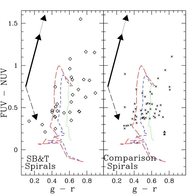
Figure 18: The GALEX FUV $-$ NUV vs. g $-$ r colors for the main disks of the interacting galaxy sample classified by NED as S0/a $-$ Sd (left panel; open diamonds), compared to the spirals in the comparison sample (right panel; crosses). Solar metallicity zero-extinction synthesis models are superimposed, consisting of a typical spiral galaxy (see text) plus an instantaneous burst. The dotted and dashed curves mark models of constant burst strength but increasing age, starting with 10⁶ years at the bottom of the page. Three burst strengths are plotted, with f_z(young)/f_z(old) = 0.01 (green dotted), 0.1 (blue short dashed), and 0.2 (red long dashes). All models include H$\alpha$ but no other emission lines. The sharp bend in the models to red g $-$ r colors at young ages is due to contributions from H$\alpha$. The three arrows show reddening vectors as described in the text.

To explain these differences, we made some simple comparisons with population synthesis models. In Figures 18 $-$ 22, we again display the various color-color plots for the two spiral samples. On these plots, we have superimposed evolutionary tracks from version 5.1 of the Starburst99 (SB99) population synthesis code (Leitherer et al., 1999). Following Larson & Tinsley (1978), in these models we have combined an underlying older stellar population with a burst of star formation. We calculated models with a range of ‘burst strengths’ f_z(young)/f_z(old) = 0.01 (green dotted curves), 0.1 (blue short dashed curves), and 0.2 (red long dashed curves), where f_z(young)/f_z(old) is the flux density in the z band due to the young stellar population, compared to that from the older stars. In Figures 18 $-$ 22, the plotted curves represent models with increasing burst age and constant burst strength. For the underlying older stellar population for these models, we have used moderately red colors that lie along the mean color curves for the comparison spiral sample, at FUV $-$ NUV = 0.75, NUV $-$ g = 2.6, u $-$ g = 1.3, g $-$ r = 0.6, r $-$ i = 0.27, and i $-$ z = 0.27. Thus we are assuming that the pre-interaction galaxies are typical star-forming spiral galaxies which have undergone an additional burst of star formation due to the interaction. We note that if the assumed underlying population is different than these nominal values, the general shape of the curves in Figures 18 $-$ 22 will remain the same, but they will be shifted to the new endpoint and the curves will be compressed, for a blueward shift of the underlying population, or stretched out for a redward shift.

For these models, we have assumed an instantaneous burst, solar metallicity, Kroupa (2002) initial mass functions (IMF), and an initial mass range of 0.1 $-$ 100 M${}_{\hbox{$\odot$}}$. This version of the SB99 code includes the Padova asymptotic giant-branch stellar models (Vázquez & Leitherer, 2005). We calculated model colors for a series of ages starting at 1 Myrs, increasing by step sizes of 1 Myr to 20 Myrs, then by 5 Myr steps to 50 Myrs, then 10 Myr steps to 100 Myrs. For all models, we included the nebular continuum from SB99. As in Smith et al. (2008, 2010), we also added the H$\alpha$ line to the model flux for the r band filter. For very young bursts (1 $-$ 5 Myrs), the r magnitude will decrease by 1.1 $-$ 0.25 magnitudes due to H$\alpha$, causing a sudden ‘bend’ in the model curves to redder g $-$ r at young ages. This bend is visible in the FUV $-$ NUV vs. g $-$ r plot (Figure 18), at young burst ages. For the calculations of the H$\alpha$ contributions, we used the redshift of Arp 285, which is typical of the SB&T sample. For the highest redshift galaxies in our sample, this will be an over-estimate, as H$\alpha$ will be redshifted to a less sensitive portion of the r band response function. Note that our models do not include the [O III] $\lambda$5007 or H$\beta$ line, which can contribute substantially to the g filter for low metallicity young galaxies (e.g., Krüger, Fritze-Alvensleben, & Loose, 1995; West et al., 2009), thus partially counteracting the reddening trend in g $-$ r.

In Figures 18 $-$ 22, we have also included arrows showing some possible reddening vectors due to dust. The amount of reddening in each band depends upon the type of dust and the geometry of the system, and can differ quite a bit depending upon the assumptions made. To illustrate the range in possible reddening models, on these plots we have included three example reddening vectors from the multiple-scattering radiative transfer calculations of Witt & Gordon (2000). In all three models plotted, the length of the vector plotted corresponds to ${\tau}_{\rm V}$ = 1. The solid arrow corresponds to a model with a smooth distribution of Small Magellanic Cloud-like dust evenly mixed amongst the stars. The dashed arrow corresponds to clumpy Milky Way-like dust mixed with the stars. The dotted arrow is produced by clumpy SMC dust distributed in a shell outside of the stars. See Witt & Gordon (2000) for more information about these models.

We recognize that the simple population synthesis models plotted in Figures 18 $-$ 22 do not accurately represent the true star formation histories of these galaxies. First, the older stellar population likely varies from galaxy to galaxy, which will shift the location of the model curves shown in Figure 18 $-$ 22. Second, the young stellar population may not be best represented by an single instantaneous burst. Also, the geometry of the system is likely more complex than in these simple reddening models, and the extinction may be different for the young and old stellar populations. However, these models are still valuable for illustrating some general trends. Our goal is not to provide accurate star formation histories for individual galaxies in the two samples, but simply to look for trends that will help in interpreting the differences between the two samples.

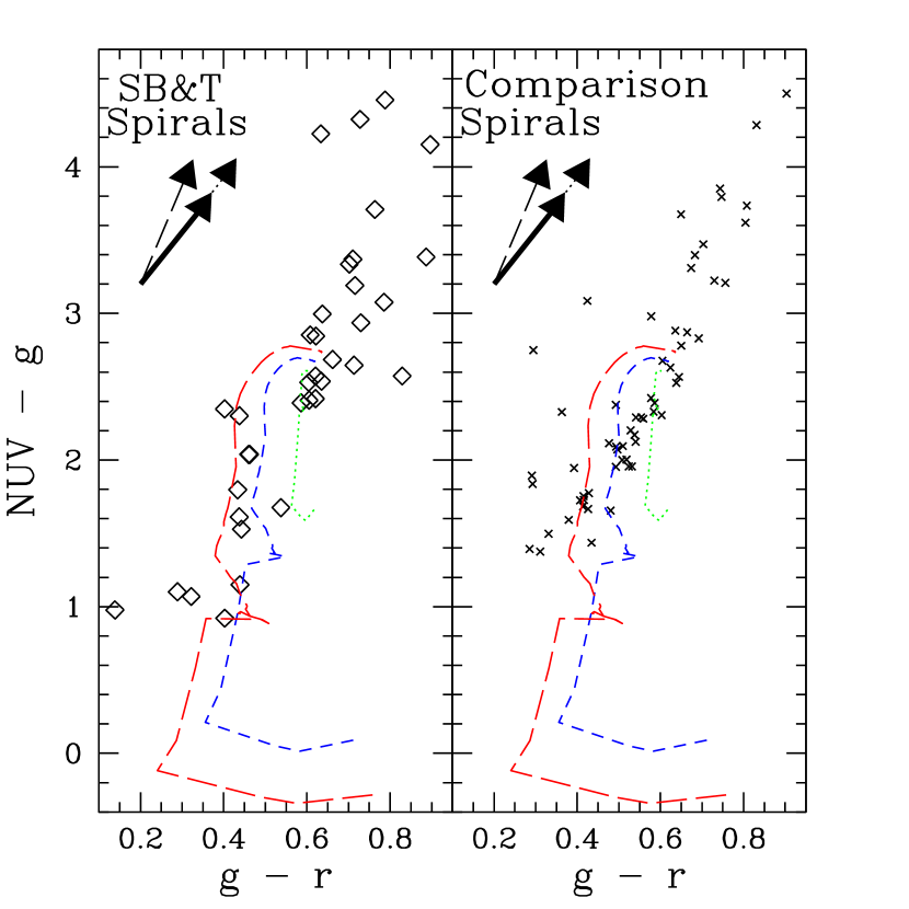
Figure 19: The GALEX NUV $-$ g vs. g $-$ r colors for the main disks of the interacting galaxy sample classified by NED as S0/a $-$ Sd (left panel; open diamonds), compared to the spirals in the comparison sample (right panel; crosses). Solar metallicity zero-extinction synthesis models are superimposed, consisting of a typical spiral galaxy (see text) plus an instantaneous burst. The dotted and dashed curves mark models of constant burst strength but increasing age, starting with 10⁶ years at the bottom of the page. Three burst strengths are plotted, with f_z(young)/f_z(old) of 0.01 (green dotted), 0.1 (blue short dashed), and 0.2 (red long dashes). All models include H$\alpha$ but no other emission lines. The three arrows show reddening vectors as described in the text.

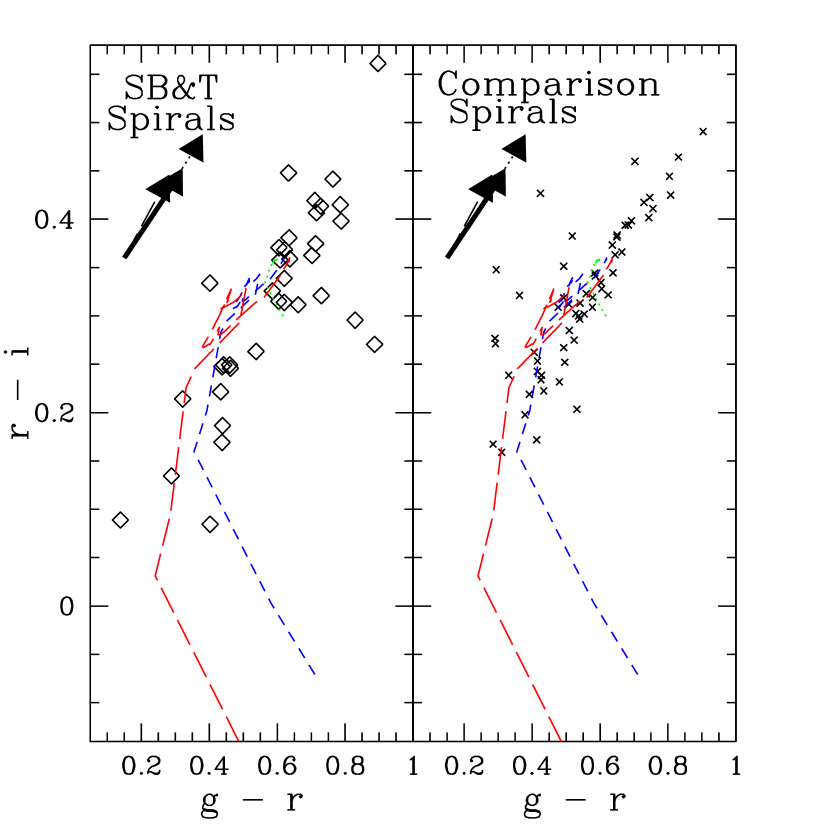
Figure 21: The GALEX g $-$ r vs. r $-$ i colors for the main disks of the interacting galaxy sample classified by NED as S0/a $-$ Sd (open diamonds), compared to the spirals in the comparison sample (crosses). Solar metallicity zero-extinction synthesis models are superimposed, consisting of a typical spiral galaxy (see text) plus an instantaneous burst. The dotted and dashed curves mark models of constant burst strength but increasing age, starting with 10⁶ years at the bottom of the page. Three burst strengths are plotted, with f_z(young)/f_z(old) of 0.01 (green dotted), 0.1 (blue short dashed), and 0.2 (red long dashes). The three arrows show reddening vectors as described in the text.

In all of these color-color plots, some degeneracy between age and extinction is visible, as seen by a comparison of the burst models and the extinction vectors. When bursts of different strengths are added to the older stellar population, the models shift in characteristic ways in the color-color plots. For relatively young bursts, the FUV and NUV bands are dominated by light from the burst. In contrast, the i and z optical bands are predominantly light from the older stars. The u, g, and r bands have important contributions from both, with the proportions varying with burst strength and age. In the FUV $-$ NUV vs. g $-$ r diagram (Figure 18), increasing burst strength causes a shift in g $-$ r towards the blue. In this plot, the age and burst strength vectors point in different directions. In the NUV $-$ g vs. g $-$ r plot (Figure 19), increasing the burst strength also causes a shift at an angle to the direction of increasing burst age. In contrast, in the two longer wavelength optical plots (Figures 21 $-$ 22), increasing the burst strength shifts both colors bluewards, and the direction of increasing burst strength is approximately parallel to the age vector, and roughly anti-parallel with the extinction vector. Thus there is more degeneracy in these two plots.

In the shorter wavelength plots, the main difference between the two samples is the less concentrated distribution of points in the interacting galaxy sample, without a strong difference in the medians of the colors for the two samples. Stronger bursts alone would tend to shift the medians to bluer colors, while larger extinctions alone would shift the medians to the red. The lack of a pronounced systematic shift in colors between the two samples suggests that, on average, the interacting sample has both stronger ‘bursts’ in some galaxies (i.e., higher current rates of star formation), and larger extinctions in others. These two effects together will tend to spread out the distribution of colors in the observed manner (see Figure 18).

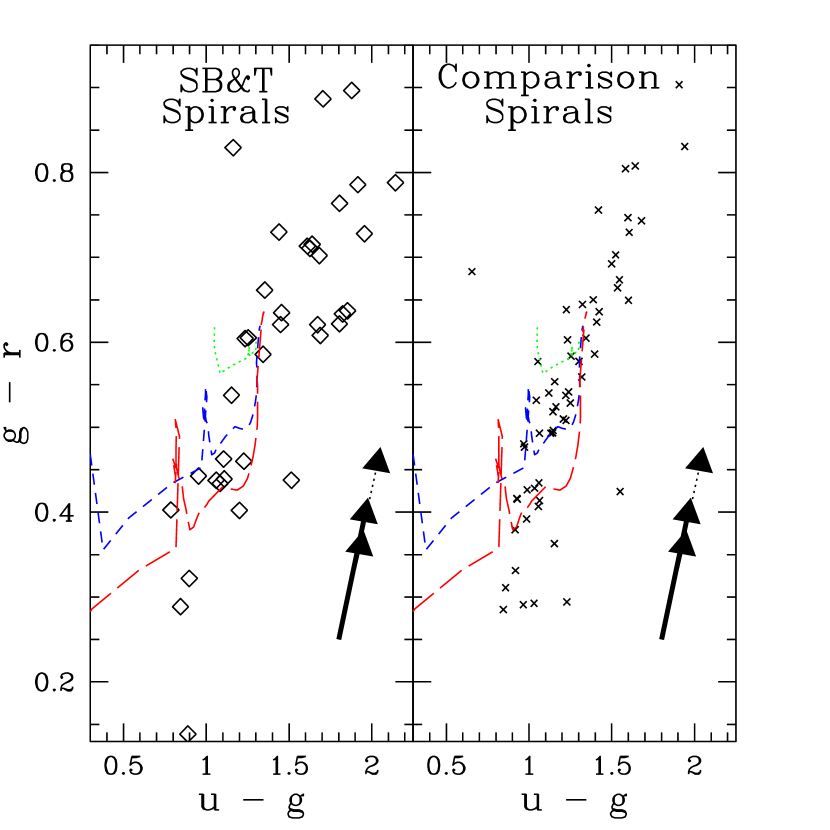
Figure 20: The GALEX u $-$ g vs. g $-$ r colors for the main disks of the interacting galaxy sample classified by NED as S0/a $-$ Sd (open diamonds), compared to the spirals in the comparison sample (crosses). Solar metallicity zero-extinction synthesis models are superimposed, consisting of a typical spiral galaxy (see text) plus an instantaneous burst. The dotted and dashed curves mark models of constant burst strength but increasing age, starting with 10⁶ years at the bottom of the page. Three burst strengths are plotted, with f_z(young)/f_z(old) of 0.01 (green dotted), 0.1 (blue short dashed), and 0.2 (red long dashes). All models include H$\alpha$ but no other emission lines. The three arrows show reddening vectors as described in the text.

As noted earlier, in the NUV $-$ g vs. g $-$ r plot (Figure 8), there is a slight shift to bluer NUV $-$ g for a given g $-$ r for the interacting galaxies, in addition to larger scatter. This could be accounted for by the combined effect of some galaxies having stronger bursts, and other galaxies having stronger extinctions (see Figure 19). In the u $-$ g vs. g $-$ r plot (Figure 9), there is a shift to bluer g $-$ r values for a given u $-$ g value (or equivalently, a reddening of u $-$ g for a given g $-$ r). A shift in that direction can be produced by stronger bursts (Figure 20), on average, for the interacting galaxies. However, to explain the reddest colors in this plot requires some of the interacting galaxies to have more extinction, on average, compared to the comparison sample.

Thus we conclude that the interacting galaxies, on average, have both stronger bursts compared to the comparison sample, and higher average extinctions. However, there are strong variations across the sample in both burst strength and in extinction. This is consistent with earlier studies based on H$\alpha$ and far-infrared observations (Kennicutt et al., 1987; Bushouse, 1987; Bushouse, Lamb, & Werner, 1988), which showed that the enhancement in the star formation rate of interacting galaxies is an average effect; some interacting galaxies show no enhancement at all.

Our conclusion that the interacting galaxies tend to have stronger extinction on average is consistent with earlier studies which found that the star formation in interacting galaxies tends to be more centrally concentrated than in normal spirals (Bushouse, 1987; Smith et al., 2007). Numerical models suggest that interactions can drive gas into the central regions of galaxies, triggering central starbursts. This central concentration may lead to larger extinction on average in the interacting sample. In support of this idea, Bushouse (1987) and Bushouse, Lamb, & Werner (1988) found higher L_FIR/L_Hα ratios in their interacting sample compared to spirals, also suggesting more obscured star formation on average.

In addition to age, extinction, and burst strength variations, other factors that can cause scatter in the observed color-color diagrams are galaxy-to-galaxy variations in the IMF, the metallicity, the properties of the dust, particularly the dust attenuation law, and the spatial distribution of the dust relative to the stars, including the clumpiness of the dust. The relative importance of these factors to the observed colors of galaxies is discussed in detail by Conroy, White, & Gunn (2010a, b). A clumpier dust distribution will tend to make the observed colors bluer, while a steeper IMF will redden the colors. At the present time, however, there is no strong evidence of significant differences between the two samples in any of these parameters.

12 Summary

We have compared the UV/optical colors of a well-defined sample of pre-merger interacting galaxy pairs with those of ‘normal spirals’. As previously found for optical colors alone by Larson & Tinsley (1978), the interacting galaxies show a larger dispersion in their colors compared to the normal spirals. This effect is especially pronounced in the shorter wavelength UV/optical colors, due to the increased sensitivity to both young stars and dust. This increased scatter is best explained by a combination of both moderately-enhanced star formation in the interacting galaxies, along with larger average extinction. In interacting systems, gas may be driven into the central regions of the galaxies, triggering star formation while at the same time increasing the average column density of dust. While massive young stars are blue, they tend to be reddened by heavy layers of dust, thus interacting galaxies are not dramatically bluer on average than non-interacting systems. However, the dust screens are known to be irregular or fractal, so some very blue light can escape. These combined effects tend to increase the scatter in the observed UV/optical colors of interacting systems.

Our multi-wavelength database for both the SB&T sample and the ‘normal’ spiral galaxies should prove useful for future comparisons with other galaxy samples such as cluster spirals and spirals in compact groups, to investigate star formation enhancement in these environments. Both samples should also be useful for comparison with high redshift galaxies.

Figure 1: The distribution of distances for the galaxies in the two samples.

Figure 2: The distribution of Galactic latitudes for the two samples.

Figure 3: The number of neighbors per galaxy in each sample, when a neighbor is defined as being within 2 Mpc and $\delta$V $\leq$ 1000 km s^-1, with an absolute V magnitude brighter than $-$18.5.

Figure 4: The distribution of morphological types of the two samples, as well as that used for the type-matched subsets of the comparison sample. See text for more information.

Figure 5: A comparison of the distributions of NUV luminosities for the full comparison sample (bottom panel), the full SB&T sample (top panel), the SB&T spiral-only sample (second panel), the tails and bridges (third panel), and the candidate tidal dwarf galaxies (fourth panel). The hatched regions are upper limits.

Figure 6: A comparison of the distributions of g luminosities for the full comparison sample (bottom panel), the full SB&T sample (top panel), the SB&T spiral-only sample (second panel), the tails and bridges (third panel), and the candidate tidal dwarf galaxies (fourth panel). The hatched regions are upper limits.

Figure 7: The GALEX FUV $-$ NUV vs. g $-$ r colors for the main disks of the interacting galaxy sample classified by NED as S0/a $-$ Sd (left panel; open diamonds), compared to the spirals in the full comparison sample (right panel; crosses). The solid line shows the mean values of g $-$ r for the full comparison sample calculated in 0.1 magnitude bins of FUV $-$ NUV, while the dotted line gives the mean values for the SB&T spirals. The mean statistical uncertainties for the datapoints are plotted in the lower left.

Figure 8: The GALEX NUV $-$ g vs. g $-$ r colors for the main disks of the interacting galaxy sample classified by NED as S0/a $-$ Sd (left panel; open diamonds), compared to the spirals in the full comparison sample (right panel; crosses). The solid line shows the mean values of g $-$ r for the full comparison sample calculated in 0.2 magnitude bins of NUV $-$ g, while the dotted line gives the mean values for the SB&T spirals. The mean statistical uncertainties are plotted in the lower left.

Figure 9: The GALEX u $-$ g vs. g $-$ r colors for the main disks of the interacting galaxy sample classified by NED as S0/a $-$ Sd (open diamonds), compared to the spirals in the full comparison sample (crosses). The solid line shows the mean values of u $-$ g for the comparison sample calculated in 0.1 magnitude bins of g $-$ r, while the dotted line gives the mean values for the SB&T spirals. The mean statistical uncertainties are plotted in the lower left.

Figure 10: The GALEX g $-$ r vs. r $-$ i colors for the main disks of the interacting galaxy sample classified by NED as S0/a $-$ Sd (open diamonds), compared to the spirals in the full comparison sample (crosses). The solid line shows the mean values of g $-$ r for the comparison sample calculated in 0.1 magnitude bins of r $-$ i, while the dotted line gives the mean values for the SB&T spirals. The mean statistical uncertainties are plotted in the lower left.

Figure 11: The GALEX r $-$ i vs. i $-$ z colors for the main disks of the interacting galaxy sample classified by NED as S0/a $-$ Sd (open diamonds), compared to the spirals in the full comparison sample (crosses). The solid line shows the mean values of r $-$ i for the comparison sample calculated in 0.1 magnitude bins of i $-$ z, while the dotted line gives the mean values for the SB&T spirals. The mean statistical uncertainties are plotted in the lower left.

Figure 12: Plots of FUV $-$ NUV color vs. morphological type for the SB&T sample and the full comparison sample. The solid lines show the mean-value line for types Sa $-$ Sd for the comparison spirals, while the dotted line marks the mean-value curve for the interacting sample. Statistical uncertainties are shown.

Figure 13: Plots of NUV $-$ g color vs. morphological type for the SB&T sample and the full comparison sample. The solid lines show the mean-value line for types Sa $-$ Sd for the comparison spirals, while the dotted line marks the mean-value curve for the interacting sample. Statistical uncertainties are shown.

Figure 14: Plots of u $-$ g color vs. morphological type for the SB&T sample and the full comparison sample. The solid lines show the mean-value line for types Sa $-$ Sd for the comparison spirals, while the dotted line marks the mean-value curve for the interacting sample. Statistical uncertainties are shown.

Figure 15: Plots of g $-$ r color vs. morphological type for the SB&T sample and the full comparison sample. The solid lines show the mean-value line for types Sa $-$ Sd for the comparison spirals, while the dotted line marks the mean-value curve for the interacting sample. Statistical uncertainties are shown.

Figure 16: Plots of r $-$ i color vs. morphological type for the SB&T sample and the full comparison sample. The solid lines show the mean-value line for types Sa $-$ Sd for the comparison spirals, while the dotted line marks the mean-value relation for the interacting sample. Statistical uncertainties are shown.

Figure 17: Plots of i $-$ z color vs. morphological type for the SB&T sample and the full comparison sample. The solid lines show the mean-value line for types Sa $-$ Sd for the comparison spirals, while the dotted line marks the mean-value relation for the interacting sample. Statistical uncertainties are shown.

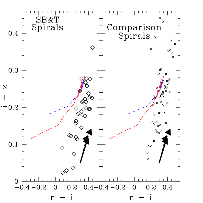
Figure 22: The GALEX r $-$ i vs. i $-$ z colors for the main disks of the interacting galaxy sample classified by NED as S0/a $-$ Sd (open diamonds), compared to the spirals in the comparison sample (crosses). Solar metallicity zero-extinction synthesis models are superimposed, consisting of a typical spiral galaxy (see text) plus an instantaneous burst. The dotted and dashed curves mark models of constant burst strength but increasing age, starting with 10⁶ years at the bottom of the page. Three burst strengths are plotted, with f_z(young)/f_z(old) of 0.01 (green dotted), 0.1 (blue short dashed), and 0.2 (red long dashes). All models include H$\alpha$ but no other emission lines. At these wavelengths, the three reddening vectors are very similar.

Table 1: Optical and UV Magnitudes for Normal Spiral Galaxy Sample^a

	FUV	NUV	u	g	r	i	z
Name	(mag)	(mag)	(mag)	(mag)	(mag)	(mag)	(mag)
CGCG 0377-039	17.86 $\pm$ 0.09	17.34 $\pm$ 0.01	15.91 $\pm$ 0.05	14.49 $\pm$ 0.01	13.85 $\pm$ 0.01	13.47 $\pm$ 0.01	13.26 $\pm$ 0.01
IC 0159	15.89 $\pm$ 0.00	15.48 $\pm$ 0.00	14.86 $\pm$ 0.04	13.80 $\pm$ 0.01	13.39 $\pm$ 0.01	13.21 $\pm$ 0.03	13.14 $\pm$ 0.03
IC 0653	$\geq$17.38	17.20 $\pm$ 0.03	15.01 $\pm$ 0.07	13.41 $\pm$ 0.01	12.66 $\pm$ 0.01	12.24 $\pm$ 0.01	12.00 $\pm$ 0.01
IC 0673	16.35 $\pm$ 0.03	15.92 $\pm$ 0.02	14.99 $\pm$ 0.16	13.85 $\pm$ 0.03	13.34 $\pm$ 0.03	13.04 $\pm$ 0.05	12.89 $\pm$ 0.13
IC 0716	18.02 $\pm$ 0.10	17.63 $\pm$ 0.05	16.02 $\pm$ 0.06	14.41 $\pm$ 0.01	13.68 $\pm$ 0.01	13.26 $\pm$ 0.01	13.01 $\pm$ 0.04
IC 0952	16.88 $\pm$ 0.05	16.45 $\pm$ 0.00	15.40 $\pm$ 0.04	14.16 $\pm$ 0.00	13.62 $\pm$ 0.00	13.31 $\pm$ 0.01	13.10 $\pm$ 0.01
IC 1221	15.38 $\pm$ 0.00	15.30 $\pm$ 0.00	14.93 $\pm$ 0.03	13.87 $\pm$ 0.01	13.43 $\pm$ 0.02	13.21 $\pm$ 0.03	13.02 $\pm$ 0.07
IC 1222	16.23 $\pm$ 0.03	15.76 $\pm$ 0.00	14.81 $\pm$ 0.03	13.56 $\pm$ 0.00	13.03 $\pm$ 0.00	12.73 $\pm$ 0.01	12.56 $\pm$ 0.02
IC 3467	17.54 $\pm$ 0.35	17.00 $\pm$ 0.02	16.32 $\pm$ 0.12	15.20 $\pm$ 0.03	14.82 $\pm$ 0.04	14.53 $\pm$ 0.03	14.36 $\pm$ 0.07
IC 4229	16.46 $\pm$ 0.03	15.83 $\pm$ 0.00	15.04 $\pm$ 0.02	13.88 $\pm$ 0.01	13.35 $\pm$ 0.01	13.08 $\pm$ 0.01	12.85 $\pm$ 0.02

Table 2: RMS Deviations for the Color-Color Plots^a

Colors	Full	Mean	SB&T	SB&T
	Comparison	Type-Matched	Spirals	Spirals
	Sample	Subsets	vs.	vs.
			own mean	comp. mean
FUV $-$ NUV vs. g $-$ r	0.111	0.108	0.128	0.156
NUV $-$ g vs. g $-$ r	0.065	0.060	0.079	0.123
g $-$ r vs. u $-$ g	0.124	0.120	0.216	0.286
r $-$ i vs. g $-$ r	0.090	0.087	0.106	0.117
i $-$ z vs. r $-$ i	0.076	0.063	0.062	0.071

Table 3: RMS Deviations for Color vs. Type Plots^a

Color	Full	Mean	SB&T
	Comparison	Type-Matched	Spiral
	Sample	Subsets	Sampleb
FUV $-$ NUV	0.200	0.194	0.302
NUV $-$ g	0.527	0.557	0.811
u $-$ g	0.194	0.201	0.310
g $-$ r	0.120	0.123	0.118
r $-$ i	0.074	0.073	0.079
i $-$ z	0.090	0.081	0.061

References

- Abazajian et al. (2003) Abazajian, K., et al. 2003, AJ, 126, 2081
- Abraham et al. (1996) Abraham, R. G., van den Bergh, S., Glazebrook, K., Ellis, R. S., Santiago, B. X., Surma, P., & Griffiths, R. E. 1996, ApJS, 107, 1
- Arp (1966) Arp, H. 1966, Atlas of Peculiar Galaxies (Pasadena: Caltech)
- Barton et al. (2000) Barton, E. J., Geller, M. J., & Kenyon, S. J. 2000, ApJ, 530, 660
- Barton Gillespie, Geller, & Kenyon (2003) Barton Gillespie, E., Geller, M. J., & Kenyon, S. J. 2003, ApJ, 582, 668
- Barton et al. (2007) Barton, E. J., Arnold, J. A., Zentner, A. R., Bullock, J. S., and Wechsler, R. H. 2007, ApJ, 671, 1538
- Bergvall, Laurikainen, & Aalto (2003) Bergvall, N., Laurikainen, E. & Aalto, S. 2003, A&A 405, 31
- Boissier et al. (2007) Boissier, S., et al. 2007, ApJS, 173, 524
- Boselli et al. (2005) Boselli, A., et al. 2005, ApJ, 623, L13
- Boselli et al. (2010) Boselli, A., et al. 2010, PASP, 122, 261
- Bushouse (1987) Bushouse, H. A. 1987, ApJ, 320, 49
- Bushouse, Lamb, & Werner (1988) Bushouse, H. A., Lamb, S. A., & Werner, M. W. 1988, ApJ, 335, 74
- Cardelli, Clayton, & Mathis (1989) Cardelli, J. A., Clayton, G. C., & Mathis, J. S. 1989, ApJ, 345, 245
- Conroy, White, & Gunn (2010a) Conroy, C., White, M., & Gunn, J. E. 2010a, ApJ, 708, 58
- Conroy, White, & Gunn (2010b) Conroy, C., White, M., & Gunn, J. E. 2010b, ApJ, 712, 833
- de Vaucouleurs, de Vaucouleurs, & Corwin (1976) de Vaucouleurs, G., de Vaucouleurs, A., & Corwin, H. G. 1976, Second Reference Catalogue of Bright Galaxies (Austin: University of Texas Press) (RC2).
- de Vaucouleurs (1977) de Vaucouleurs, G. 1977, in the Proceedings of ‘The Evolution of Galaxies and Stellar Populations’, eds. B. M. Tinsley and R. B. Larson (New Haven: Yale University Observatory).
- Gil de Paz et al. (2005) Gil de Paz, A., et al. 2005, ApJ, 627, L29
- Gil de Paz et al. (2007) Gil de Paz, A., et al. 2007, ApJS, 173, 185
- Gómez et al. (2003) Gómez, P. L., et al. 2003, ApJ, 584, 210
- Hancock et al. (2007) Hancock, M., Smith, B. J., Struck, C., Giroux, M. L., Appleton, P. N., Charmandaris, V., & Reach, W. T. 2007, AJ, 133, 791
- Hancock et al. (2009) Hancock, M., Smith, B. J., Struck, C., Giroux, M. L, & Hurlock, S. 2009, AJ, 137, 4643
- Keel (2010) Keel, W. C. 2010, Proceedings of the ‘Galaxy Wars: Stellar Populations and Star Formation in Interacting Galaxies’ conference, Astronomical Society of the Pacific Conference Series, Volume 423, 249
- Kennicutt et al. (2003) Kennicutt, R. C., Jr., et al. 2003, PASP, 115, 928
- Kennicutt et al. (1987) Kennicutt, R. C., Jr., Keel, W. C., van der Hulst, J. M., Hummel, E., & Roettiger, K. A. 1987, AJ, 93, 1011
- Kroupa (2002) Kroupa, P. 2002, Science, 295, 85
- Krüger, Fritze-Alvensleben, & Loose (1995) Krüger, H., Fritz-v. Alvensleben, U., & Loose, H.-H. 1995, A&A, 303, 41
- Lambas et al. (2003) Lambas, D. G., Tissera, P. B., Alonso, M. S., & Coldwell, G. 2003, MNRAS, 346, 1189
- Larson & Tinsley (1978) Larson, R. B. & Tinsley, B. M. 1978, ApJ, 219, 46
- Leitherer et al. (1999) Leitherer, C., et al. 1999, ApJS, 123, 3
- Li et al. (2008) Li, C., Kauffmann, G., Heckman, T. M., Jing, Y. P., & White, S. D. 2008, MNRAS, 385, 1903
- Lotz et al. (2006) Lotz, J. M., Madau, P., Giavalisco, M., Primack, J., & Ferguson, H. C. 2006, ApJ, 636, 592
- Martin et al. (2005) Martin, D. C., et al. 2005, ApJ, 619, L1
- Mñoz-Mateos et al. (2009) Muñoz-Mateos, J. C., et al. 2009, ApJ, 703, 1569
- Neff et al. (2005) Neff, S. G., et al. 2005, ApJ, 619, L91
- Nikolic, Cullen, & Alexander (2004) Nikolic, B., Cullen, H., & Alexander, P. 2004, MNRAS, 355, 874
- Overzier et al. (2008) Overzier, R. A., et al. 2008, ApJ, 677, 37
- Peterson et al. (2009) Peterson, B. W., Struck, C., Smith, B. J., & Hancock, M. 2009, MNRAS, 400, 1208
- Petty et al. (2009) Petty, S. M., de Mello, D. F., Gallagher, J. S., Gardner, J. P., Lotz, J. M., Matt Mountain, C., & Smith, L. J. 2009, AJ, 138, 362
- Sandage (1961) Sandage, A. 1961, The Hubble Atlas of Galaxies (Washington D.C.: Carnegie Institute of Washington).
- Schlegel, Finkbeiner, & Davis (1998) Schlegel, D. J., Finkbeiner, D. P., & Davis, M. 1998, ApJ, 500, 525
- Schombert, Wallin, & Struck-Marcell (1990) Schombert, J. M., Wallin, J. F., & Struck-Marcell, C. 1990, AJ, 99, 497
- Schweizer (1978) Schweizer, F. 1978, in Structure and Properties of Nearby Galaxies, ed. E. M. Berkhuijsen & R. Wielebinski (Dordrecht: Reidel), 279
- Smith et al. (2008) Smith, B. J., et al. 2008, AJ, 135, 2406
- Smith et al. (2010) Smith, B. J., Giroux, M. L., Struck, C., Hancock, M., & Hurlock, S. 2010, AJ, 139, 1212; Erratum 2010, AJ, 139, 1212.
- Smith et al. (2007) Smith, B. J., Struck, C., Hancock, M., Appleton, P. N., Charmandaris, V., & Reach, W. T. 2007, AJ, 133, 791
- Smith et al. (2005) Smith, B. J., Struck, C., Appleton, P. N., Charmandaris, V., Reach, W., & Eitter, J. J. 2005, AJ, 130, 2117
- Sol Alonso et al. (2006) Sol Alonso, M., Lambas, D. G., Tissera, P., & Coldwell, G. 2006, MNRAS, 367, 1029
- Struck-Marcell & Tinsley (1978) Struck-Marcell, C. & Tinsley, B. M. 1978, ApJ, 221, 562
- Struck & Smith (2003) Struck, C. & Smith, B. J. 2003, ApJ, 589, 157
- Vázquez & Leitherer (2005) Vázquez, G. A. & Leitherer, C. 2005, ApJ, 621, 695
- Thilker et al. (2005a) Thilker, D. A., et al. 2005a, ApJ, 619, L67
- Thilker et al. (2005b) Thilker, D. A., et al. 2005b, ApJ, 619, L79
- West et al. (2009) West, A. W., Garcia-Appadoo, D. A., Dalcanton, J. J., Disney, M. J., Rockosi, C. M., & Ivezić, Z. 2009, AJ, 138, 796
- Witt & Gordon (2000) Witt, A. N. & Gordon, K. D. 2000, ApJ, 463, 681