Anisotropic surface transport in topological insulators in proximity to a helical spin density wave

Abstract

We study the effects of spatially localized breakdown of time reversal symmetry on the surface of a topological insulator (TI) due to proximity to a helical spin density wave (HSDW). The HSDW acts like an externally applied one-dimensional periodic(magnetic) potential for the spins on the surface of the TI, rendering the Dirac cone on the TI surface highly anisotropic. The decrease of group velocity along the direction $\hat{x}$ of the applied spin potential is twice as much as that perpendicular to $\hat{x}$. At the Brillouin zone boundaries (BZB) it also gives rise to new semi-Dirac points which have linear dispersion along $\hat{x}$ but quadratic dispersion perpendicular to $\hat{x}$. The group velocity of electrons at these new semi-Dirac points is also shown to be highly anisotropic. Experiments using TI systems on multiferroic substrates should realize our predictions. We further discuss the effects of other forms of spin density wave on the surface transport property of topological insulator.

I Introduction

In the last few years there has been a growing interest in topological insulators (TI), which are materials that are insulators in the bulk but conduct two-dimensionally on the surfaces Qi et al. (2008); Hsieh et al. (2009); Zhang et al. (2009a); Roy (2009); Chen et al. (2009); Hasan and L. . The non-trivial topology of the wavefunction of such TI has been predicted to show metallic surface conductivity that is topologically protected against weak disorder and interaction effects. One of the mechanisms by which the surface modes can be disrupted is by breaking the time reversal invariance upon applying a magnetic field. There have been several studies on the effects of a magnetic field either applied directly perpendicular to the surface of a TI Tse and MacDonald (2010) or by the proximity effect of a ferromagnet in a heterostructure Mondal et al. (2010); Garate and Franz (2010). On the other hand, the effects of an antiferromagnet or a spin density wave on the surface states of the TI is a topic which is much less well-explored. We carry out such an analysis of the effect of a spin density wave on TI transport in this work.

Although an antiferromagnet, in the proximity to a TI, does not affect the global time reversal symmetry (TRS) in the latter, the staggered nature of the spins in the antiferromagnet breaks the TRS locally. In this work, we are interested in how this local TRS breaking affects the surface states of the TI. However, the local TRS breaking occurs at a length scale which is of the order of the lattice spacing in the antiferromagnet (for e.g., $8.85\AA$ for MnO). Therefore the effects of local TRS breaking occur at very large momenta, which makes it difficult to observe them in experiments. In order to redress this difficulty, we propose to study the effects of local TRS breaking by replacing the antiferromagnet with a multiferroic materialCheong and Mostovoy (2007) like orthorhombic RMnO₃ (R being a rare earth element like Tb or Dy) or the family of Fe_1-xCo_xSi with cubic but noncentrosymmetric structure, which shows a helical spin density wave (HSDW) order with relatively long periods ($>30$nm) Uchida et al. (2006). The HSDW will couple to the Dirac fermions on the surface of the topological insulator due to the proximity effect by the above two kinds of materials directly deposited on the top. The situation is similar to that of an externally applied charge potential on graphene Park et al. (2008). However, the contrast between the two situations is that the 3D topological insulator has spin polarized 2D Dirac fermions on its surface Xia et al. (2009), whereas the Dirac fermions in graphene carry pseudo-spin. Nevertheless, in analogy with the charge potential applied to graphene, a spin potential can be used for TI to manipulate the surface Dirac fermions.

It may be appropriate to ask about the motivation of our theoretical work where we are proposing, using concrete theoretical calculations, that experiments be carried out on a multiferroic-TI sandwich structure for the observation of the topologically protected surface transport in the TI surface states induced by the HSDW associated with the multiferroic layer. This approach sounds somewhat indirect, and indeed it is although the effect of the HSDW-induced local TRS-breaking on TI surface transport properties is intrinsically interesting in its own right as we establish in this work.

Our main motivation for this work, however, arises from the fact that so far there has been little direct experimental signature of the topologically-protected surface transport in existing TI materials in spite of a great deal of research activity Ren et al. (2010); Qu et al. (2010); Butch et al. (2010); Analytis et al. (2010); Culcer et al. (2010); Checkelsky et al. ; Taskin et al. (2010); Nishide et al. (2010); Eto et al. (2010) aimed precisely toward the direct and unambiguous observation of 2D surface TI transport. All the convincing experimental evidence for the existence of the topologically-protected surface 2D TI states is currently based on the verification of the proposed band structure through STM/STS or ARPES type spectroscopic measurements. The problem in the direct observation of the surface 2D TI transport is that the currently existing TI materials are not good bulk insulators, and the bulk conduction is always much stronger than the surface conduction, making it impossible to observe the surface 2D states unambiguously in transport measurements. This problem of substantial bulk transport arises from the fact that all existing TI materials, instead of being a bulk band insulator as band structure calculations predict, turn out to be intrinsically doped in the bulk due to defects and vacancies, giving rise to a large bulk conduction channel which competes directly with the surface 2D transport. For example, the two most recent (and also most compelling) transport measurements Ren et al. (2010); Qu et al. (2010) see very small putative surface 2D magneto-resistance oscillations with a temperature dependent bulk resistivity which does not behave like a standard band insulator at all. In particular, the bulk resistivity in these samples Ren et al. (2010); Qu et al. (2010) is of the order of $\Omega\cdot$cm or less whereas an insulator typically has a bulk resistivity which is 10–12 orders of magnitude larger. Thus, the TI systems, even in these most compelling measurements, show dominant bulk conduction with less than 1% of the net conduction being inferred (through the indirect fitting of the magneto-resistance data using many free parameters and ad hoc multichannel conduction models) at best to be arising from the 2D surface states. Another recent experiment Butch et al. (2010) concludes that no 2D surface conduction can be discerned at all in the TI transport data because of the dominant bulk conduction. Another recent experiment Analytis et al. (2010) goes to the extreme of using a pulsed external magnetic field as high as 55T in order to investigate the surface 2D transport, again emphasizing small observed features in the high-field resistivity as the possible manifestation of the expected 2D TI surface transport. Even the two very recent transport measurements Ren et al. (2010); Qu et al. (2010) purportedly claiming the manifestation of 2D surface TI transport can only observe small 2D features in the derivative spectrum of the resistivity with respect to the applied magnetic field. This is a most unsatisfactory state of affairs in sharp contrast to the transport properties of well-established 2D quantum systems, e.g. graphene, where 2D transport behavior Sarma et al. without any bulk conduction problem whatsoever manifests itself in every possible transport measurement in a decisive manner, and one does not have to look for small features in the derivative spectrum. The current situation in TI physics is thus extremely problematic with all spectroscopic measurements providing reasonable verification of the expected spin-resolved 2D Dirac cone band structure on the TI surface whereas the fact that the bulk is not an insulator is making it essentially impossible to see the expected 2D protected surface transport. We point out in this context that the theoretical details of how the surface 2D TI transport would behave, had it not been contaminated by the unintentional bulk conduction problem plaguing the existing TI materials, are reasonably well-known in the literature Culcer et al. (2010).

Of course, further materials development in the existing TI systems leading to the effective suppression of the unintentional bulk doping or the discovery of completely new classes of TI materials where the bulk is a true insulator could solve this problem instantaneously, but until that happens, any idea which points toward the observation of surface TI transport should be welcome. It is somewhat of an embarrassment that in spite of the huge activity in TI research, a true Topological Insulator does not yet exist since the existing systems are not true bulk insulators due to the invariable presence of unintentional bulk doping. Our proposal in the current work should be seen in this light. We provide a method to directly isolate surface transport features in TI systems in proximity to a helical spin density wave as produced, for example, by a multiferroic material. Since bulk conduction should be relatively immune to the presence of the HSDW, whereas the surface TI conduction should be affected qualitatively as we show in this work, we believe that our predictions could help provide the unambiguous observation of the surface 2D TI transport properties. In addition, the coupling between the HSDW and the 2D TI states leads to nontrivial novel physics (e.g. the semi-Dirac points to be discussed below) which is intrinsically interesting in its own right.

We find that the surface states of the TI are significantly modified in the presence of the HSDW. The HSDW acts like an externally applied superlattice potential on the TI surface resulting in striking anisotropy of the Dirac cones and group velocity of the surface states. In particular, the group velocity along the direction of the superlattice is monotonically suppressed as a function of the lattice potential strength and its period. For the type of HSDW considered in Sec. II, which we call proper HSDW, Kataoka and Nakanishi (1981) (see below), we find that novel semi-Dirac points, whose low-energy characteristics are intermediate between Dirac (massless) and zero-gap (massive) semiconductors Banerjee et al. (2009); Pardo and Pickett (2009), show up on the BZB. In Sec. III, we discuss how the surface transport properties of the topological insulator changes when the forms of the spin density wave is changed. Section IV contains a summary and conclusions.

II The proper helical spin density wave

II.1 Dirac cone on the BZ center

We begin by writing down the effective Hamiltonian for the low-energy quasiparticles on the surface of a topological insulator as,

$$H_{0}({\bf k})=\hbar v_{F}(k_{x}\sigma_{x}+k_{y}\sigma_{y})$$ (1)

where $v_{F}\simeq 6.2\times 10^{5}$m/s is the Fermi velocity of Dirac fermions in Bi₂Se₃ Zhang et al. (2009b) and $\sigma_{i}$ are the Pauli matrices. The Hamiltonian in Eq. (1) is characterized by an energy spectrum $\varepsilon_{s,k}=s\hbar v_{F}k$ where $s=\pm 1$ is the band index, and eigenstates given by

$$\left<{\bf r}|s,{\bf k}\right>=\frac{1}{\sqrt{2}}e^{i{\bf k}\cdot{\bf r}}\left(\begin{array}[]{c}1\\ se^{i\theta_{{\bf k}}}\end{array}\right)\ ,$$ (2)

where $\theta_{\bf k}$ is the angle of vector ${\bf k}$ with respect to the $\hat{k}_{x}$ direction.

In the presence of the HSDW on top of a TI, depicted schematically in Fig. 1, the Hamiltonian (1) is modified Yokoyama et al. (2010) to: $H=H_{0}({\bf k})+U(x)$, where the potential $U(x)$ for the HSDW can be written as:

$$\begin{array}[]{l l }U(x)=U_{y}\sigma_{y}\cos(\dfrac{2\pi}{L}x)+U_{z}\sigma_{z}\sin(\dfrac{2\pi}{L}x),\end{array}$$ (3)

where $L$ is the spatial period of the potential, and $U_{y,z}$ are the amplitudes of the HSDWKataoka and Nakanishi (1981). For the case $U_{z}<U_{y}$, we find no gapless states on the BZB. On the other hand, for $U_{z}>U_{y}$, two Dirac points centered at $(\frac{\pi}{L},\pm K_{y})$ emerge on the BZB, which will be discussed in Sec. III. For the symmetric HSDW such that $U_{z}=U_{y}=U_{0}$, which we shall call proper HSDW, we find a single semi-Dirac point at $(k_{x},k_{y})=(\pm\dfrac{\pi}{L},0)$ (Fig. 3a). In this section, we shall focus on the case of a proper HSDW on TI.

In our calculation, we use the value of induced exchange field due to the magnetic proximity effect being $5\sim 50$ meVHaugen et al. (2008); Chakhalian et al. (2006), which has been taken to be a reasonable valueYokoyama et al. (2010). The exchange-induced potential $U(x)$ from the HSDW creates a periodic potential on the surface of the TI. The electronic eigenstates of such a Hamiltonian can be written using Bloch’s theorem as

$$\psi_{n\bm{k}}(\bm{r})=\sum_{\bm{G}}e^{i(\bm{k}+\bm{G})\cdot\bm{r}}c(n,\bm{k}+\bm{G})$$ (4)

where ${\bf G}=\dfrac{2m\pi}{L}\hat{x}$ ($m\in$ integer) is the reciprocal lattice vector, $\psi_{n\bm{k}}(\bm{r})$ and $c(n,\bm{k}+\bm{G})$ are 2-spinor functions and $n$ is the band-index. Here $k_{x}$ is only limited to be in the first Brillouin Zone (FBZ), i.e. $k_{x}\in[-\dfrac{\pi}{L},\dfrac{\pi}{L}]$. The band eigenstates $\psi_{n\bm{k}}(\bm{r})$ and the corresponding eigen-energies $E_{n}(\bm{k})$ are obtained as eigenvalues and eigenvectors of the Bloch equation

$$[\hbar v_{F}((k_{x}+G)\sigma_{x}+k_{y}\sigma_{y})-E_{n{\bf k}}]c(n,\bm{k}+\bm{G})$$

$$+(U_{y}\sigma_{y}+iU_{z}\sigma_{z})c(n,\bm{k}+\bm{G}-\dfrac{2\pi}{L})/2$$

$$+(U_{y}\sigma_{y}-iU_{z}\sigma_{z})c(n,\bm{k}+\bm{G}+\dfrac{2\pi}{L})/2=0.$$ (5)

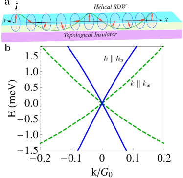
Figure 1: (Color online) (a) Schematic diagram of the system. The HSDW is on top of the topological insulator with the periodicity $L$. (b) Energy of charge carrier dispersion versus the wavevector $k$ with $k$ measured near the BZ center. Dashed (green) and solid (blue) lines show the dispersion along the $\hat{x}$ direction and along the $\hat{y}$ direction, respectively with $U_{0}=50$meV and $L=90$nm ($E(0,0)$ was shifted to zero).

While the above Bloch equation may be solved by numerical diagonalization to obtain numerical eigenvalues and eigenvectors, more insight can be obtained into the solutions around high symmetry points in the FBZ at $\bm{k}=0$ and at the BZB by using perturbation theory. The numerical results of diagonalizing Eq. 5 are shown in Fig. 2, Fig. 3 and Fig. 4. The total Hamiltonian $H_{0}+U$ of the TI+HSDW system is invariant under a composite symmetry $S=\Theta T$ where $\Theta$ is the time-reversal operator and $T$ is the operator corresponding to translation by $L/2$. Since, the operator $S$, similar to the time-reversal symmetry operator $\Theta$, is both anti-unitary and satisfies $S^{2}=-1$, the proximity to the HSDW does not open a gap at $\bm{k}=0$. In other words, the HSDW preserves the global time-reversal symmetry, it does not open up a gap near $\bm{k}=0$ on the TI surface.

In the limit of a perturbatively weak coupling to the HSDW ($\frac{|U({\bf G})|}{\hbar v_{F}|{\bf G}|}\ll 1$), the leading order contribution of the HSDW to the low-momentum $(\bm{k}\sim 0)$ dispersion can be characterized by the renormalization of the group velocity and effective mass at $\bm{k}=0$. The group velocity of states without the HSDW is isotropic around ${\bf k}=0$ with constant magnitude $v_{F}$. In presence of the HSDW, the renormalized group velocity of quasiparticles parallel to the wavevector ${\bf k}$ [$v_{\hat{k}}\equiv{\bf v}({\bf k})\cdot\hat{k}$] around the Dirac point ($|k|\ll 1$) obtained within second order perturbation theory can be written as

$$\begin{array}[]{l l l l l l }\dfrac{v_{\hat{k}}-v_{F}}{v_{F}}=\dfrac{1}{\hbar v_{F}}\dfrac{\partial(E_{+,k}-\varepsilon_{+,k})}{\partial k}=-\dfrac{U_{0}^{2}L^{2}}{8\pi^{2}\hbar^{2}v_{F}^{2}}(3+\cos 2\theta_{{\bf k}})\end{array}$$ (6)

From Eq. (6), it is clear that the renormalized group velocity is anisotropic around the Dirac point and decays monotonically, both with the amplitude of periodic potential $U_{0}$, and with the spatial period $L$ of the potential. Fig. 2 shows the result from a full numerical calculation. We note that there is good agreement between the trends from Eq. (6) and the full calculation (shown in Fig. 2a) for weak potential strength.

The interaction with the HSDW introduces at $\bm{k}\sim 0$ a finite curvature along the $\hat{x}$-direction to the previously linear in $\bm{k}$ dispersion of the Dirac fermions. The effective mass tensor at ${\bf k}=0$ from the curvature of the energy band around the Dirac point is given by

$$\Big{(}\dfrac{m_{e}}{m^{*}}\Big{)}_{\alpha\beta}\ =\ \dfrac{m_{e}}{\hbar^{2}}\dfrac{\partial^{2}E({\bf k})}{\partial k_{\alpha}\partial k_{\beta}}\Big{|}_{{\bf k}=0}=\Bigg{\{}\begin{array}[]{l l}0,\ \ \alpha,\beta=y,\ \text{or}\ \alpha\neq\beta\\ \\ \dfrac{8U_{0}^{2}m_{e}}{\hbar^{3}v_{F}G_{0}^{3}},\ \ \alpha,\beta=x\end{array}$$ (7)

where $m_{e}$ is the bare electron mass and $G_{0}=\dfrac{2\pi}{L}$. From Eq. (7) the effective mass $m_{e}/m_{xx}^{*}$ grows as $U_{0}^{2}$, which describes the small $U_{0}$ behavior of the numerically determined effective mass shown in Fig. 2b.

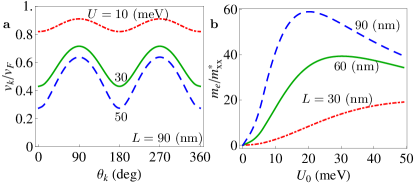
Figure 2: (Color online) (a) The group velocity $v_{\hat{k}}$ (measured from the Dirac point) of charge carriers on the surface of the TI in units of the Fermi velocity ($v_{F}$) versus the angle $\theta_{\bf k}$ with $L=90$nm. Dotdashed red, solid green and dashed blue lines correspond to $U_{0}$ being 10 meV, 30 meV and 50 meV, respectively. (b) The inverse effective mass $m_{e}/m_{xx}^{*}$ versus $U_{0}$ for the first band above the Dirac point on BZ center. Dotdashed red, solid green and dashed blue lines are results for $L$ being $30$nm, $60$nm and $90$nm, respectively.

II.2 Dirac Cone near BZ boundary

While the periodic potential from the HSDW introduces renormalizations of the velocity and effective masses at the center of the Dirac cone at $\bm{k}=0$, the effect of the periodic potential is limited to being perturbative since there is no degeneracy in the initial Dirac spectrum near $\bm{k}=0$. However, such degeneracies do occur at the edges of the FBZ, which we have referred to as the BZB, and non-perturbative effects of the potential may be generated by coherent back scattering with momenta $\bm{G}$. Unlike the case of conventional crystals, where such back-scattering opens up gaps, one finds the emergence of new Dirac cones at the BZB in the presence of interaction with the HSDW (Fig. 3a).

When the wavevector ${\bf k}$ is on the first BZB ($(k_{x},k_{y})=(\pi/L,k_{y})$), the two states $\left|s,{\bf k}\right>$ and $\left|s,{\bf k}-(2\pi/L,0)\right>$ are degenerate before the periodic potential is applied. In the presence of an applied potential, the largest contribution to the energy eigenvalues at the edges of the BZ comes from these two degenerate states. For the clockwise helix, the backscattering amplitude leads to an energy gap on the BZB that is given by,

$$\Delta E(k_{y})=U_{0}\left(1-\frac{s}{\sqrt{1+(k_{y}L/\pi)^{2}}}\right),$$ (8)

where $s=\pm 1$ represents the positive or negative bands in the Dirac cone. In the lower band of the Dirac cone, i.e. $s=-1$, the above gap is maximum at $k_{y}=0$ and decreases monotonically with $|k_{y}|$. The positive band is more interesting with a gap that vanishes at $k_{y}=0$. From the full numerical calculation in Fig. 3b, we can see that the energy gap of the positive band on the BZB increases monotonically then decreases with $k_{y}$.

If we change the sign of both $U_{y}$ and $U_{z}$, the physics will not change since the total Hamiltonian is invariant under this transformation $T$, where $T$ is the operator corresponding to translation by $L/2$ in the $\hat{x}$ direction. The chirality of the helix depends on the relative sign of the $U_{y}$ and $U_{z}$ in the HSDW potential. The effects of the clockwise helix on the upper band of the Dirac cone is the same as the anticlockwise helix on the lower band of the Dirac cone. For the anticlockwise helix, the minus sign in Eq. 8 should be changed to a plus sign, which leads to a vanishing gap at $k_{y}=0$ for the lower band.

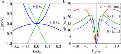
Figure 3: (Color online) (a) Semi-Dirac charge carrier dispersion versus the wavevector $k$ with $k$ measured from $(k_{x},k_{y})=(\dfrac{\pi}{L},0)$ on the BZB. Dashed (green) and solid (blue) lines show the linear dispersion along the $\hat{x}$ direction and the quadratic dispersion along the $\hat{y}$ direction, respectively with $U_{0}=50$meV, $L=90$nm and $G_{0}=2\pi/90$nm^-1 ($E(\pi/L,0)$ was shifted to zero). (b).The energy gap $\Delta E$ between the first and the second band at the BZB versus $k_{y}$ for charge carriers above the Dirac point with $U_{0}=50$meV and $G_{0}=2\pi/90$nm^-1. Dotdashed (red) , solid(green) and dashed (blue) lines correspond to $L$ being 30 nm, 60 nm and 90 nm, respectively.

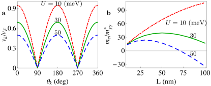
Figure 4: (Color online)  (a) Anisotropic $v_{\hat{k}}/v_{F}$ measured from the semi-Dirac point on the BZB versus the angle $\theta_{\bf k}$ with $L=90$nm. Dotdashed (red), solid (green) and dashed (blue) lines correspond to $U_{0}$ being 10 meV, 30 meV and 50 meV, respectively. (b) The inverse effective mass $m_{e}/m_{yy}^{*}$ versus $L$ around the point $(k_{x},k_{y})=(\dfrac{\pi}{L},0)$ for the lower band of the semi-Dirac point for three $U_{0}$. Note the negative effective mass (corresponding to Fig. 3 (a)).

As with the Dirac cone at $\bm{k}=0$, an understanding of the low-energy dispersion and the corresponding transport properties associated with the Dirac cone at the BZB is obtained by calculating the group velocity and effective mass. Second order perturbation theory leads to a strongly anisotropic group-velocity $v_{\hat{k}}$ measured from the gap-less point at $(k_{x},k_{y})=(\dfrac{\pi}{L},0)$ which is written as

$$v_{\hat{k}}=\dfrac{\hbar v_{F}^{2}G_{0}\cos\theta_{\bf k}}{\sqrt{U_{0}^{2}+\hbar^{2}v_{F}^{2}G_{0}^{2}}}$$ (9)

For comparison, the full numerical calculation is shown in Fig.4. The effective mass tensor at the new gapless point for the clockwise helix, calculated within second order perturbation theory similar to Eq. 7, is given by

$$\Big{(}\dfrac{m_{e}}{m^{*}}\Big{)}_{\alpha\beta}\Big{|}_{{\bf k}=(\pi/L,0)}=\Bigg{\{}\begin{array}[]{l l}0,\ \ \ \ \ \alpha,\beta=x,\ \text{or}\ \alpha\neq\beta\\ \\ 2(\hbar v_{F}G_{0}\pm U_{0})/G_{0}^{2},\ \ \ \alpha,\beta=y\end{array}$$ (10)

where the $\pm$ corresponds to the upper or lower band around the semi-Dirac point at $(k_{x},k_{y})=(\dfrac{\pi}{L},0)$. Eq. 9 and 10 together show the highly anisotropic dispersion of the semi-Dirac point on BZB: a dispersion linear along the periodic direction $\hat{x}$ but quadratic along the perpendicular direction $\hat{y}$. For the anticlockwise helix, the effective mass tensor given in Eq. 10 is still valid except now the gap for the lower band vanishes at $k_{y}=0$. Fig. 4a shows the angular dependence of the group velocity $v_{{\bf k}}$ from a full numerical calculation. The velocity $v_{y}$ is seen to have zero component regardless of the strength of the applied potential. The dependence of the renormalized group velocity $v_{k}/v_{F}$ is a decreasing function of the amplitude of the applied potential. In Fig. 4b, we plot the dependence of the inverse effective mass of the lower-band of the semi-Dirac point at the BZB (in the vicinity of $(k_{x},k_{y})=(\dfrac{\pi}{L},0)$) on the applied potential period $L$ and amplitude $U_{0}$ respectively. We find that the effective mass along the $\hat{y}$-direction changes sign from positive to negative as a function of $L$ and $U_{0}$. The dispersion at small $k_{y}$ for parameters $U,L_{0}$ corresponding to negative effective mass is shown in Fig. 3(a). In this case, the bands at larger $k_{y}$ turn up leading to the emergence of another fermi surface. There is no such fermi surface doubling for parameters with positive mass.

III Other forms of spin density wave

III.1 The HSDW with $U_{z}\neq U_{y}$

In this subsection, we shall discuss the case of a HSDW with different amplitudes in the $\hat{y}$ and $\hat{z}$ directions (i.e. $U_{y}\neq U_{z}$) with the propagation direction of the spin density wave still along the $\hat{x}$ direction. In order to study the effects of helical spin density wave with $U_{z}\neq U_{y}$, we first use the perturbation theory to calculate the renormalized velocity in the BZ center. In the limit of a perturbatively weak coupling to the HSDW ($\frac{|U({\bf G})|}{\hbar v_{F}|{\bf G}|}\ll 1$), the renormalization of group velocity (near the Dirac cone) given in Eq. 6 within second order perturbation theory should be modified to:

$$\begin{array}[]{l l l l l l }\dfrac{v_{\hat{k}}-v_{F}}{v_{F}}=-\dfrac{L^{2}}{8\pi^{2}\hbar^{2}v_{F}^{2}}\big{[}2U_{y}^{2}+U_{z}^{2}(1+\cos 2\theta_{{\bf k}})\big{]}\end{array}$$ (11)

It is clear that the above formula goes to Eq. 6 for the proper HSDW. We notice that the spin density wave in the $\hat{y}$ direction does not induce the anisotropic group velocity near the Dirac cone, which is also confirmed by the full numerical calculation. We present the angular dependence of the renormalized group velocity for two extreme limits $U_{y}=0$ and $U_{z}=0$ in Fig. 5.

We shall next explain the conditions for the appearance of the Dirac cones on the BZ boundary, which are supported by full numerical calculations as presented in Fig. 6 and 7. The largest contribution to the energy eigenvalues at the BZ boundary comes from these two degenerate states $\left|s,{\bf k}\right>$ and $\left|s,{\bf k}-(2\pi/L,0)\right>$, which are degenerate before applying the periodic potential. Only considering the above two states and using the relation $\theta_{{\bf k}-(2\pi/L,0)}=\pi-\theta_{{\bf k}}$ on the BZB, we can write down the two band Hamiltonian within perturbation theory as:

$$H({\bf k})=\left(\begin{array}[]{cc}s\hbar v_{F}\sqrt{\big{(}\dfrac{\pi}{L}\big{)}^{2}+k_{y}^{2}}&\frac{1}{2}(sU_{y}-U_{z}\cos\theta_{\bf k})(i\cos\theta_{\bf k}+\sin\theta_{\bf k})\\ \frac{1}{2}(sU_{y}-U_{z}\cos\theta_{\bf k})(-i\cos\theta_{\bf k}+\sin\theta_{\bf k})&s\hbar v_{F}\sqrt{\big{(}\dfrac{\pi}{L}\big{)}^{2}+k_{y}^{2}}\end{array}\right)\ ,$$ (12)

where $s=\pm 1$ denote the band index and $\theta_{\bf k}$ is the angle between the vector ${\bf k}$ and the $\hat{x}$ direction. Diagonalizing the above Hamiltonian we could get two eigenvalues written as:

$$\begin{array}[]{l l l l l }\epsilon_{1}=s\hbar v_{F}\sqrt{\big{(}\dfrac{\pi}{L}\big{)}^{2}+k_{y}^{2}}-\dfrac{1}{2}\sqrt{(sU_{y}-U_{z}\cos\theta_{\bf k})^{2}}\\ \\ \epsilon_{2}=s\hbar v_{F}\sqrt{\big{(}\dfrac{\pi}{L}\big{)}^{2}+k_{y}^{2}}+\dfrac{1}{2}\sqrt{(sU_{y}-U_{z}\cos\theta_{\bf k})^{2}}\\ \\ \Delta E=\mid sU_{y}-U_{z}\cos\theta_{\bf k}\mid,\end{array}$$ (13)

From the last equation in Eq. 13, we can clearly see that there are gapless states when $sU_{y}=U_{z}\cos\theta_{\bf k}$, since $0<\cos\theta_{\bf k}\leq 1$ for ${\bf k}$ on the BZ boundary (i.e. ${\bf k}=(\pi/L,k_{y})$). Therefore, we can have gapless states only for $U_{z}\geq U_{y}$. In addition, the energy charge carrier dispersion becomes parabolic along both $\hat{x}$ and $\hat{y}$ directions, which can be seen from Fig. 6(a) and 7(a). For the clockwise helix, the energy gap opened on the BZ boundary near ${\bf k}=(\pi/L,0)$ is shown as a function of $k_{y}$ for three different values of $U_{z,y}$. In Fig. 6(b) and Fig. 7(b) the energy gap is plotted as a function of $k_{y}$ for $U_{y}/U_{z}=0.8$ and $U_{z}/U_{y}=0.8$ respectively. It is seen that the energy gap is non-monotonic function of $|k_{y}|$ in the former, and monotonic in the latter case. The helical spin density with $U_{y}\neq U_{z}$ affect the energy charge carrier dispersion on the BZ center similar to the proper HSDW, rendering the Dirac cone on the BZ center highly anisotropic. The velocity of the Dirac cone along $\hat{x}$ direction (the helix propagates along the $\hat{x}$ direction) is smaller than that perpendicular to $\hat{x}$. When we go to the extreme limit , where one of the components $U_{y,z}$ is set to zero (the spin density wave), the energy gap in the presence of the spin density wave with magnetization in only one direction ($\hat{y}$ or $\hat{z}$), further simplifies to:

$$\Delta E=\Bigg{\{}\begin{array}[]{l l l l l }\mid U_{z}\cos\theta_{\bf k}\mid,\ \ \ \ U_{y}=0\\ \\ \mid U_{y}\mid,\ \ \ \ \ \ \ \ \ \ \ \ U_{z}=0\end{array}$$ (14)

Full numerical calculation shows (see Fig 8) the dependence on $k_{y}$ for the energy gap opened on the BZB with the presence of the spin density waves in either $\hat{z}$ or $\hat{y}$ direction. The latter dependence is not predicted correctly within the second order perturbation theory which suggests that the energy gap for $U_{z}=0$ is independent of $k_{y}$ (see second line of Eq. 14). Finally, one should note that the Hamiltonian has different symmetries along $\hat{y}$ and $\hat{z}$ directions. For a spin density wave only in the $\hat{y}$ direction, the total Hamiltonian satisfies the relation: $\sigma_{z}H\sigma_{z}=-H$, from which we can see that the upper and the lower band of the Dirac cone are symmetric. While for the spin density wave only in the $\hat{z}$ direction, the total Hamiltonian satisfies particle-hole symmetry, i.e. $\sigma_{x}H^{*}(-{\bf k})\sigma_{x}=-H({\bf k})$. The upper and the lower band of the Dirac cone are also symmetric when the spin density wave only has component in $\hat{z}$ direction. The velocity perpendicular to the $\hat{x}$, which is the same as the original Fermi velocity of $Bi_{2}Se_{3}$, remains unaffected in the presence of the periodic potential in the $\hat{z}$ direction.

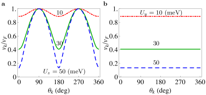
Figure 5: (Color online) (a) The group velocity $v_{\hat{k}}$ (measured from the Dirac point) of charge carriers on the surface of the TI in units of the Fermi velocity ($v_{F}$) versus the angle $\theta_{\bf k}$ with $L=90$nm and $U_{y}=0$. Dotdashed red, solid green and dashed blue lines correspond to $U_{z}$ being 10 meV, 30 meV and 50 meV, respectively. (b) The group velocity $v_{\hat{k}}$ (measured from the Dirac point) of charge carriers on the surface of the TI in units of the Fermi velocity ($v_{F}$) versus the angle $\theta_{\bf k}$ with $L=90$nm and $U_{z}=0$. Dotdashed red, solid green and dashed blue lines correspond to $U_{y}$ being 10 meV, 30 meV and 50 meV, respectively.

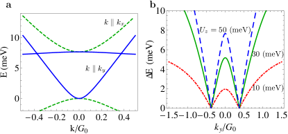
Figure 6: (Color online)  (a) Energy charge carrier dispersion versus the wavevector $k$ with $k$ measured from $(k_{x},k_{y})=(\dfrac{\pi}{L},0)$ on the BZB. Dashed (green) and solid (blue) lines show the linear dispersion along the $\hat{x}$ direction and the quadratic dispersion along the $\hat{y}$ direction, respectively with $U_{z}=50$meV, $U_{y}=40$meV, $L=90$nm and $G_{0}=2\pi/90$nm^-1 ($E(\pi/L,0)$ was shifted to zero). (b)The energy gap $\Delta E$ between the first and the second band at the BZB versus $k_{y}$ for charge carriers above the Dirac point with $L=90$nm and $U_{y}=0.8U_{z}$. Dotdashed (red) , solid(green) and dashed (blue) lines correspond to $U_{z}$ being 10 meV, 30 meV and 50 meV, respectively.

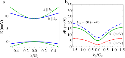
Figure 7: (Color online)  (a) Energy charge carrier dispersion versus the wavevector $k$ with $k$ measured from $(k_{x},k_{y})=(\dfrac{\pi}{L},0)$ on the BZB. Dashed (green) and solid (blue) lines show the linear dispersion along the $\hat{x}$ direction and the quadratic dispersion along the $\hat{y}$ direction, respectively with $U_{z}=40$meV, $U_{y}=50$meV, $L=90$nm and $G_{0}=2\pi/90$nm^-1 ($E(\pi/L,0)$ was shifted to zero). (b)The energy gap $\Delta E$ between the first and the second band at the BZB versus $k_{y}$ for charge carriers above the Dirac point with $L=90$nm and $U_{z}=0.8U_{y}$. Dotdashed (red) , solid(green) and dashed (blue) lines correspond to $U_{y}$ being 10 meV, 30 meV and 50 meV, respectively.

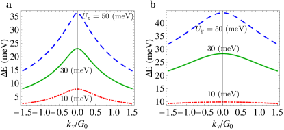
Figure 8: (Color online)  (a) The energy gap $\Delta E$ between the first and the second band at the BZB versus $k_{y}$ for charge carriers above the Dirac point with $L=90$nm and $U_{y}=0$. Dotdashed (red) , solid(green) and dashed (blue) lines correspond to $U_{z}$ being 10 meV, 30 meV and 50 meV, respectively. (b)The energy gap $\Delta E$ between the first and the second band at the BZB versus $k_{y}$ for charge carriers above the Dirac point with $L=90$nm and $U_{z}=0$. Dotdashed (red) , solid(green) and dashed (blue) lines correspond to $U_{y}$ being 10 meV, 30 meV and 50 meV, respectively.

III.2 Cycloidal spin density wave

In this subsection, we analyze the effects of the cycloidal spin density wave on the surface states of topological insulator. In the presence of the cycloidal spin density wave on top of the topological insulatorRö$\beta$ler et al. (2010); Przeniosło et al. (2006), the potential is modified to:

$$\begin{array}[]{l l }U_{c}(x)=U_{x}\sigma_{x}\cos(\dfrac{2\pi}{L}x)+U_{y,z}\sigma_{y,z}\sin(\dfrac{2\pi}{L}x),\end{array}$$ (15)

The term involving $\sigma_{x}$ in the magnetic potential will disappear under the gauge transformation:

$$\begin{array}[]{l l }e^{-iA(x)}He^{iA(x)}=H_{0}+U_{y,z}\sigma_{y,z}\sin(\dfrac{2\pi}{L}x),\end{array}$$ (16)

where $H_{0}$ is the single Dirac fermion Hamiltonian without applied potential as given in Eq. 1 and the function $A(x)$ is given by:

$$A(x)=-\dfrac{U_{x}L}{2\pi\hbar}\sin\big{(}\dfrac{2\pi x}{L}\big{)}$$ (17)

For the general periodic function of spin density wave along $\hat{x}$ direction, i.e. $F(x)\sigma_{x}$, the $\sigma_{x}$ term will disappear if we apply the gauge transformation $e^{iA_{F}(x)}$ with $A_{F}(x)=-\int^{x}_{c}F(x^{\prime})/\hbar dx^{\prime}$ ($c$ is any constant). Thus, the effects of the cycloidal spin density wave comes from the term with $\sigma_{y,z}$, which goes to the extreme limit as discussed in Sec.III.1.

IV Summary and Conclusions

In summary, we have considered the effects of a helical spin density wave on the surface states of a topological insulator and also the effects of other spin density wave on the surface transport property of topological insulator. We find that the HSDW acts like an effective spin potential on the TI surface and breaks the local time reversal invariance in the latter. The applied spin potential has two main consequences: First, the group velocity of electrons at the Dirac point is strongly suppressed in the direction transverse to the periodic potential. Secondly, new semi-Dirac points emerge for the first upper (lower) band at the Brillouin zone boundaries that corresponds to the right-handed (left-handed) chirality of the applied proper HSDW. The semi-Dirac points are characterized by linear dispersion parallel to the direction $\hat{x}$ of the applied periodic potential but quadratic dispersion perpendicular to the $\hat{x}$ direction. When the chemical potential of the TI is such that the semi-Dirac points at the BZBs give the main contribution to transport, we expect the surface transport properties to be highly anisotropic. This is because at these points, the dispersion is linear in one direction and quadratic in the other. The momentum space location of these new semi-Dirac cones can also be manipulated by applying an in-plane magnetic field to the HSDW. Such a magnetic field Cheong and Mostovoy (2007) can change the orientation of the spin rotation axis relative to the pitch vector of the HSDW. By studying the effects of such a change in the applied periodic potential on the new semi-Dirac cones and measuring the anisotropic component of the transport, it should be possible to isolate the surface state contribution from the bulk in the total conductance in topological insulators with relatively small bulk gaps. The number of Dirac cones appearing on the BZ boundary is determined by the relative ratio of $U_{z}/U_{y}$, which could be zero, one or two corresponding to $U_{z}/U_{y}<1$, $U_{z}/U_{y}=1$ and $U_{z}/U_{y}>1$, respectively. We also prove that the spin density wave with spin vectors along $\hat{x}$ direction will not change the surface transport property of a three dimensional topological insulator. One particular advantage of our proposal is that the proposed experiment can be carried out in the existing TI systems without any problem arising from the bulk conduction (as a result of unintentional bulk doping by defects), which is invariably present in almost all current TI systems, since the bulk transport is isotropic and presumably unaffected by the presence of the HSDW.

Although the proposed system in this work is a sandwich structure of a TI and a multiferroic, we believe that this structure may turn out to be a suitable candidate for the direct manifestation of the elusive 2D transport properties even in the presence of considerable bulk conduction since the anisotropy introduced by the presence of the HSDW would only affect the surface transport properties without affecting much the bulk conduction behavior. Given the great current interest and activity in the observation of the 2D surface transport properties in TI materials Ren et al. (2010); Qu et al. (2010); Butch et al. (2010); Analytis et al. (2010); Culcer et al. (2010); Checkelsky et al. ; Taskin et al. (2010); Nishide et al. (2010); Eto et al. (2010); Sarma et al. , we are optimistic that our proposed structure could go a long way in establishing the experimental behavior of 2D surface transport in topological insulators.