Abstract

The present study deals with a spatially homogeneous and anisotropic Bianchi-II cosmological model representing massive strings. The energy-momentum tensor, as formulated by Letelier (1983), has been used to construct a massive string cosmological model for which the expansion scalar is proportional to one of the components of shear tensor. The Einstein’s field equations have been solved by applying a variation law for generalized Hubble’s parameter that yields a constant value of deceleration parameter in Bianchi-II space-time. A comparative study of accelerating and decelerating modes of the evolution of universe has been carried out in the presence of string scenario. The study reveals that massive strings dominate the early Universe. The strings eventually disappear from the Universe for sufficiently large times, which is in agreement with the current astronomical observations.

Keywords: Massive string, Bianchi-II model, Accelerating universe

PACS number: 98.80.Cq, 04.20.-q, 04.20.Jb

1 Introduction

In recent years, there has been considerable interest in string cosmology. Cosmic strings are topologically stable objects which might be found during a phase transition in the early universe (Kibble [1]). Cosmic strings play an important role in the study of the early Universe. These arise during the phase transition after the big bang explosion as the temperature goes down below some critical temperature as predicted by grand unified theories (Zel’dovich et al. [2]; Kibble [1, 3]; Everett [4]; Vilenkin [5]). It is believed that cosmic strings give rise to density perturbations which lead to the formation of galaxies (Zel’dovich [6]). However, recent observations suggest that cosmic strings cannot be wholly responsible for either the CMB fluctuations or the observed clustering of galaxies [7, 8]. The cosmic strings have stress-energy, and couple to the gravitational field. Therefore, it is interesting to study the gravitational effects that arise from strings. The pioneering work in the formulation of the energy-momentum tensor for classical massive strings was done by Letelier [9] who considered the massive strings to be formed by geometric strings with particle attached along its extension. Letelier [10] first used this idea in obtaining cosmological solutions in Bianchi-I and Kantowski-Sachs space-times. Stachel [11] has studied massive string.

The present day Universe is satisfactorily described by homogeneous and isotropic models given by the FRW space-time. But at smaller scales, the Universe is neither homogeneous and isotropic nor do we expect the Universe in its early stages to have these properties. Homogeneous and anisotropic cosmological models have been widely studied in the framework of general relativity in the search of a realistic picture of the Universe in its early stages. Although these are more restricted than the inhomogeneous models which explain a number of observed phenomena quite satisfactorily. A spatially homogeneous Bianchi model necessarily has a three-dimensional group, which acts simply transitively on space-like three-dimensional orbits. Here we confine ourselves to models of Bianchi-II. Asseo and Sol [12] emphasized the importance of Bianchi type-II Universe. Bianchi type-II space-time has a fundamental role in constructing cosmological models suitable for describing the early stages of evolution of Universe.

Roy and Banerjee [13] have dealt with locally rotationally symmetric (LRS) cosmological models of Bianchi type-II representing clouds of geometrical as well as massive strings. Wang [14] studied the Letelier model in the context of LRS Bianchi type-II space-time. Recently, Pradhan et al. [15, 16] and Amirhashchi and Zainuddin [17] obtained LRS Bianchi type II cosmological models with perfect fluid distribution of matter and string dust, respectively. Belinchon [18, 19] studied Bianchi type-II space-time in connection with massive cosmic string and perfect fluid models with time varying constants under the self-similarity approach respectively. Recently, Tyagi and Sharma [20] have investigated string cosmological models in Bianchi type-II space-time.

Motivated by the above discussions, in this paper, we have investigated a new class of Bianchi type-II cosmological models for a cloud of strings by using the law of variation for generalized mean Hubble’s parameter. This approach is different from what the other authors have adapted. The paper is organized as follows. The metric and the field equations are presented in Section 2. Section 3 deals with exact solutions of the field equations with cloud of strings. Physical behavior of the derived model is elaborated in detail. Finally, in Section 4, concluding remarks are given.

2 The metric and field equations

We consider totally anisotropic Bianchi type-II line element, given by

$$ds^{2}=-dt^{2}+A^{2}(dx-zdy)^{2}+B^{2}dy^{2}+C^{2}dz^{2},$$ (1)

where the metric potentials $A$, $B$ and $C$ are functions of $t$ alone. This ensures that the model is spatially homogeneous.

The Einstein’s field equations ( in gravitational units $c=1,8\pi G=1$) read as

$$G^{i}_{j}=-T^{i}_{j},$$ (2)

where $G^{i}_{j}=R^{i}_{j}-\frac{1}{2}Rg^{i}_{j}$ is the Einstein tensor. The energy-momentum tensor $T^{i}_{j}$ for a cloud of massive strings and perfect fluid distribution is taken as

$$T^{i}_{j}=(\rho+p)v^{i}v_{j}+pg^{i}_{j}-\lambda x^{i}x_{j},$$ (3)

where $p$ is the isotropic pressure; $\rho$ is the proper energy density for a cloud strings with particles attached to them; $\lambda$ is the string tension density; $v^{i}=(0,0,0,1)$ is the four-velocity of the particles, and $x^{i}$ is a unit space-like vector representing the direction of string. The vectors $v^{i}$ and $x^{i}$ satisfy the conditions

$$v_{i}v^{i}=-x_{i}x^{i}=-1,\;\;v^{i}x_{i}=0.$$ (4)

Choosing $x^{i}$ parallel to $\partial/\partial z$, we have

$$x^{i}=(0,0,C^{-1},0).$$ (5)

Here the cosmic string has been directed along z-direction in order to satisfy the condition $T^{1}_{1}=T^{2}_{2}$. As a result, the off-diagonal component of Einstein tensor, viz., $G^{1}_{2}=z(T^{2}_{2}-T^{1}_{1})$ vanishes. A detailed analysis about the choice of energy-momentum tensor for Bianchi type-II models is given by Saha [21].

If the particle density of the configuration is denoted by $\rho_{p}$, then

$$\rho=\rho_{p}+\lambda.$$ (6)

The Einstein’s field equations (2) for line element (1) with energy-momentum tensor (3), lead to the following set of independent differential equations:

$$\frac{\ddot{B}}{B}+\frac{\ddot{C}}{C}+\frac{\dot{B}\dot{C}}{BC}-\frac{3}{4}\frac{A^{2}}{B^{2}C^{2}}=-p\;,$$ (7)

$$\frac{\ddot{C}}{C}+\frac{\ddot{A}}{A}+\frac{\dot{C}\dot{A}}{CA}+\frac{1}{4}\frac{A^{2}}{B^{2}C^{2}}=-p\;,$$ (8)

$$\frac{\ddot{A}}{A}+\frac{\ddot{B}}{B}+\frac{\dot{A}\dot{B}}{AB}+\frac{1}{4}\frac{A^{2}}{B^{2}C^{2}}=-p+\lambda\;,$$ (9)

$$\frac{\dot{A}\dot{B}}{AB}+\frac{\dot{B}\dot{C}}{BC}+\frac{\dot{C}\dot{A}}{CA}-\frac{1}{4}\frac{A^{2}}{B^{2}C^{2}}=\rho\;.$$ (10)

Here, and in what follows, an over dot indicates ordinary differentiation with respect to $t$. The energy conservation equation $\;T^{ij}_{\;\;\;;j}=0$, leads to the following expression:

$$\dot{\rho}+(\rho+p)\left(\frac{\dot{A}}{A}+\frac{\dot{B}}{B}+\frac{\dot{C}}{C}\right)-\lambda\frac{\dot{C}}{C}=0\;,$$ (11)

which is a consequence of the field equations (7)-(10).

3 Solutions of the Field Equations

Equations (7)-(10) are four equations in six unknown parameters $A$, $B$, $C$, $p$, $\rho$ and $\lambda$. Two additional constraints relating these parameters are required to obtain explicit solutions of the system.

First, we utilize the special law of variation for the Hubble’s parameter given by Berman [22], which yields a constant value of deceleration parameter. Here, the law reads as

$$H=\ell(ABC)^{-\frac{n}{3}},$$ (12)

where $\ell>0$ and $n\geq 0$ are constants. Such type of relations have already been considered by Berman and Gomide [23] for solving FRW models. Later on, many authors (see, Kumar and Singh [24], Akarsu and Kilinc [25] and references therein) have studied flat FRW and Bianchi type models by using the special law for Hubble’s parameter that yields constant value of deceleration parameter.

Considering $(ABC)^{\frac{1}{3}}$ as the average scale factor of the anisotropic Bianchi-II space-time, the average Hubble’s parameter may be written as

$$H=\frac{1}{3}\left(\frac{\dot{A}}{A}+\frac{\dot{B}}{B}+\frac{\dot{C}}{C}\right).$$ (13)

Equating the right hand sides of (12) and (13), and integrating, we obtain

$$ABC=(n\ell t+c_{1})^{\frac{3}{n}},\;\;\;\;(n\neq 0)$$ (14)

$$ABC=c_{2}^{3}e^{3\ell t},\;\;\;\;(n=0)$$ (15)

where $c_{1}$ and $c_{2}$ are constants of integration. Thus, the law (12) provides power-law (14) and exponential-law (15) of expansion of the Universe.

Following Pradhan and Chouhan [26], we assume that the component $\sigma^{1}_{~{}1}$ of the shear tensor $\sigma^{j}_{~{}i}$ is proportional to the expansion scalar ($\theta$). This condition leads to the following relation between the metric potentials:

$$A=(BC)^{m},$$ (16)

where $m$ is a positive constant.

Now, subtracting (8) from (7), and taking integral of the resulting equation two times, we get

$$\frac{B}{A}=c_{4}\exp\left[\int\left\{\frac{1}{ABC}\int\frac{A^{3}}{BC}dt\right\}dt+c_{3}\int\frac{1}{ABC}dt\right],$$ (17)

where $\;c_{3}$ and $\;c_{4}$ are constants of integration. In the following subsections, we discuss the string cosmology using the power-law (14) and exponential-law (15) of expansion of the Universe.

3.1 String Cosmology with Power-law

Solving the equations (14), (16) and (17), we obtain the metric functions as

$$A(t)=(n\ell t+c_{1})^{\frac{3m}{n(m+1)}}\;,$$ (18)

$$B(t)=c_{4}(n\ell t+c_{1})^{\frac{3m}{n(m+1)}}\exp{\left[\frac{(m+1)^{2}}{2\ell^{2}M}(n\ell t+c_{1})^{\frac{6(m-1)}{n(m+1)}+2}+\frac{c_{3}}{\ell(n-3)}(n\ell t+c_{1})^{\frac{n-3}{n}}\right]}\;,$$ (19)

$$C(t)=c_{4}^{-1}(n\ell t+c_{1})^{\frac{3(1-m)}{n(m+1)}}\exp{\left[-\frac{(m+1)^{2}}{2\ell^{2}M}(n\ell t+c_{1})^{\frac{6(m-1)}{n(m+1)}+2}-\frac{c_{3}}{\ell(n-3)}(n\ell t+c_{1})^{\frac{n-3}{n}}\right]}\;,$$ (20)

where $M=(9m-3+mn+n)(3m-3+mn+n)$ and $\;n\neq 3$.

In the special case $n=3$, we have

$$A(t)=(3\ell t+c_{1})^{\frac{m}{m+1}}\;,$$ (21)

$$B(t)=c_{4}(3\ell t+c_{1})^{\frac{3m\ell+c_{3}(m+1)}{3\ell(m+1)}}\exp{\left[\frac{(m+1)^{2}}{144\ell^{2}m^{2}}(3\ell t+c_{1})^{\frac{4m}{m+1}}\right]}\;,$$ (22)

$$C(t)=c_{4}^{-1}(3\ell t+c_{1})^{\frac{3(1-m)\ell-c_{3}(m+1)}{3\ell(m+1)}}\exp{\left[-\frac{(m+1)^{2}}{144\ell^{2}m^{2}}(3\ell t+c_{1})^{\frac{4m}{m+1}}\right]}\;,$$ (23)

Thus, the metric (1) is completely determined.

The expressions for the isotropic pressure ($p$), the proper energy density ($\rho$), the string tension ($\lambda$) and the particle density ($\rho_{p}$) for the above model are obtained as

$$p = \frac{3\ell^{2}[n(m+1)-3(m^{2}-m+1)]}{(m+1)^{2}}(n\ell t+c_{1})^{-2}+\frac{3(m+1)(n+1)}{4(9m-3+mn+n)}(n\ell t+c_{1})^{-\frac{6(1-m)}{n(m+1)}}$$ (24)

$$+\frac{3c_{3}\ell(1-2m)}{m+1}(n\ell t+c_{1})^{-\frac{3}{n}-1}-\frac{(m+1)^{2}}{\ell^{2}(9m-3+mn+n)^{2}}(n\ell t+c_{1})^{-\left[\frac{12(1-m)}{n(m+1)}-2\right]}$$

$$-\frac{2c_{3}(m+1)}{\ell(9m-3+mn+n)}(n\ell t+c_{1})^{-\left[\frac{3(3-m)}{n(m+1)}-1\right]}-c_{3}^{2}(n\ell t+c_{1})^{-\frac{6}{n}},$$

$$\rho = \frac{9\ell^{2}m(2-m)}{(m+1)^{2}}(n\ell t+c_{1})^{-2}+\frac{15-33m-mn-n}{4(9m-3+mn+n)}(n\ell t+c_{1})^{-\frac{6(1-m)}{n(m+1)}}$$ (25)

$$+\frac{3c_{3}\ell(1-2m)}{m+1}(n\ell t+c_{1})^{-\frac{3}{n}-1}-\frac{(m+1)^{2}}{\ell^{2}(9m-3+mn+n)^{2}}(n\ell t+c_{1})^{-\left[\frac{12(1-m)}{n(m+1)}-2\right]}$$

$$-\frac{2c_{3}(m+1)}{\ell(9m-3+mn+n)}(n\ell t+c_{1})^{-\left[\frac{3(3-m)}{n(m+1)}-1\right]}-c_{3}^{2}(n\ell t+c_{1})^{-\frac{6}{n}},$$

$$\lambda=\frac{3\ell^{2}(2m-1)(3-n)}{m+1}(n\ell t+c_{1})^{-2}+2(n\ell t+c_{1})^{-\frac{6(1-m)}{n(m+1)}}\;,$$ (26)

$$\rho_{p} = \frac{3\ell^{2}[3m(2-m))+(3-n)(1-2m)(m+1)]}{(m+1)^{2}}(n\ell t+c_{1})^{-2}+\frac{3(13-35m-3mn-3n)}{4(9m-3+mn+n)}(n\ell t+c_{1})^{-\frac{6(1-m)}{n(m+1)}}$$ (27)

$$+\frac{3c_{3}\ell(1-2m)}{m+1}(n\ell t+c_{1})^{-\frac{3}{n}-1}-\frac{(m+1)^{2}}{\ell^{2}(9m-3+mn+n)^{2}}(n\ell t+c_{1})^{-\left[\frac{12(1-m)}{n(m+1)}-2\right]}$$

$$-\frac{2c_{3}(m+1)}{\ell(9m-3+mn+n)}(n\ell t+c_{1})^{-\left[\frac{3(3-m)}{n(m+1)}-1\right]}-c_{3}^{2}(n\ell t+c_{1})^{-\frac{6}{n}}.$$

The above solutions satisfy the energy conservation equation (11) identically, as expected.

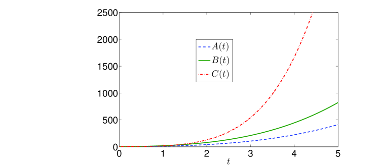
Figure 1: Scale factors vs time with $n=0.5$, $m=0.4$, $\ell=2$, $c_{1}=c_{3}=1$ and $c_{4}=2$.

We observe that all the parameters diverge at $t=-c_{1}/n\ell$. Therefore, the model has a singularity at $t=-c_{1}/n\ell$, which can be shifted to $t=0$ by choosing $c_{1}=0$. This singularity is of Point Type as all the scale factors vanish at $t=-c_{1}/n\ell$. The cosmological evolution of Bianchi-II space-time is expansionary since all the scale factors monotonically increase with time (see, Fig.1). So, the Universe starts expanding with a big bang singularity in the derived model. The parameters $p$, $\rho$, $\rho_{p}$ and $\lambda$ start off with extremely large values. In particular, the large values of $\rho_{p}$ and $\lambda$ in the beginning suggest that strings dominate the early Universe. For sufficiently large times, $\rho_{p}$ and $\lambda$ become negligible. Therefore, the strings disappear from the Universe for larger times. That is why, the strings are not observable in the present Universe.

The rates of expansion in the direction of $x$, $y$ and $z$ are given by

$$H_{x}=\frac{\dot{A}}{A}=\frac{3m\ell}{m+1}(n\ell t+c_{1})^{-1}\;,$$ (28)

$$H_{y}=\frac{\dot{B}}{B}=\frac{3m\ell}{m+1}(n\ell t+c_{1})^{-1}+\frac{m+1}{\ell(9m-3+mn+n)}(n\ell t+c_{1})^{-\frac{6(1-m)}{n(m+1)}+1}+c_{3}(n\ell t+c_{1})^{-\frac{3}{n}}\;,$$ (29)

$$H_{z}=\frac{\dot{C}}{C}=\frac{3(1-m)\ell}{m+1}(n\ell t+c_{1})^{-1}-\frac{m+1}{\ell(9m-3+mn+n)}(n\ell t+c_{1})^{-\frac{6(1-m)}{n(m+1)}+1}-c_{3}(n\ell t+c_{1})^{-\frac{3}{n}}.$$ (30)

The average Hubble’s parameter, expansion scalar and shear of the model are, respectively given by

$$H=\frac{1}{3}(H_{x}+H_{y}+H_{z})=\ell(n\ell t+c_{1})^{-1},$$ (31)

$$\theta=3H=3\ell(n\ell t+c_{1})^{-1},$$ (32)

$$\sigma^{2} = \frac{1}{6}\left[(H_{x}-H_{y})^{2}+(H_{y}-H_{z})^{2}+(H_{z}-H_{x})^{2}\right]$$ (33)

$$= \frac{3\ell^{2}(2m-1)^{2}}{(m+1)^{2}}(n\ell t+c_{1})^{-2}-\frac{15-33m-mn-n}{4(9m-3+mn+n)}(n\ell t+c_{1})^{-\frac{6(1-m)}{n(m+1)}}$$

$$-\frac{3c_{3}\ell(1-2m)}{m+1}(n\ell t+c_{1})^{-\frac{3}{n}-1}+\frac{(m+1)^{2}}{\ell^{2}(9m-3+mn+n)^{2}}(n\ell t+c_{1})^{-\left[\frac{12(1-m)}{n(m+1)}-2\right]}$$

$$+\frac{2c_{3}(m+1)}{\ell(9m-3+mn+n)}(n\ell t+c_{1})^{-\left[\frac{3(3-m)}{n(m+1)}-1\right]}+c_{3}^{2}(n\ell t+c_{1})^{-\frac{6}{n}}.$$

The spatial volume ($V$) and anisotropy parameter $(\bar{A})$ are found to be

$$V=ABC=(n\ell t+c_{1})^{\frac{3}{n}},$$ (34)

$$\bar{A} = \frac{2\sigma^{2}}{3H^{2}}=\frac{2(2m-1)^{2}}{(m+1)^{2}}-\frac{15-33m-mn-n}{6\ell^{2}(9m-3+mn+n)}(n\ell t+c_{1})^{-\frac{6(1-m)}{n(m+1)}+2}$$ (35)

$$-\frac{2c_{3}(1-2m)}{\ell(m+1)}(n\ell t+c_{1})^{-\frac{3}{n}+1}+\frac{2(m+1)^{2}}{3\ell^{4}(9m-3+mn+n)^{2}}(n\ell t+c_{1})^{-\left[\frac{12(1-m)}{n(m+1)}-4\right]}$$

$$+\frac{4c_{3}(m+1)}{3\ell^{3}(9m-3+mn+n)}(n\ell t+c_{1})^{-\left[\frac{3(3-m)}{n(m+1)}-3\right]}+\frac{2c_{3}^{2}}{3\ell^{2}}(n\ell t+c_{1})^{-\frac{6}{n}+2}.$$

The value of DP ($q$) is found to be

$$q=-1+\frac{\dot{H}}{H^{2}}=n-1,$$ (36)

which is a constant. A positive sign of $q$, i.e., $n>1$ corresponds to the standard decelerating model whereas the negative sign of $q$, i.e., $0<n<1$ indicates acceleration. The expansion of the Universe at a constant rate corresponds to $n=1$, i.e., $q=0$. Also, recent observations of SN Ia [27]-[34] reveal that the present Universe is accelerating and value of DP lies somewhere in the range $-1<q<0.$ It follows that in the derived model, one can choose the values of DP consistent with the observations.

From the above results, it can be seen that the spatial volume is zero at $t=-c_{1}/n\ell$, and it increases with the cosmic time $t$. The parameters $H_{x}$, $H_{y}$, $H_{z}$, $H$, $\theta$ and $\sigma$ diverge at the initial singularity. These parameters decrease with the evolution of Universe, and finally drop to zero at late times provided $m<1$. The mean anisotropy parameter asymptotically approaches to $\frac{2(2m-1)^{2}}{(m+1)^{2}}$ for $n<3$ and $m<1$. Thus, the dynamics of the mean anisotropy parameter depends on the values of $n$ and $m$. The model does not approach isotropy provided $m\neq 0.5$ as may be observed from Fig. 1. In case $m=0.5$, at late times, the directional scale factors vary as

$$A(t)\approx(n\ell t+c_{1})^{\frac{1}{n}},\;\;B(t)\approx(n\ell t+c_{1})^{\frac{1}{n}},\;\;C(t)\approx(n\ell t+c_{1})^{\frac{1}{n}}.$$

Therefore, isotropy is achieved in the derived model for $m=0.5$. Since the present-day Universe is isotropic, we consider $m=0.5$ in the remaining discussion of the model.

For $n<1$, the model is accelerating whereas for $n>1$ it goes to decelerating phase. In what follows, we compare the two modes of evolution through graphical analysis of various parameters. We have chosen $n=2$, i.e., $q=1$ to describe the decelerating phase while the accelerating mode has been accounted by choosing $n=0.5$, i.e., $q=-0.5$. The other constants are chosen as $\ell=6$, $c_{1}=1$, $c_{3}=1$, $m=0.5$.

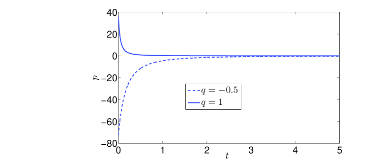
Figure 2: Pressure vs time.

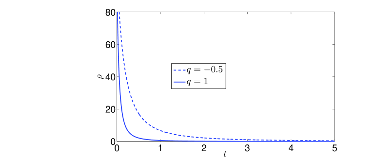
Figure 3: Rest energy density vs time.

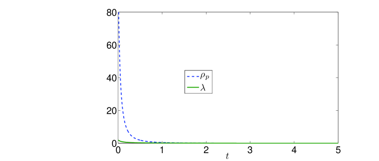
Figure 4: Particle energy density and string tension vs time for $q=1$.

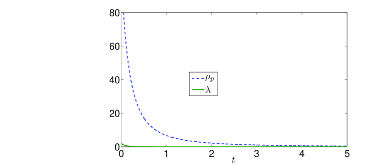
Figure 5: Particle energy density and string tension vs time for $q=-0.5$.

Fig. 2 depicts the variation of pressure versus time in the two modes of evolution of the Universe. We observe that the pressure is positive in the decelerating Universe which decreases with the evolution of the Universe. But in the accelerating phase, negative pressure dominates the Universe, as expected. In both cases, the pressure becomes negligible at late times.

The rest energy density has been graphed versus time in Fig. 3. It is evident that the rest energy density remains positive in both modes of evolution. However, it decreases more sharply with the cosmic time in the decelerating Universe.

Fig. 4 and Fig. 5 show the behavior of particle energy density and string tension versus time in the decelerating and accelerating modes, respectively. We see that $\rho_{p}>\lambda$, i.e., the particle energy density remains larger than the string tension density during the cosmic expansion , especially in early Universe. This shows that massive strings dominate the early Universe (see, Refs. [1, 19]). Further, it is observed that for sufficiently large times, $\rho_{p}$ and $\lambda$ tend to zero. Therefore, the strings disappear from the Universe at late times.

According to Ref. [19], since there is no direct evidence of strings in the present-day Universe, we are in general, interested in constructing models of a Universe that evolves purely from the era dominated by either geometric string or massive strings and ends up in a particle dominated era with or without remnants of strings. Therefore, the above model describes the evolution of the Universe consistent with the present-day observations.

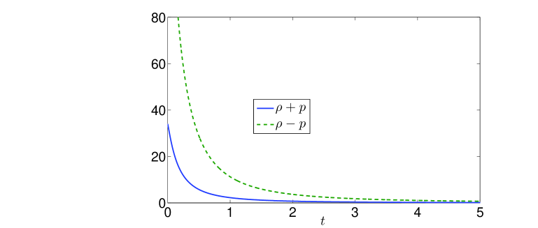
Figure 6: $\rho+p$ and $\rho-p$ vs time for $q=-0.5$.

From Fig. 3 to Fig. 6, we observe the following:

(i) $\rho\geq 0$

(ii) $\rho_{p}\geq 0$

(iii) $\rho+p\geq 0$

(iv) $\rho-p\geq 0$.

This shows that the weak and dominant energy conditions are satisfied in the derived model.

3.2 String Cosmology with Exponential-law

Solving the equations (15), (16) and (17), we obtain the metric functions as

$$A(t)=c_{2}^{\frac{3m}{m+1}}\exp{\left(\frac{3m\ell}{m+1}t\right)}\;,$$ (37)

$$B(t)=c_{4}c_{2}^{\frac{3m}{m+1}}\exp{\left[\frac{3m\ell}{m+1}t+\frac{c_{2}^{\frac{6(m-1)}{m+1}}(m+1)^{2}}{18\ell^{2}(3m-1)(m-1)}e^{\frac{6\ell(m-1)}{m+1}t}-\frac{c_{3}}{3\ell c_{2}^{3}}e^{-3\ell t}\right]},$$ (38)

$$C(t)=c_{4}^{-1}c_{2}^{\frac{3(1-m)}{m+1}}\exp{\left[\frac{3(1-m)\ell}{m+1}t-\frac{c_{2}^{\frac{6(m-1)}{m+1}}(m+1)^{2}}{18\ell^{2}(3m-1)(m-1)}e^{\frac{6\ell(m-1)}{m+1}t}+\frac{c_{3}}{3\ell c_{2}^{3}}e^{-3\ell t}\right]}.$$ (39)

The expressions for the isotropic pressure, the proper energy density, the string tension and the particle density for the derived model are obtained as

$$p = -\frac{9\ell^{2}(m^{2}-m+1)}{(m+1)^{2}}+\frac{c_{2}^{\frac{6(m-1)}{m+1}}(m+1)}{4(3m-1)}e^{\frac{6\ell(m-1)}{m+1}t}-\frac{2c_{3}c_{2}^{\frac{3(m-3)}{m+1}}(m+1)}{3\ell(3m-1)}e^{\frac{3\ell(m-3)}{m+1}t}$$ (40)

$$+\frac{3c_{3}(1-2m)}{c_{2}^{3}(m+1)}e^{-3\ell t}-\frac{c_{2}^{\frac{12(m-1)}{m+1}}(m+1)^{2}}{9\ell^{2}(3m-1)^{2}}e^{\frac{12\ell(m-1)}{m+1}t}-\frac{c_{3}^{2}}{c_{2}^{6}}e^{-6\ell t},$$

$$\rho = \frac{9\ell^{2}m(2-m)}{(m+1)^{2}}+\frac{c_{2}^{\frac{6(m-1)}{m+1}}(5-11m)}{4(3m-1)}e^{\frac{6\ell(m-1)}{m+1}t}-\frac{2c_{3}c_{2}^{\frac{3(m-3)}{m+1}}(m+1)}{3\ell(3m-1)}e^{\frac{3\ell(m-3)}{m+1}t}$$ (41)

$$+\frac{3c_{3}(1-2m)}{c_{2}^{3}(m+1)}e^{-3\ell t}-\frac{c_{2}^{\frac{12(m-1)}{m+1}}(m+1)^{2}}{9\ell^{2}(3m-1)^{2}}e^{\frac{12\ell(m-1)}{m+1}t}-\frac{c_{3}^{2}}{c_{2}^{6}}e^{-6\ell t}$$

$$\lambda=\frac{9\ell^{2}(2m-1)}{m+1}+2c_{2}^{\frac{6(m-1)}{m+1}}e^{\frac{6\ell(m-1)}{m+1}t},$$ (42)

$$\rho_{p} = \frac{9\ell^{2}(1+m-3m^{2})}{(m+1)^{2}}+\frac{c_{2}^{\frac{6(m-1)}{m+1}}(13-25m)}{4(3m-1)}e^{\frac{6\ell(m-1)}{m+1}t}-\frac{2c_{3}c_{2}^{\frac{3(m-3)}{m+1}}(m+1)}{3\ell(3m-1)}e^{\frac{3\ell(m-3)}{m+1}t}$$ (43)

$$+\frac{3c_{3}(1-2m)}{c_{2}^{3}(m+1)}e^{-3\ell t}-\frac{c_{2}^{\frac{12(m-1)}{m+1}}(m+1)^{2}}{9\ell^{2}(3m-1)^{2}}e^{\frac{12\ell(m-1)}{m+1}t}-\frac{c_{3}^{2}}{c_{2}^{6}}e^{-6\ell t}.$$

The energy conservation equation (11) is satisfied identically by the above solutions, as expected.

The directional Hubble’s parameters are given by

$$H_{x}=\frac{3m\ell}{m+1},$$ (44)

$$H_{y}=\frac{3m\ell}{m+1}+\frac{c_{2}^{\frac{6(m-1)}{m+1}}(m+1)}{3\ell(3m-1)}e^{\frac{6\ell(m-1)}{m+1}t}+\frac{c_{3}}{c_{2}^{3}}e^{-3\ell t},$$ (45)

$$H_{z}=\frac{3\ell(1-m)}{m+1}-\frac{c_{2}^{\frac{6(m-1)}{m+1}}(m+1)}{3\ell(3m-1)}e^{\frac{6\ell(m-1)}{m+1}t}-\frac{c_{3}}{c_{2}^{3}}e^{-3\ell t}.$$ (46)

Hence the average generalized Hubble’s parameter is given by

$$H=\ell.$$ (47)

From equations (44)-(47), we observe that the directional Hubble’s parameters are time dependent while the average Hubble’s parameter is constant.

The expressions for kinematical parameters, i.e., the scalar of expansion, shear scalar, the spatial volume, average anisotropy parameter and deceleration parameter for the derived model are given by

$$\theta=3\ell,$$ (48)

$$\sigma^{2} = \frac{3\ell^{2}(2m-1)^{2}}{(m+1)^{2}}-\frac{c_{2}^{\frac{6(m-1)}{m+1}}(5-11m)}{4(3m-1)}e^{\frac{6\ell(m-1)}{m+1}t}+\frac{2c_{3}c_{2}^{\frac{3(m-3)}{m+1}}(m+1)}{3\ell(3m-1)}e^{\frac{3\ell(m-3)}{m+1}t}$$ (49)

$$-\frac{3c_{3}(1-2m)}{c_{2}^{3}(m+1)}e^{-3\ell t}+\frac{c_{2}^{\frac{12(m-1)}{m+1}}(m+1)^{2}}{9\ell^{2}(3m-1)^{2}}e^{\frac{12\ell(m-1)}{m+1}t}+\frac{c_{3}^{2}}{c_{2}^{6}}e^{-6\ell t},$$

$$V=c_{2}^{3}e^{3\ell t},$$ (50)

$$\bar{A} = \frac{2(2m-1)^{2}}{(m+1)^{2}}-\frac{c_{2}^{\frac{6(m-1)}{m+1}}(5-11m)}{6\ell^{2}(3m-1)}e^{\frac{6\ell(m-1)}{m+1}t}+\frac{4c_{3}c_{2}^{\frac{3(m-3)}{m+1}}(m+1)}{9\ell^{3}(3m-1)}e^{\frac{3\ell(m-3)}{m+1}t}$$ (51)

$$-\frac{2c_{3}(1-2m)}{\ell^{2}c_{2}^{3}(m+1)}e^{-3\ell t}+\frac{2c_{2}^{\frac{12(m-1)}{m+1}}(m+1)^{2}}{27\ell^{4}(3m-1)^{2}}e^{\frac{12\ell(m-1)}{m+1}t}+\frac{2c_{3}^{2}}{3\ell^{2}c_{2}^{6}}e^{-6\ell t},$$

$$q=-1.$$ (52)

Recent observations of SN Ia [27]-[34] suggest that the Universe is accelerating in its present state of evolution. It is believed that the way Universe is accelerating presently; it will expand at the fastest possible rate in future and forever. For $n=0$, we get $q=-1$ ; incidentally this value of DP leads to $dH/dt=0$, which implies the greatest value of Hubble’s parameter and the fastest rate of expansion of the Universe. Therefore, the derived model can be utilized to describe the dynamics of the late time evolution of the actual Universe. So, in what follows, we emphasize upon the late time behavior of the derived model. At late times, we find

$$p\approx-\frac{9\ell^{2}(m^{2}-m+1)}{(m+1)^{2}},$$ (53)

$$\rho\approx\frac{9\ell^{2}m(2-m)}{(m+1)^{2}},$$ (54)

$$\lambda\approx\frac{9\ell^{2}(2m-1)}{m+1},$$ (55)

$$\rho_{p}\approx\frac{9\ell^{2}(1+m-3m^{2})}{(m+1)^{2}},$$ (56)

$$\sigma^{2}\approx\frac{3\ell^{2}(2m-1)^{2}}{(m+1)^{2}},$$ (57)

$$\bar{A}\approx\frac{2(2m-1)^{2}}{(m+1)^{2}}.$$ (58)

In particular, for $m=\frac{1}{2}$, we have

$$p=-\rho,$$

$$\lambda\approx 0,$$

$$\rho_{p}\approx 3\ell^{2},$$

$$\sigma^{2}\approx 0,$$

$$\bar{A}\approx 0.$$

This shows that vacuum energy dominates the Universe at late times, which is consistent with the observations. Strings disappear and the Universe evolves with constant particle energy density. The shear and anisotropy parameter become negligible. So the Universe becomes isotropic.

4 Concluding Remarks

In this paper, a spatially homogeneous and anisotropic Bianchi-II space-time representing massive strings in general relativity has been studied. The main features of the work are as follows:

• The models are based on exact solutions of the Einstein’s field equations for the anisotropic Bianchi-II space-time filled with massive strings.

• The singular model ($n\neq 0$) seems to describe the dynamics of Universe from big bang to the present epoch while the non-singular model ($n=0$) seems reasonable to project dynamics of future Universe.

• In the derived models, $m=\frac{1}{2}$ turns out to be a condition of isotropy.

• In the present models, the weak and dominant energy conditions are satisfied, which in turn imply that the derived models are physically realistic.

• The singular model presents the dynamics of strings in the accelerating and decelerating modes of evolution of the Universe. It has been found that massive strings dominate the Universe, which eventually disappear from the Universe for sufficiently large times. This is in agreement with the astronomical observations.

• The non-singular model for $m=\frac{1}{2}$ predicts a Universe dominated by vacuum energy, which is consistent with the predictions of current observations.

Acknowledgements:
The author is thankful to the anonymous referee for valuable comments on this manuscript.

References

• [1] T. W. B. Kibble, J. Phys. A: Math. Gen. 9 (1976) 1387.
• [2] Ya. B. Zel’dovich, I. Yu. Kobzarev and L. B. Okun, Zh. Eksp. Teor. Fiz. 67 (1974) 3.
• [3] T. W. B. Kibble, Phys. Rep. 67 (1980) 183.
• [4] A. E. Everett, Phys. Rev. 24 (1981) 858.
• [5] A. Vilenkin, Phys. Rev. D 24 (1981) 2082.
• [6] Ya. B. Zel’dovich, Mon. Not. R. Astron. Soc. 192 (1980) 663.
• [7] L. Pogosian, I. Wasserman, M. Wyman, arXiv:astro-ph/0604141v1
• [8] L. Pogosian, S.-H. Henry Tye, I. Wasserman, M. Wyman, Phys. Rev. D 68 (2003) 023506.
• [9] P. S. Letelier, Phys. Rev. D 20 (1979) 1294.
• [10] P. S. Letelier, Phys. Rev. D 28 (1983) 2414.
• [11] J. Stachel, Phys. Rev. D 21 (1980) 2171.
• [12] E. Asseo and H. Sol, Phys. Rep. 148 (1987) 307.
• [13] S. R. Roy and S. K. Banerjee, Class. Quant. Grav. 11 (1995) 1943.
• [14] X. X. Wang, Chin. Phys. Lett. (2003) 20, 615.
• [15] A. Pradhan, H. Amirhashchi and M. K. Yadav, Fizika B, 18 (2009) 35.
• [16] A. Pradhan, P. Ram and R. Singh, Astrophys. Space Sci. DOI: 10.1007/s10509-010-0423-x (2010).
• [17] H. Amirhashchi and H. Zainuddin, Elect. J. Theor. Phys. 23 (2010) 213.
• [18] J. A. Belinchon, Astrophys. Space Sci. 323 (2009) 307.
• [19] J. A. Belinchon, Astrophys. Space Sci. 323 (2009) 185.
• [20] A. Tyagi and K. Sharma, Int. J. Theor. Phys. DOI: 10.1007/s10773-010-0351-0 (2010).
• [21] B. Saha, ArXiv: 1010.1855v1 [gr-qc] (2010).
• [22] M. S. Berman, Il Nuovo Cim. B 74, 182 (1983).
• [23] M. S. Berman and F. M. Gomide, Gen. Relativ. Gravit. 20, 191 (1988).
• [24] S. Kumar and C. P. Singh, Astrophys. Space Sci. 312 (2007) 57.
• [25] Ö. Akarsu and C. B. Kilinc, Gen. Relativ. Gravit. 42, 119 (2010).
• [26] A. Pradhan, and D.S. Chouhan, Astrophys. Space Sci. DOI: 10.1007/s10509-010-0478-8 (2010).
• [27] S. Perlmutter et al., Astrophys. J. 483, 565 (1997)
• [28] S. Perlmutter et al., Nature 391, 51 (1998)
• [29] S. Perlmutter et al., Astrophys. J. 517, 565 (1999)
• [30] A.G. Riess et al., Astron. J. 116, 1009 (1998)
• [31] A.G. Riess et al., Astron. J. 607, 665 (2004)
• [32] J.L. Tonry et al., Astrophys. J. 594, 1 (2003)
• [33] R.A. Knop et al., Astrophys. J. 598, 102 (2003)
• [34] M.V. John, Astrophys. J. 614, 1 (2004)