Dimensional reduction of a binary Bose-Einstein condensate in mixed dimensions

Abstract

We present effective reduced equations for the study of a binary Bose-Einstein condensate (BEC), where the confining potentials of the two BEC components have distinct asymmetry so that the components belong to different space dimensions as in a recent experiment [G. Lamporesi et al., Phys. Rev. Lett. 104, 153202 (2010)]. Starting from a binary three-dimensional (3D) Gross-Pitaevskii equation (GPE) and using a Lagrangian variational approach we derive a binary effective nonlinear Schrödinger equation with components in different reduced dimensions, e. g., the first component in one dimension and the second in two dimensions as appropriate to represent a cigar-shaped BEC coupled to a disk-shaped BEC. We demonstrate that the effective reduced binary equation, which depend on the geometry of the system, is quite reliable when compared with the binary 3D GPE and can be efficiently used to perform numerical simulation and analytical calculation for the investigation of static and dynamic properties of a binary BEC in mixed dimensions.

I Introduction

It is now well established that, at ultralow temperature, dilute Bose-Einstein condensates (BECs) can be accurately described by the three-dimensional (3D) Gross-Pitaevskii equation (GPE) stringari ; leggett . Some years ago it has been found that, starting from the 3D GPE and using a Gaussian variational approach PerezGarcia98 ; kav , it is possible to derive effective one-dimensional (1D) or two-dimensional (2D) wave equations which describes the dynamics of quasi-1D or quasi-2D BECs as appropriate for cigar or disk shapes sala1 . For instance, in that derivation of the effective 1D equation the trapping potential is harmonic and isotropic in the transverse direction and generic in the axial one. The effective 1D equation, which is a time-dependent nonpolynomial Schrödinger equation (NPSE) sala1 , has been used to model a cigar-shaped condensate by many experimental and theoretical groups toscani ; tedeschi ; spagnoli ; camilo ; oth . Similar reduction scheme also exists for a disk-shaped BEC leading to a 2D NPSE. (The lowest-order approximation of the NPSE leads to a GP-type nonlinear Schrödinger equation (NLSE) equation with cubic nonlinearity. Different variants of this reduction scheme have later been suggested, which offer certain advantages in some cases spagnoli ; camilo .) Moreover, by using the 1D NPSE, analytical and numerical solutions have been found for solitons and vortices sala3 . Recently, a discrete version of the 1D NPSE (1D DNPSE) has been obtained sala4 . The 1D DNPSE has been used to model a BEC confined in a combination of a cigar-shaped trap and a deep optical lattice acting in the axial direction sala4 . More recently the 2D NPSE, obtained for a disk-shaped BEC subject to strong confinement along the axial direction, has been used to predict the density profiles and dynamical stability of repulsive and attractive BECs with zero and finite topological charge in various planar trapping configurations, including the axisymmetric harmonic confinement and 1D periodic potential sala5 . The reduction scheme has also successfully been applied camilo ; camilo2 to the study of a density-functional formulation df for a Fermi superfluid at unitarity as well as to the study of Anderson localization in a BEC ander .

In a very recent experiment Lamporesi et al. inguscio investigated the mixed-dimensional scattering occurring when the collisional atoms of two species of a binary BEC live in different space dimensions. This achievement opens the way to the experimental and theoretical studies of a binary BEC with the components belonging to mixed dimensions. In the present paper we consider the dimensional reduction of a binary 3D GPE appropriate for the study of a binary BEC in mixed dimensions. Starting from a binary 3D GPE we derive a binary nonpolynomial Schrödinger equation (BNPSE) in reduced dimensions by using a Lagrangian variational approach. (The BNPSE represent a set of coupled nonlinear differential equations with nonpolynomial non-power-law nonlinearities.) We also present a simplified version of the reduction scheme first, where the reduced equations in the form of a binary NLSE (BNLSE) have simpler power-law nonlinearities. The BNPSEs depend on the geometry of the system and also on the inter-species interaction. In fact, the main difference with respect to the case of a single BEC is the coupling between the two BECs, which gives rise, quite generally, to a integral term in the reduced wave equations. (In the past, a binary 1D NPSE has been derived and used sala6 to study a binary cigar-shaped BEC, rather than a binary BEC in mixed dimensions as considered here.)

We use the BNLSE and BNPSE to study numerically the static and dynamic properties of a 1D-2D binary BEC where the first quasi-1D component lies along the $z$ axis and the quasi-2D component in the $(x,y)$ plane. For small nonlinearities both the BNLSE and BNPSE yielded results for density in good agreement with the full 3D result. At larger values of nonlinearities the BNPSE provided better approximation to the full 3D result. We also studied small oscillations of the 1D-2D binary BEC initiated by a sudden change of the radial angular frequency of the quasi-2D component. The BNPSE provided a better description of this oscillation over the BNLSE, when compared with the full 3D model, specially for large nonlinearities and large times.

The reduced effective BNLSEs with simple power-law nonlinearity, but with different dimensionalities for the components, are presented in Sec. II. These equations are derived by considering the ansatz for the wave function that sets the transverse spatial dependence as the Gaussian ground states in transverse harmonic traps. The transverse spatial dependence is finally integrated out and the reduced equations derived in the usual fashion using a Gaussian variational approach. In Sec. III the BNPSEs with different dimensionalities for the components are derived by taking the ansatz for the wave function that sets the transverse spatial dependence as generic Gaussian states which are not the ground states in transverse harmonic traps. The reduced effective BNPSEs are then derived by a Lagrangian variational approximation which determines the widths of the Gaussian functions in a self-consistent fashion. In Sec. IV.1 we present the numerical results, where we compare the densities and chemical potentials of the 3D binary GPE with those of the BNLSE and BNPSE. The binary BEC has a disk-shaped component along the $z$ direction coupled to a cigar-shaped component in the $(x,y)$ plane. For smaller nonlinearities of the 3D binary GPE, we establish good agreement between the results for density and chemical potential of the effective BNLSE and the full 3D binary GPE. For larger nonlinearities better result was obtained with the BNPSE. We also studied small oscillations of the binary 1D-2D BEC initiated by a sudden change of the radial angular frequency of the quasi-2D disk-shaped BEC using the BNPSE, BNLSE and the full 3D equations. Again the results obtained with the BNPSE were in better agreement with those of the BNLSE. Finally, a summary of our investigation is presented in Sec V.

II Theoretical Formulation for the BNLSE

We shall now explicitly demonstrate the reduction procedure in three different types of binary mixtures: 1D-3D, 1D-2D, and 2D-3D. We shall consider a binary BEC where the trap anisotropy of the two components are distinct. When the component 2 has a fully asymmetric trap, the component 1, due to its specific trap symmetry, will be assumed to have a quasi-1D or quasi-2D configuration. The quasi-1D shape emerges when the traps in the two transverse directions are much stronger than that in the linear direction. The quasi-2D shape emerges when the trap in the direction perpendicular to the 2D plane is much stronger than those in the 2D plane. In this fashion one could have an effective 1D-3D, and 2D-3D mixed configuration for the traps acting on the binary BEC described by effective 1D-3D and 2D-3D BNLSEs. There remains one distinct case where one of the components have a quasi-1D shape and the other component a quasi-2D shape due to specific trap symmetry of the two components. In that case the binary mixture is described by a effective 1D-2D BNLSE. We discuss these possibilities in the following and illustrate the corresponding reduction schemes.

The action of a system of two BECs is given by emergent

$$A=\int({\cal L}_{1}+{\cal L}_{2}-g_{12}|\psi_{1}|^{2}|\psi_{2}|^{2})\ d^{3}{\bf r}\ dt\;,$$ (1)

where the Lagrangian density is

$${\cal L}_{j} = \Big{\{}i{\hbar\over 2}(\psi_{j}^{*}\partial_{t}\psi_{j}-\psi_{j}\partial_{t}\psi_{j}^{*})-{\hbar^{2}\over 2m_{j}}|\nabla_{\bf r}\psi_{j}|^{2}$$ (2)

$$- U_{j}({\bf r})|\psi_{j}|^{2}-{g_{j}\over 2}|\psi_{j}|^{4}\Big{\}},$$

with $U_{j}({\bf r})$ the external potential acting on the $j$-th BEC component ($j=1,2$), which is described by the macroscopic wave function $\psi_{j}({\bf r},t)$. Here $\partial_{t}$ denotes time derivative, $g_{j}=4\pi\hbar^{2}a_{j}/m_{j}$, $g_{12}=2\pi\hbar^{2}a_{12}/m_{R}$, and $\int|\psi_{j}({\bf r},t)|^{2}=N_{j}$, where $a_{j}$ is the intraspecies scattering length for species $j$ and $a_{12}$ is the interspecies scattering length, $m_{j}$ is the mass of species $j$, and $m_{R}\equiv m_{1}m_{2}/(m_{1}+m_{2})$ is the reduced mass.

By extremizing the action $A$ with respect to $\psi_{1}^{*}({\bf r},t)$ and $\psi_{2}^{*}({\bf r},t)$ we obtain the following binary GPE emergent

$$i\hbar\partial_{t}\psi_{1}=\Big{[}-{\hbar^{2}\over 2m_{1}}\nabla^{2}_{\bf r}+U_{1}({\bf r})+g_{1}|\psi_{1}|^{2}+g_{12}|\psi_{2}|^{2}\Big{]}\psi_{1}\;,$$ (3)

$$i\hbar\partial_{t}\psi_{2}=\Big{[}-{\hbar^{2}\over 2m_{2}}\nabla^{2}_{\bf r}+U_{2}({\bf r})+g_{2}|\psi_{2}|^{2}+g_{12}|\psi_{1}|^{2}\Big{]}\psi_{2}\;.$$ (4)

These two coupled partial differential equations are both in 3+1 (space-time) dimensions. In the general case, these can be solved numerically in a routine fashion murug ; murug2 . However, in many situations of interest, when one or both of the BEC components have extreme distinct cigar and disk shapes and when we are interested in density and dynamics in axial and radial directions, respectively, the following reduction procedures are of particular use.

II.1 1D-3D binary BEC

Let us suppose that the confining potential of the first BEC is

$$U_{1}({\bf r})={1\over 2}m_{1}(\omega_{1x}^{2}x^{2}+\omega_{1y}^{2}y^{2})+V_{1}(z),$$ (5)

where $V_{1}(z)$ is a generic potential in $z$ direction, and $\omega_{1x}$ and $\omega_{1y}$ are the angular frequencies of the harmonic trap along transverse $x$ and $y$ directions. The transverse harmonic potentials are assumed to be so strong that the first BEC is quasi-1D, i.e. in an elongated cigar-shaped configuration.

We can then use the variational wave function sala1

$$\psi_{1}({\bf r},t)={e^{-x^{2}/(2a_{1x}^{2})}\over(\pi^{1/2}a_{1x})^{1/2}}{e^{-y^{2}/(2a_{1y}^{2})}\over(\pi^{1/2}a_{1y})^{1/2}}\ f_{1}(z,t),$$ (6)

for the first BEC, where $a_{1x}=\sqrt{\hbar/(m_{1}\omega_{1x})}$ and $a_{1y}=\sqrt{\hbar/(m_{1}\omega_{1y})}$ are the characteristic harmonic lengths of the oscillators in $x$ and $y$ directions, respectively. Consequently, the action of the system becomes

$$A=\int L_{1}\ dzdt+\int{\cal L}_{2}\ d^{3}{\bf r}\ dt+\int{\cal L}_{12}\ d^{3}{\bf r}\ dt\;,$$ (7)

where

$$L_{1} = i{\hbar\over 2}(f_{1}^{*}\partial_{t}f_{1}-f_{1}\partial_{t}f_{1}^{*})-{\hbar^{2}\over 2m_{1}}|\partial_{z}f_{1}|^{2}$$ (8)

$$- V_{1}(z)|f_{1}|^{2}-{\cal E}_{1}|f_{1}|^{2}-{g_{1}\over 4\pi a_{1x}a_{1y}}|f_{1}|^{4},$$

$${\cal L}_{12} = -{g_{12}\over\pi a_{1x}a_{1y}}e^{-(x^{2}/a_{1x}^{2}+y^{2}/a_{1y}^{2})}|f_{1}|^{2}|\psi_{2}|^{2}\;,$$ (9)

$${\cal E}_{1} = \frac{\hbar^{2}}{4m_{1}a_{1x}^{2}}+\frac{m_{1}\omega_{1x}^{2}a_{1x}^{2}}{4}+\frac{\hbar^{2}}{4m_{1}a_{1y}^{2}}+\frac{m_{1}\omega_{1y}^{2}a_{1y}^{2}}{4}\;.$$

We now extremize the action $A$ with respect to $f_{1}^{*}(z,t)$ and $\psi_{2}^{*}({\bf r},t)$, to obtain the effective BNLSE for $f_{1}(z,t)$ and $\psi_{2}({\bf r},t)$:

$$i\hbar\partial_{t}f_{1} = \Big{[}-{\hbar^{2}\over 2m_{1}}\partial_{z}^{2}+V_{1}(z)+{\cal E}_{1}+{g_{1}\over 2\pi a_{1x}a_{1y}}|f_{1}|^{2}$$

$$+ {g_{12}\over\pi a_{1x}a_{1y}}\int e^{-(x^{2}/a_{1x}^{2}+y^{2}/a_{1y}^{2})}|\psi_{2}|^{2}dxdy\Big{]}f_{1}\;,$$

$$i\hbar\partial_{t}\psi_{2} = \Big{[}-{\hbar^{2}\over 2m_{2}}\nabla^{2}_{\bf r}+U_{2}({\bf r})+g_{2}|\psi_{2}|^{2}$$ (12)

$$+ {g_{12}\over\pi a_{1x}a_{1y}}e^{-(x^{2}/a_{1x}^{2}+y^{2}/a_{1y}^{2})}|f_{1}|^{2}\Big{]}\psi_{2}\;.$$

Equations (LABEL:eqg1) and (12) are simplified if we impose cylindrical symmetry in the harmonic potential acting on the first BEC, i.e. $\omega_{1x}=\omega_{1y}=\omega_{1\rho}$, and also in the generic potential acting on the second BEC, i.e. $U_{2}({\bf r})=U_{2}(\rho,z)$ with $\rho=(x^{2}+y^{2})^{1/2}$. In this way we can choose $\psi_{2}({\bf r},t)=\psi_{2}(\rho,z,t)$ and find the following effective BNLSE for $f_{1}(z,t)$ and $\psi_{2}(\rho,z,t)$

$$i\hbar\partial_{t}f_{1} = \Big{[}-{\hbar^{2}\over 2m_{1}}\partial_{z}^{2}+V_{1}(z)+{\cal E}_{1}+{g_{1}\over 2\pi a_{1\rho}^{2}}|f_{1}|^{2}$$ (13)

$$+ {2g_{12}\over a_{1\rho}^{2}}\int_{0}^{\infty}e^{-\rho^{2}/a_{1\rho}^{2}}|\psi_{2}|^{2}\rho d\rho\Big{]}f_{1}\;,$$

$$i\hbar\partial_{t}\psi_{2} = \Big{[}-{\hbar^{2}\over 2m_{2}}\nabla_{\rho z}^{2}+U_{2}(\rho,z)+g_{2}|\psi_{2}|^{2}$$ (14)

$$+ {g_{12}\over\pi a_{1\rho}^{2}}e^{-\rho^{2}/a_{1\rho}^{2}}|f_{1}|^{2}\Big{]}\psi_{2}\;,$$

where $a_{1\rho}\equiv a_{1x}\equiv a_{1y}=\sqrt{\hbar/(m_{1}\omega_{1\rho})}$. In the coupled set of Eqs. (13) and (14), the first is integro-differential in 1+1 dimensions and the second is differential in 3+1 dimensions (but in 2+1 variables).

II.2 1D-2D binary BEC

Parallel BECs: Let us suppose that the confining potential of the first BEC is still given by Eq. (5), while the confining potential of the second BEC is

$$U_{2}({\bf r})={1\over 2}m_{2}\omega_{2x}^{2}x^{2}+V_{2}(y,z)\;,$$ (15)

where $V_{2}(y,z)$ is a generic potential acting in the $(y,z)$ plane. In addition we impose that the harmonic potential of angular frequency $\omega_{2x}$ along the $x$ axis is so strong that the second BEC is quasi-2D, i.e. a very flat two-dimensional configuration in the $(y,z)$ plane. Consequently, we have binary 1D-2D BEC where the first BEC is cigar-shaped along the $z$ axis and the second disk-shaped in the $(y,z)$ plane.

We can then use the variational wave function of Eq. (6) for the first BEC, while for the second BEC we adopt the following variational wave function sala1

$$\psi_{2}({\bf r},t)={e^{-x^{2}/(2a_{2x}^{2})}\over(\pi^{1/2}a_{2x})^{1/2}}\ \phi_{2}(y,z,t)\;,$$ (16)

where $a_{2x}=\sqrt{\hbar/(m_{2}\omega_{2x})}$ is the characteristic harmonic length of the oscillator in $x$ direction acting on the second BEC. In this way the action of the system becomes

$$A=\int L_{1}\ dzdt+\int{\tilde{\cal L}}_{2}\ dydzdt+\int{\tilde{\cal L}}_{12}\ dydzdt\;,$$ (17)

where $L_{1}$ is still given by Eq. (8), while

$${\tilde{\cal L}}_{2} = i{\hbar\over 2}(\phi_{2}^{*}\partial_{t}\phi_{2}-\phi_{2}\partial_{t}\phi_{2}^{*})-{\hbar^{2}\over 2m_{2}}|\nabla_{yz}\phi_{2}|^{2}-\tilde{\cal E}_{2}|\phi_{2}|^{2}$$ (18)

$$- V_{2}(y,z)|\phi_{2}|^{2}-{g_{2}\over 2(2\pi)^{1/2}a_{2x}}|\phi_{2}|^{4},$$

$$\tilde{\cal E}_{2} = \frac{\hbar^{2}}{4m_{2}a_{2x}^{2}}+\frac{m_{2}\omega_{2x}^{2}a_{2x}^{2}}{4}$$ (19)

$${\tilde{\cal L}}_{12} = -{g_{12}\over\pi a_{1y}\sqrt{a_{1x}^{2}+a_{2x}^{2}}}|f_{1}|^{2}|\phi_{2}|^{2}e^{-y^{2}/a_{1y}^{2}}\;.$$ (20)

We now extremize the action $A$ and find the following effective BNLSE for $f_{1}(z,t)$ and $\phi_{2}(y,z,t)$:

$$i\hbar\partial_{t}f_{1}=\Big{[}-{\hbar^{2}\over 2m_{1}}\partial_{z}^{2}+V_{1}(z)+{\cal E}_{1}+{g_{1}\over 2\pi a_{1x}a_{1y}}|f_{1}|^{2}$$

$$+{g_{12}\over\pi a_{1y}\sqrt{a_{1x}^{2}+a_{2x}^{2}}}\int_{-\infty}^{\infty}e^{-y^{2}/a_{1y}^{2}}|\phi_{2}|^{2}dy\Big{]}f_{1}\;,$$ (21)

$$i\hbar\partial_{t}\phi_{2}=\Big{[}-{\hbar^{2}\over 2m_{2}}\nabla_{yz}^{2}+V_{2}(y,z)+\tilde{\cal E}_{2}+{g_{2}\over\sqrt{2\pi}a_{2x}}|\phi_{2}|^{2}$$

$$+{g_{12}e^{-y^{2}/a_{1y}^{2}}\over\pi a_{1y}\sqrt{a_{1x}^{2}+a_{2x}^{2}}}|f_{1}|^{2}\Big{]}\phi_{2}\;.$$ (22)

These are two coupled equations, where the first is integro-differential in 1+1 dimensions and the second is differential in 2+1 dimensions. Equations (21) and (22) describe the binary system where the axis of the cigar-shaped BEC along $z$ direction is in the $(y,z)$ plane of the two-dimensional BEC.

Perpendicular BECs: Another interesting possibility is a binary system where the cigar-shaped BEC is perpendicular to the plane of the two-dimensional BEC. This kind of configuration can be obtained by considering the following trapping potential acting on the second BEC

$$U_{2}({\bf r})=W_{2}(x,y)+{1\over 2}m_{2}\omega_{2z}^{2}z^{2}\;,$$ (23)

where $W_{2}(x,y)$ is a generic potential in $(x,y)$ plane, while the harmonic potential of angular frequency $\omega_{2z}$ along the $z$ axis is so strong that the second BEC is a quasi-2D in the $(x,y)$ plane. For the first BEC we still use the potential of Eq. (5) and the variational wave function of Eq. (6), but for the second BEC we adopt the variational wave function

$$\psi_{2}({\bf r},t)=h_{2}(x,y,t)\ {e^{-z^{2}/(2a_{2z}^{2})}\over(\pi^{1/2}a_{2z})^{1/2}}\;,$$ (24)

where $a_{2z}=\sqrt{\hbar/(m_{2}\omega_{2z})}$ is the characteristic harmonic length of the potential acting on the second BEC along $z$ direction. From Eqs. (LABEL:eqg1) and (12), using Eq. (24), it is straightforward to derive the effective BNLSE for $f_{1}(z,t)$ and $h_{2}(x,y,t)$ sala1 :

$$i\hbar\partial_{t}f_{1}=\Big{[}-{\hbar^{2}\over 2m_{1}}\partial_{z}^{2}+V_{1}(z)+{\cal E}_{1}+{g_{1}\over 2\pi a_{1x}a_{1y}}|f_{1}|^{2}$$

$$+{g_{12}e^{-z^{2}/a_{2z}^{2}}\over\pi^{3/2}a_{1x}a_{1y}a_{2z}}\int_{-\infty}^{\infty}e^{-(x^{2}/a_{1x}^{2}+y^{2}/a_{1y}^{2})}|h_{2}|^{2}dxdy\Big{]}f_{1}\;,$$

(25)

$$i\hbar\partial_{t}h_{2}=\Big{[}-{\hbar^{2}\over 2m_{2}}\nabla_{xy}^{2}+W_{2}(x,y)+{g_{2}\over(2\pi)^{1/2}a_{2z}}|h_{2}|^{2}$$

$$+E_{2}+g_{12}{e^{-(x^{2}/a_{1x}^{2}+y^{2}/a_{1y}^{2})}\over\pi^{3/2}a_{1x}a_{1y}a_{2z}}\int_{-\infty}^{\infty}e^{-z^{2}/a_{2z}^{2}}|f_{1}|^{2}dz\Big{]}h_{2}\;,$$

(26)

$${E}_{2}=\frac{\hbar^{2}}{4m_{2}a_{2z}^{2}}+\frac{m_{2}\omega_{2z}^{2}a_{2z}^{2}}{4}\;.$$ (27)

Equations (II.2) and (II.2) are simplified if we impose cylindrical symmetry in the harmonic potential acting on the first BEC, i.e. $\omega_{1x}=\omega_{1y}=\omega_{1\rho}$, and also in the generic potential acting the second BEC, i.e. $W_{2}(x,y)=W_{2}(\rho)$ with $\rho=(x^{2}+y^{2})^{1/2}$. In this way we can choose $h_{2}(x,y,t)=h_{2}(\rho,t)$ and find the following effective BNLSE for $f_{1}(z,t)$ and $h_{2}(\rho,t)$:

$$i\hbar\partial_{t}f_{1} = \Big{[}-{\hbar^{2}\over 2m_{1}}\partial_{z}^{2}+V_{1}(z)+{\cal E}_{1}+{g_{1}\over 2\pi a_{1\rho}^{2}}|f_{1}|^{2}+{\cal E}_{1}$$ (28)

$$+ {2g_{12}e^{-z^{2}/a_{2z}^{2}}\over\pi^{1/2}a_{1\rho}^{2}a_{2z}}\int_{0}^{\infty}e^{-\rho^{2}/a_{1\rho}^{2}}|h_{2}|^{2}\rho d\rho\Big{]}f_{1}\;,$$

$$i\hbar\partial_{t}h_{2} = \Big{[}-{\hbar^{2}\over 2m_{2}}\nabla_{\rho}^{2}+W_{2}(\rho)+E_{2}+{g_{2}\over(2\pi)^{1/2}a_{2z}}|h_{2}|^{2}$$ (29)

$$+ g_{12}{e^{-\rho^{2}/a_{1\rho}^{2}}\over\pi^{3/2}a_{1\rho}^{2}{a_{2z}}}\int_{-\infty}^{\infty}e^{-z^{2}/a_{2z}^{2}}|f_{1}|^{2}dz\Big{]}h_{2}\;.$$

These are two coupled equations, where the first equation is integro-differential in 1+1 dimensions and the second is integro-differential in 2+1 dimensions (but in 1+1 variables).

II.3 3D-2D binary BEC

Let us suppose now that the first BEC is fully 3D and it is under the action of the generic potential $U_{1}({\bf r})$, while the second BEC is trapped by the potential (23). Again we assume that the harmonic potential of angular frequency $\omega_{2z}$ along the $z$ axis is so strong that the second BEC is a quasi-2D in the $(x,y)$ plane. The first BEC is described by the generic wave function $\psi_{1}({\bf r},t)$ while the second BEC is modeled by the variational wave function of Eq. (24). Following the same procedure above, the wave functions $\psi_{1}({\bf r},t)$ and $h_{2}(x,y,t)$ are found to satisfy the following effective BNLSE

$$i\hbar\partial_{t}\psi_{1} = \Big{[}-{\hbar^{2}\over 2m_{1}}\nabla^{2}_{\bf r}+U_{1}({\bf r})+g_{1}|\psi_{1}|^{2}$$ (30)

$$+ {g_{12}\over\pi^{1/2}a_{2z}}e^{-z^{2}/a_{2z}^{2}}|h_{2}|^{2}\Big{]}\psi_{1}\;,$$

$$i\hbar\partial_{t}h_{2} = \Big{[}-{\hbar^{2}\over 2m_{2}}\nabla_{xy}^{2}+W_{2}(x,y)+{g_{2}\over(2\pi)^{1/2}a_{2z}}|h_{2}|^{2}$$ (31)

$$+ E_{2}+{g_{12}\over\pi^{1/2}a_{2z}}\int_{-\infty}^{\infty}e^{-z^{2}/a_{2z}^{2}}|\psi_{1}|^{2}dz\Big{]}h_{2}\;.$$

As in the previous section, these equations are simplified if the confining potentials have cylindrical symmetry: $U_{1}({\bf r})=U_{1}(\rho,z)$ and $W_{2}(x,y)=W_{2}(\rho)$. In this way we can choose $\psi_{1}({\bf r},t)=\psi_{1}(\rho,z,t)$ and $h_{2}(x,y,t)=h_{2}(\rho,t)$ and the effective BNLSE become

$$i\hbar\partial_{t}\psi_{1} = \Big{[}-{\hbar^{2}\over 2m_{1}}\left(\nabla_{\rho}^{2}+\partial_{z}^{2}\right)+U_{1}(\rho,z)+g_{1}|\psi_{1}|^{2}$$ (32)

$$+ {g_{12}\over\pi^{1/2}a_{z}}e^{-z^{2}/a_{2z}^{2}}|h_{2}|^{2}\Big{]}\psi_{1}\;,$$

$$i\hbar\partial_{t}h_{2} = \Big{[}-{\hbar^{2}\over 2m_{2}}{\nabla_{\rho}^{2}}+W_{2}(\rho)+E_{2}+{g_{2}\over(2\pi)^{1/2}a_{2z}}|h_{2}|^{2}$$ (33)

$$+ {g_{12}\over\pi^{1/2}a_{2z}}\int_{-\infty}^{\infty}e^{-z^{2}/a_{2z}^{2}}|\psi_{1}|^{2}dz\Big{]}h_{2}\;.$$

These are two coupled equations, where the first is differential in 3+1 dimensions (but in 2+1 variables) and the second is integro-differential in 2+1 dimensions (but in 1+1 variables).

III Dimensional reduction beyond the effective BNLSE: the BNPSE

In Sec. II we considered dimensional reduction of the GPE for binary BEC in the form of an effective BNLSE in reduced dimensions. Such equations are simpler than the 3D binary GPE and they could be good approximation to the original equations. It is possible to improve on the effective BNLSE presented in Sec. II through a binary nonpolynomial Schrödinger equation (BNPSE). This improvement is obtained by considering a more flexible variational wave function in place of Eqs. (6), (16), and (24), where in the transverse direction the wave function is taken as the ground state in the respective harmonic potential(s) with Gaussian form. In the following we maintain the Gaussian form but with a flexible width to obtain the required BNPSEs in two cases: (i) The axially symmetric 1D-3D case described by Eqs. (13) and (14) and (ii) The axially symmetric perpendicular 1D-2D case described by Eqs. (28) and (29). The other cases presented in Sec. II can be treated in a similar and straight-forward fashion and the respective BNPSE obtained.

III.1 1D-3D with cylindrical symmetry

Here we would like to introduce the next-order correction to Eqs. (13) and (14). In this case the confining potential (5) of the first BEC can be written as

$$U_{1}({\bf r})={1\over 2}m_{1}\omega_{1\rho}^{2}\rho^{2}+V_{1}(z).$$ (34)

We can then use the variational wave function

$$\psi_{1}({\bf r},t)={e^{-\rho^{2}/(2\sigma^{2}(z,t))}\over\pi^{1/2}\sigma(z,t)}\ f_{1}(z,t),$$ (35)

in place of Eq. (6), for the first BEC, where $\sigma\equiv\sigma(z,t)$ is its width, which can be quite different from the characteristic harmonic length $a_{\rho}=\sqrt{\hbar/(m_{1}\omega_{1\rho})}$ of the transverse confinement. We assume, consistent with the philosophy of the reduction scheme, that in Eq. (35) the $z$ and $t$ derivatives act only on $f_{1}$. Then the action of the system becomes

$$A=\int\hat{L}_{1}\ dzdt+\int\hat{\cal L}_{2}\ d^{3}{\bf r}\ dt+\int\hat{\cal L}_{12}\ d^{3}{\bf r}\ dt\;,$$ (36)

where

$$\hat{L}_{1} = i{\hbar\over 2}(f_{1}^{*}\partial_{t}f_{1}-f_{1}\partial_{t}f_{1}^{*})-{\hbar^{2}\over 2m_{1}}|\partial_{z}f_{1}|^{2}-V_{1}(z)|f_{1}|^{2}$$ (37)

$$- \left({\hbar^{2}\over 2m_{1}\sigma^{2}}+{m_{1}\omega_{1\rho}^{2}\sigma^{2}\over 2}\right){|f_{1}|^{2}}-{g_{1}\over 4\pi\sigma^{2}}|f_{1}|^{4},$$

$$\hat{\cal L}_{2} = i{\hbar\over 2}(\psi_{2}^{*}\partial_{t}\psi_{2}-\psi_{2}\partial_{t}\psi_{2}^{*})-{\hbar^{2}\over 2m_{2}}|\nabla\psi_{2}|^{2}$$ (38)

$$- U_{2}(\rho,z)|\psi_{2}|^{2}-\frac{g_{2}}{2}|\psi_{2}|^{4},$$

$$\hat{\cal L}_{12} = -{g_{12}\over\pi\sigma^{2}}e^{-\rho^{2}/\sigma^{2}}|f_{1}|^{2}|\psi_{2}|^{2}\;,$$ (39)

where we have neglected, in the spirit of the reduction scheme, the spatial derivative of $\sigma$.

We now extremize the action $A$ with respect to $f_{1}^{*}(z,t)$, $\psi_{2}^{*}(\rho,z,t)$ and $\sigma(z,t)$, finding the equations for $f_{1}(z,t)$, $\psi_{2}(\rho,z,t)$ and $\sigma(z,t)$:

$$i\hbar\partial_{t}f_{1} = \Big{[}-{\hbar^{2}\over 2m_{1}}\partial_{z}^{2}+V_{1}(z)+{g_{1}\over 2\pi\sigma^{2}}|f_{1}|^{2}$$ (40)

$$+ {\left(\frac{\hbar^{2}}{2m_{1}\sigma^{2}}+\frac{m_{1}\omega_{1\rho}^{2}\sigma^{2}}{2}\right)}$$

$$+ {2g_{12}\over\sigma^{2}}\int_{0}^{\infty}e^{-\rho^{2}/\sigma^{2}}|\psi_{2}(\rho,z,t)|^{2}\rho d\rho\Big{]}f_{1}\;,$$

$$i\hbar\partial_{t}\psi_{2} = \Big{[}-{\hbar^{2}\over 2m_{2}}\nabla_{\rho z}^{2}+U_{2}(\rho,z)+g_{2}|\psi_{2}|^{2}$$ (41)

$$+ {g_{12}\over\pi\sigma^{2}}e^{-\rho^{2}/\sigma^{2}}|f_{1}(z,t)|^{2}\Big{]}\psi_{2}\;,$$

$$m_{1}\omega_{1\rho}^{2}\sigma^{4} = {\hbar^{2}\over m_{1}}+{g_{1}\over 2\pi}|f_{1}|^{2}$$ (42)

$$+ {4}g_{12}\int_{0}^{\infty}d\rho\rho e^{-\rho^{2}/\sigma^{2}}{|\psi_{2}|^{2}}\left(1{-}{\rho^{2}\over\sigma^{2}}\right)\;.$$

Equations (40) and (41) are the BNPSE, where the first is integro-differential in 1+1 dimensions, the second is differential in 3+1 dimensions (but in 2+1 variables). Equation (42) is integro-algebraic and determines the width $\sigma$ as a function of $|f_{1}|^{2}$ and $|\psi_{2}|^{2}$. If we take $\sigma=a_{1\rho}$, the harmonic length in the transverse $\rho$ direction for the first component, in place of Eq. (42), we get the previously obtained effective 1D-3D Eqs. (13) and (14). If we set the coupling term $g_{12}=0$ in Eq. (42) we obtain the model previously obtained in Ref. sala1 for a cigar-shaped BEC.

III.2 Perpendicular 1D-2D with cylindrical symmetry

Here we would like to introduce the next-order correction to Eqs. (28) and (29). In this case the confining potential is given by Eq. (34) and the variational wave function of the first BEC will be taken as (35). The potential of the second BEC will be taken as

$$U_{2}({\bf r})=W_{2}(\rho)+\frac{1}{2}m_{2}\omega_{2z}^{2}z^{2},$$ (43)

and its variational wave function as

$$\psi_{2}({\bf r},t)=\frac{e^{-z^{2}/(2\eta^{2}(\rho,t))}}{\pi^{1/4}\eta^{1/2}(\rho,t)}h_{2}(\rho,t),$$ (44)

where the width $\eta\equiv\eta(\rho,t)$ can be quite different from the characteristic harmonic length along the $z$ direction and the $\rho$ and $t$ derivatives are supposed to act only on $h_{2}$.

The action of the system can now be written as

$$A=\int\hat{L}_{1}\ dzdt+2\pi\int\bar{L}_{2}\ \rho d\rho\ dt+\int\bar{\cal L}_{12}\ d^{3}{\bf r}\ dt\;,$$ (45)

where $\hat{L}_{1}$ is given by Eq. (37) and

$$\bar{L}_{2} = i{\hbar\over 2}(h_{2}^{*}\partial_{t}h_{2}-h_{2}\partial_{t}h_{2}^{*})-{\hbar^{2}\over 2m_{2}}|\nabla_{\rho}h_{2}|^{2}-W_{2}(\rho)|h_{2}|^{2}$$ (46)

$$- \frac{1}{2}\left({\hbar^{2}\over 2m_{2}\eta^{2}}+{m_{2}\omega_{2z}^{2}\eta^{2}\over 2}\right){|h_{2}|^{2}}-\frac{g_{2}}{2\eta\sqrt{2\pi}}|h_{2}|^{4},$$

$$\bar{\cal L}_{12} = -\frac{g_{12}}{\pi^{3/4}\eta\sigma^{2}}e^{-\rho^{2}/\sigma^{2}}e^{-z^{2}/\eta^{2}}|f_{1}|^{2}|h_{2}|^{2}.$$ (47)

Again we have neglected the space derivatives of the widths $\sigma$ and $\eta$. We now extremize the action $A$ with respect to $f_{1}^{*}$, $h_{2}^{*}$, $\sigma$ and $\eta$ to get the desired equations

$$i\hbar\partial_{t}f_{1}=\Big{[}-{\hbar^{2}\over 2m_{1}}\partial_{z}^{2}+V_{1}(z)+{g_{1}\over 2\pi\sigma^{2}}|f_{1}|^{2}$$

$$+ {\left(\frac{\hbar^{2}}{2m_{1}\sigma^{2}}+\frac{m_{1}\omega_{1\rho}^{2}\sigma^{2}}{2}\right)}$$

$$+ {2g_{12}e^{-z^{2}/\eta^{2}}\over\pi^{1/2}\sigma^{2}\eta}\int_{0}^{\infty}e^{-\rho^{2}/\sigma^{2}}|h_{2}(\rho,t)|^{2}\rho d\rho\Big{]}f_{1}\;,$$

$$i\hbar\partial_{t}h_{2}=\Big{[}-{\hbar^{2}\over 2m_{2}}\nabla_{\rho}^{2}+W_{2}(\rho)+{g_{2}\over(2\pi)^{1/2}\eta}|h_{2}|^{2}$$

$$+ \frac{1}{2}{\left(\frac{\hbar^{2}}{2m_{2}\eta^{2}}+\frac{m_{2}\omega_{2z}^{2}\eta^{2}}{2}\right)}$$

$$+ g_{12}{e^{-\rho^{2}/\sigma^{2}}\over\pi^{3/2}\sigma^{2}\eta}\int_{-\infty}^{\infty}e^{-z^{2}/\eta^{2}}|f_{1}(z,t)|^{2}dz\Big{]}h_{2}\;,$$

$$m_{1}\omega_{1\rho}^{2}\sigma^{4}={\hbar^{2}\over m_{1}}+{g_{1}\over 2\pi}|f_{1}|^{2}+{4g_{12}}\pi^{1/4}\int_{0}^{\infty}d\rho\rho\frac{1}{\eta}$$

$$\times e^{-\rho^{2}/\sigma^{2}}e^{-z^{2}/\eta^{2}}|h_{2}|^{2}\left(1-{\rho^{2}\over\sigma^{2}}\right)\;.$$

$$m_{2}\omega_{2z}^{2}\eta^{4}={\hbar^{2}\over m_{2}}+{g_{2}\eta\over 2\sqrt{2\pi}}|h_{2}|^{2}+\frac{g_{12}\eta}{\pi^{3/4}}\int_{-\infty}^{\infty}dz\frac{1}{\sigma^{2}}$$

$$\times e^{-\rho^{2}/\sigma^{2}}e^{-z^{2}/\eta^{2}}|f_{1}|^{2}\left(1-2{z^{2}\over\eta^{2}}\right)\;.$$ (51)

Equations (III.2) and (III.2) constitute the BNPSE, where the first one is integro-differential in 1+1 dimensions, the second is integro-differential in 2+1 dimensions (but in 1+1 variables). Equations (III.2) and (III.2) integro-algebraic and determines the widths $\sigma$ and $\eta$ as functions of $|f_{1}|^{2}$ and $|h_{2}|^{2}$. If we take $\sigma=a_{1\rho}$ and $\eta=a_{2z}$, the harmonic lengths in the transverse directions for the first and the second components, respectively, in place of Eqs. (III.2) and (III.2), we get back Eqs. (28) and (29). If we set the coupling term $g_{12}=0$ in Eqs. (III.2) and (III.2), Eqs. (III.2) and (III.2) reduce to previously studied models in Ref. sala1 for a cigar- and disk-shaped BECs, respectively.

IV Numerical Results

We shall present results for the coupled 1D-2D case when the cigar-shaped BEC is perpendicular to the disk-shaped BEC. The potentials $V_{1}(z)$ and $W_{2}(\rho)$ in Eqs. (28) and (29) are taken as

$$V_{1}(z)=\frac{1}{2}m_{1}\omega_{1z}^{2}z^{2};\quad W_{2}(\rho)=\frac{1}{2}m_{2}\omega_{2\rho}^{2}\rho^{2}.$$ (52)

The cigar-shaped BEC, labeled 1, lies along the $z$ axis and has trapping frequencies satisfying $\omega_{1\rho}/\omega_{1z}=10$. The disk-shaped BEC, labeled 2, lies in the $(x,y)$ plane and has trapping frequencies satisfying $\omega_{2z}/\omega_{2\rho}=10$.

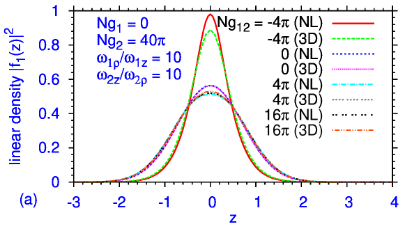
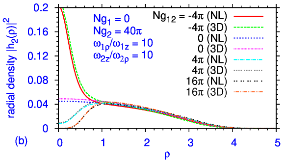
Figure 1: (Color online) Plot of (a) linear and (b) radial densities of a binary perpendicular cigar-disk mixture as obtained from the 3D GPE (3) and (4) (3D) and the reduced 1D-2D BNLSE (28) and (29) (NL) in dimensionless units for $Ng_{1}=0$ and $Ng_{2}=40\pi$ for different $Ng_{12}$. Parameters used: $m_{1}=m_{2}=\hbar=1$, $\omega_{1\rho}=\omega_{2z}=10,\omega_{1z}=\omega_{2\rho}=1,$ $a_{1z}=a_{2\rho}=1$, and $a_{1\rho}=a_{2z}=1/\sqrt{10}$. Both densities are normalized to unity.

To keep the algebra under control, we work in dimensionless units and set $m_{1}=m_{2}=\hbar=1$ and take $N_{1}=N_{2}=N$. For the cigar-shaped BEC we take $\omega_{1\rho}=10$ and $\omega_{1z}=1$; for the disk-shaped BEC we take $\omega_{2z}=10$, and $\omega_{2\rho}=1$. For the cigar-shaped BEC 1, the harmonic oscillator lengths are $a_{1z}\equiv\sqrt{\hbar/(m\omega_{1z})}=1$ and $a_{1\rho}\equiv\sqrt{\hbar/(m\omega_{1\rho})}=1/\sqrt{10}$. For the disk-shaped BEC 2, the harmonic oscillator lengths are $a_{2z}\equiv\sqrt{\hbar/(m\omega_{2z})}=1/\sqrt{10}$ and $a_{2\rho}\equiv\sqrt{\hbar/(m\omega_{2\rho})}=1$. The linear and radial densities are calculated from the solution of Eqs. (3) and (4) via

$$|f_{1}(z)|^{2}=2\pi\int_{0}^{\infty}\rho d\rho|\psi_{1}({\bf r})|^{2},$$ (53)

$$|h_{2}(\rho)|^{2}=\int_{-\infty}^{\infty}dz|\psi_{1}({\bf r})|^{2},$$ (54)

to be compared with the solutions of Eqs. (28) and (29).

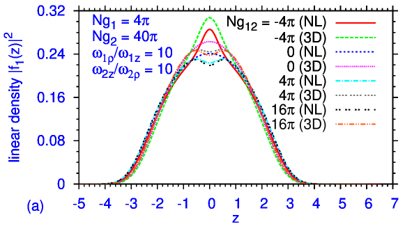
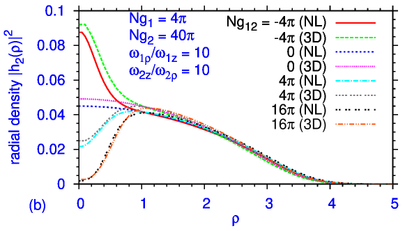
Figure 2: (Color online) The same as in Fig. 1 for $Ng_{1}=4\pi$ and $Ng_{2}=40\pi$.

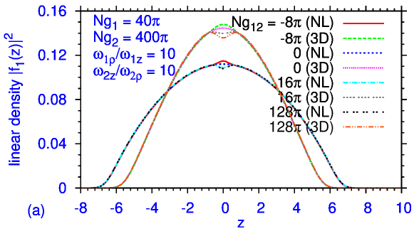
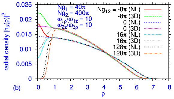
Figure 3: (Color online) The same as in Fig. 1 for $Ng_{1}=4\pi$ and $Ng_{2}=400\pi$.

To solve the coupled GPEs in three and reduced dimensions we employ the split-step Crank-Nicolson discretization technique murug with real and imaginary time propagation. We essentially use the Fortran programs provided in Ref. murug . The convergence of the numerical result was tested by varying the space (typically $\sim$ 0.05) and time (typically $\sim$ 0.001) steps and the total number of spatial and temporal discretization points.

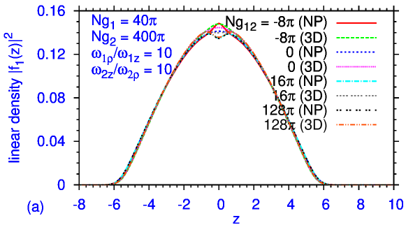
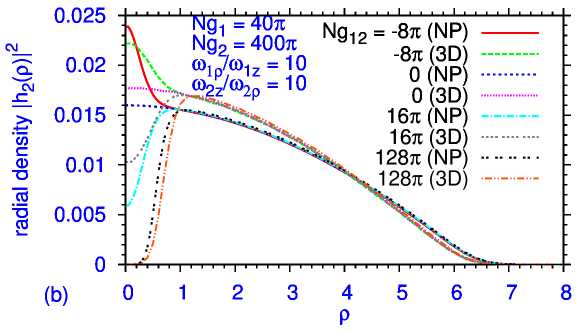
Figure 4: (Color online) The same as in Fig. 3 obtained using the reduced BNPSEs (III.2) $-$ (III.2) (NP).

IV.1 Stationary States

In Figs. 1 (a) and (b) we plot the linear and radial densities $|f_{1}(z)|^{2}$ and $h_{2}(\rho)|^{2}$, respectively, obtained from the 3D equations (3) and (4) as well as the BNLSE (28) and (29) for $Ng_{1}=0$ and $Ng_{2}=40\pi$ and for different $Ng_{12}$. In this case in the absence of coupling ($g_{12}=0$) the two linear densities are identical and the two radial densities very close to each other. The BNLSE (28) and (29) provide a faithful representation of the densities even in the presence of coupling as can be seen from Fig. 1.

In Figs. 2 (a) and (b) we plot the linear and radial densities $|f_{1}(z)|^{2}$ and $h_{2}(\rho)|^{2}$, respectively, as in Fig. 1 (a) and (b), for $Ng_{1}=4\pi$ and $Ng_{2}=40\pi$. In this case even for $g_{12}=0$, there is some difference between the results of the binary 3D GPE and the BNLSE. This difference is consistent with the previous studies sala1 ; camilo . The agreement between the densities obtained from the binary 3D GPE and the BNLSE continues to be good. The small discrepancy between the results of the binary 3D GPE and the BNLSE continues as a nonzero $g_{12}$ is introduced. This discrepancy does not increase as $g_{12}$ is increased to moderate values as we see from Fig. 2. In Figs. 3 (a) and (b) we plot the linear and radial densities for $Ng_{1}=40\pi$ and $Ng_{2}=400\pi$. In this case there is a larger difference between the results of 3D and reduced 1D-2D models. What is interesting is that the agreement between the results of the two models does not deteriorate with the increase of $g_{12}$ up to $128\pi$.

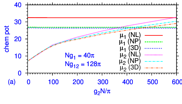
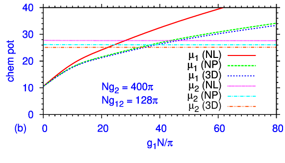
Figure 5: (Color online) (a) Chemical potential of the two components $\mu_{1}$ and $\mu_{2}$ calculated using the 3D GPE (3) and (4) (3D), the reduced BNPSEs (III.2) $-$ (III.2) (NP), and the reduced BNLSE (28) and (29) (NL) versus $g_{2}N/\pi$ for $Ng_{1}=40\pi,N_{g}{12}=128\pi$. (b) Chemical potential of the two components $\mu_{1}$ and $\mu_{2}$ calculated using the 3D GPE (3) and (4) (3D), the reduced BNPSEs (III.2) $-$ (III.2) (NP), and the reduced BNLSE (28) and (29) (NL) versus $g_{1}N/\pi$ for $Ng_{2}=400\pi,Ng_{12}=128\pi$.

From the results displayed in Figs. 1 $-$ 3 we find that the BNLSE (28) and (29) provide an excellent account of the actual state of affairs, when compared with the full 3D binary GPE (3) and (4), specially for small nonlinearities $Ng_{1}$ and $Ng_{2}$.

We next attempt an improvement over the BNLSE (28) and (29) of Sec. II by applying BNPSE of Sec. III. In other words, we attempt a solution of Eqs. (III.2) $-$ (III.2), in place of Eqs. (28) and (29), to reduce the discrepancy noted in Figs. 3 (a) and (b) between the results of the 3D and BNLSE. The results so obtained are plotted in Figs. 4 (a) and (b) for $Ng_{1}=40\pi$ and $Ng_{2}=400\pi$, which show a significant improvement over the results in Figs. 3 (a) and (b). The large discrepancy between the results of the 3D binary GPE and the BNLSE for the linear density of component 1 has virtually disappeared in Fig. 4 (a) and that for the radial density of component 2 is significantly reduced in Fig. 4 (b). This shows that although the results from the effective BNLSE of Sec. II are quite good for small nonlinearities, significant improvement can be obtained from the BNPSE of Sec. III, especially for larger values of nonlinearities.

Finally, we consider the chemical potential $\mu_{1}$ and $\mu_{2}$ of the two components calculated using the 3D binary GPE (3) and (4), the BNPSE (III.2) $-$ (III.2) as well as the BNLSE (28) $-$ (29). The equations for the chemical potentials are obtained by replacing the time derivative $i\hbar\partial_{t}$ by $\mu_{1}$ and $\mu_{2}$, respectively, in the dynamical equations for component 1 and 2, respectively. The chemical potentials are plotted in Fig. 5 (a) versus $g_{1}N/\pi$ for $Ng_{2}=400\pi$ and $Ng_{12}=128\pi$. In Fig. 5 (b) we plot the chemical potentials versus $g_{2}N/\pi$ for $Ng_{1}=40\pi$ and $Ng_{12}=128\pi$. The chemical potentials obtained from the BNLSE (28) $-$ (29) are good but those calculated from the BNPSE (III.2) $-$ (III.2) are better approximations to the results obtained from the 3D binary GPE (3) and (4) in all cases.

IV.2 Dynamics

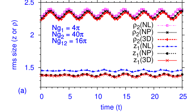
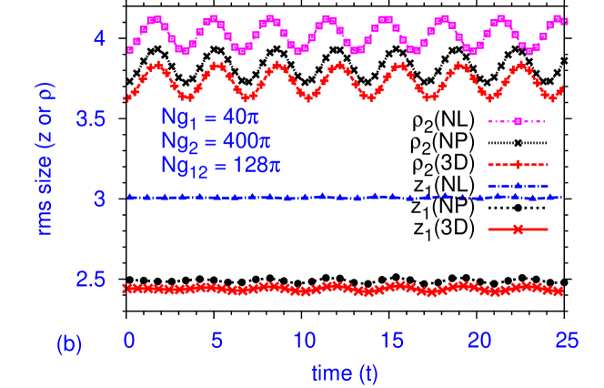
Figure 6: (Color online) Evolution of axial and radial rms sizes of the cigar- and disk-shaped components of the binary BEC after a sudden reduction of the radial angular frequency of the disc-shaped component by $5\%$, for the nonlinearities (a) $Ng_{1}=4\pi,Ng_{2}=40\pi,Ng_{12}=16\pi$ and (b) $Ng_{1}=40\pi,Ng_{2}=400\pi,Ng_{12}=128\pi$. The cigar-shaped BEC is perpendicular to the disk-shaped BEC.

Now we investigate if the reduced equation presented here can satisfactorily describe the dynamics of the perpendicular 1D-2D system. For this purpose first we consider the coupled system presented in Figs. 2 (a) and (b) with $Ng_{1}=4\pi,Ng_{2}=40\pi,$ and $Ng_{12}=16\pi$. After the stationary condensate is created during time evolution of the numerical routine using real-time propagation, we reduce the radial angular frequency of the disk-shaped quasi-2D BEC suddenly by 5$\%$ (the new angular frequencies being $\omega_{1\rho}=\omega_{2z}=10,\omega_{1z}=1,\omega_{2\rho}=0.95,$) and study the subsequent dynamical evolution of the system. The relevant dynamics is best illustrated by plotting the evolution of the rms axial size of the cigar-shaped quasi-1D BEC and the rms radial size of the disk-shaped quasi-2D BEC in Fig. 6 (a) and (b) for two sets of nonlinearities exhibited in Figs. 2 and 3. Here we show the results of the 3D GPE (3) and (4) (3D), the reduced BNPSEs (III.2) $-$ (III.2) (NP), and the reduced BNLSE (28) and (29) (NL). For both sets of nonlinearities illustrated in Figs. 6 (a) $Ng_{1}=4\pi,Ng_{2}=40\pi,Ng_{12}=16\pi$ and (b) $Ng_{1}=40\pi,Ng_{2}=400\pi,Ng_{12}=128\pi$, the NP reduction produced far better results compared to the NL reduction. In both cases the angular frequency of the quasi-2D disk-shaped BEC was modified and both the NL and NP schemes as well as the full 3D calculation exhibited sinusoidal oscillation for the axial size of the disk-shaped BEC right from $t=0$. It took some five units of time for similar sinusoidal oscillation to initiate in the unperturbed cigar-shaped component due to the non-zero coupling term $g_{12}$. The oscillations in rms sizes in the NP scheme were always in phase with those of the full 3D calculation. But for larger nonlinearity and at large times the oscillations in rms sizes in the NL scheme are not always in phase with those of the full 3D calculation. The differences between the rms sizes of the NL and NP schemes compared to the full 3D calculation were consequences of the same differences, existing at $t=0$, in the corresponding stationary results in the absence of any perturbation in the angular frequency.

V SUMMARY

In this paper we derived and studied simple binary reduced non-polynomial Schrödinger equations (BNPSEs) for the description of a binary BEC where the two components subject to distinct trap symmetries belong to two different spatial dimensions. We considered three possibilities: the first component is in 3D and the second in (a) 1D (cigar shape) or (b) 2D (disk shape), and (c) the first component is in 1D and the second in 2D. The 1D and 2D configurations were achieved in an axially-symmetric setting with a strong harmonic trap in the transverse radial and axial directions, respectively. The BNPSEs were obtained by a Lagrangian variational scheme after approximating the spatial wave-function component in the transverse direction by a generic Gaussian function. A simpler set of reduced equations, the BNLSE with power-law nonlinearity, were obtained with a simple ansatz for the 3D wave function where the wave-function component in the transverse direction is taken to be the ground state in the corresponding harmonic trap.

We tested the accuracy of the reduction scheme above by numerically solving the 3D binary GPE in the coupled 1D-2D case where the cigar-shaped component is in the $z$ direction and the disk-shaped component lie in the $(x,y)$ plane. We calculated the density profiles and the chemical potentials of the two components. For smaller values of inter- and intra-species nonlinearities, the BNLSE (28) and (29) with power-law nonlinearity produced results for density and chemical potential in good agreement with the binary 3D GPE. For larger nonlinearities the BNPSE (III.2) $-$ (III.2) produced significant improvement over the BNLSE (28) and (29). We also studied small oscillation of the binary 1D-2D BEC, initiated by a sudden change of the radial angular frequency of the 2D component. For larger nonlinearities and large times, the BNPSE (III.2) $-$ (III.2) produced better results for dynamics compared with the BNLSE (28) and (29). To conclude, the BNLSE (28) and (29) as well as the BNPSE (III.2) $-$ (III.2) are shown to be very useful to investigate a binary 1D-2D BEC, where the cigar-shaped BEC is perpendicular to the disk-shaped one. Similar reduced equations are derived for other symmetries, such as the 1D-3D and 2D-3D cases as well as the 1D-2D case where the cigar-shaped BEC is in the plane of the disk-shaped one.

References

• (1) L. Pitaevskii and S. Stringari, Bose-Einstein Condensation (Clarendon Press: Oxford, 2003).
• (2) A. J. Leggett, Quantum Liquids. Bose Condensation and Cooper Pairing in Condensed-Matter Systems (Oxford Univ. Press, Oxford, 2006).
• (3) V. M. Pérez-García, H. Michinel, and H. Herrero, Phys. Rev. A 57, 3837 (1998).
• (4) A. D. Jackson, G. M. Kavoulakis, and C. J. Pethick, Phys. Rev. A 58, 2417 (1998).
• (5) L. Salasnich, A. Parola, and L. Reatto, Phys. Rev. A 65, 043614 (2002); L. Salasnich, Laser Phys. 12, 198 (2002).
• (6) P. Massignan and M. Modugno, Phys. Rev. A 67, 023614 (2003); M. Modugno, C. Tozzo, and F. Dalfovo, Phys. Rev. A 70, 043625 (2004); C. Tozzo, M. Kramer, and F. Dalfovo, Phys. Rev. A 72 023613 (2005): M. Modugno, Phys. Rev. A 73, 013606 (2006).
• (7) A. Munoz Mateo and V. Delgado, Phys. Rev. A 75, 063610 (2007); Phys. Rev. A 77, 013617 (2008); Ann. Phys. 324, 709 (2009).
• (8) C. A. G. Buitrago and S. K. Adhikari, J. Phys. B 42, 215306 (2009).
• (9) G. Theocharis, P. G. Kevrekidis, M. K. Oberthaler, and D. J. Frantzeskakis, Phys. Rev. A 76, 045601 (2007); A. Weller, J. P. Ronzheimer, C. Gross, J. Esteve, M. K. Oberthaler, D. J. Frantzeskakis, G. Theocharis, and P. G. Kevrekidis, Phys. Rev. Lett. 101, 130401 (2008).
• (10) M. L. Chiofalo and M. P. Tosi, Phys. Lett. A 268, 406 (2000); A. M. Kamchatnov and V. S. Shchesnovich, Phys. Rev. A 70, 023604 (2004); W. Zhang and L. You, Phys. Rev. A 71, 025603 (2005); F. K. Abdullaev and R. Galimzyanov, J. Phys. B 36, 1099 (2003).
• (11) L. Salasnich, A. Parola, and L. Reatto, Phys. Rev. A 66, 043603 (2002); L. Salasnich, Phys. Rev. A 70, 053617 (2004); L. Salasnich, A. Parola and L. Reatto, Phys. Rev. A 70 013606 (2004); A. Parola, L. Salasnich, R. Rota, and L. Reatto, Phys. Rev. A 72, 063612 (2005).
• (12) A. Maluckov, L. Hadzievski, B. A. Malomed, and L. Salasnich, Phys. Rev. A 78, 013616 (2008); L. Salasnich, J. Phys. A: Math. Theor. 42, 335205 (2009); G. Gligoric, A. Maluckov, L. Hadzievski, L. Salasnich, and B.A. Malomed, Chaos 19, 043105 (2009).
• (13) L. Salasnich and B. A. Malomed, Phys. Rev. A 79, 053620 (2009).
• (14) S. K. Adhikari and L. Salasnich, New J. Phys. 11, 023011 (2009).
• (15) Y.E. Kim and A.L. Zubarev, Phys. Rev. A 70, 033612 (2004); N. Manini and L. Salasnich, Phys. Rev. A 71, 033625 (2005); G. Diana, N. Manini, L. Salasnich, Phys. Rev. A 73, 065601 (2006); W. Wen and G.X. Huang, Phys. Rev. A 79, 023605 (2009); S. K. Adhikari and L. Salasnich, Phys. Rev. A 78, 043616 (2008); S. K. Adhikari, Laser Phys. Lett. 6, 901 (2009); Phys. Rev. A 77 045602 (2008); J. Phys. B 43, 085304 (2010); L. Salasnich and F. Toigo, Phys. Rev. A 78, 053626 (2008); L. Salasnich, F. Ancilotto, and F. Toigo, Laser Phys. Lett. 7, 78 (2010).
• (16) S. K. Adhikari and L. Salasnich, Phys. Rev. A 80, 023606 (2009); S. K. Adhikari, ibid. 81, 043636 (2010); Y. Cheng and S. K. Adhikari, ibid. 81, 023620 (2010); 82, 013631 (2010); Laser Phys. Lett. in press (2010) (arXiv:1006.4277).
• (17) G. Lamporesi, J. Catani, G. Barontini, Y. Nishida, M. Inguscio, and F. Minardi, Phys. Rev. Lett. 104, 153202 (2010).
• (18) L. Salasnich and B. A. Malomed, Phys. Rev. A 74, 053610 (2006); L. Salasnich, B. A. Malomed, and F. Toigo, Phys. Rev. A 81, 045603 (2010).
• (19) G.P. Kevrekidis, D.J. Frantzeskakis, R. Carretero-González (Eds.), Emergent Nonlinear Phenomena in Bose-Einstein Condensates (Springer, Berlin, 2008).
• (20) P. Muruganandam and S. K. Adhikari, Comput. Phys. Commun. 180, 1888 (2009).
• (21) P. Muruganandam and S. K. Adhikari, J. Phys. B 36, 2501 (2003); S. K. Adhikari and P. Muruganandam, J. Phys. B 35, 2831 (2002).