A Correction Function Method for Poisson Problems with Interface Jump Conditions.
Abstract
In this paper we present a method to treat interface jump conditions for constant coefficients Poisson problems that allows the use of standard “black box” solvers, without compromising accuracy. The basic idea of the new approach is similar to the Ghost Fluid Method (GFM). The GFM relies on corrections applied on nodes located across the interface for discretization stencils that straddle the interface. If the corrections are solution-independent, they can be moved to the right-hand-side (RHS) of the equations, producing a problem with the same linear system as if there were no jumps, only with a different RHS. However, achieving high accuracy is very hard (if not impossible) with the “standard” approaches used to compute the GFM correction terms.
In this paper we generalize the GFM correction terms to a correction function, defined on a band around the interface. This function is then shown to be characterized as the solution to a PDE, with appropriate boundary conditions. This PDE can, in principle, be solved to any desired order of accuracy. As an example, we apply this new method to devise a 4 order accurate scheme for the constant coefficients Poisson equation with discontinuities in 2D. This scheme is based on (i) the standard 9-point stencil discretization of the Poisson equation, (ii) a representation of the correction function in terms of bicubics, and (iii) a solution of the correction function PDE by a least squares minimization. Several applications of the method are presented to illustrate its robustness dealing with a variety of interface geometries, its capability to capture sharp discontinuities, and its high convergence rate.
keywords:
Poisson equation , interface jump condition , Ghost Fluid method , Gradient augmented level set method , High accuracy , Hermite cubic splinePACS:
47.11-j , 47.11.BcMSC:
[2010] 76M20 , 35N061 Introduction.
1.1 Motivation and background information.
In this paper we present a new and efficient method to solve the constant coefficients Poisson equation in the presence of discontinuities across an interface, with a high order of accuracy. Solutions of the Poisson equation with discontinuities are of fundamental importance in the description of fluid flows separated by interfaces (e.g. the contact surfaces for immiscible multiphase fluids, or fluids separated by a membrane) and other multiphase diffusion phenomena. Over the last three decades, several methods have been developed to solve problems of this type numerically [1, 2, 3, 4, 5, 6, 7, 8, 9, 10, 11, 12, 13, 14, 15, 16, 17]. However, obtaining a high order of accuracy still poses great challenges in terms of complexity and computational efficiency.
When the solution is known to be smooth, it is easy to obtain highly accurate finite-difference discretizations of the Poisson equation on a regular grid. Furthermore, these discretizations commonly yield symmetric and banded linear systems, which can be inverted efficiently [18]. On the other hand, when singularities occur (e.g. discontinuities) across internal interfaces, some of the regular discretization stencils will straddle the interface, which renders the whole procedure invalid.
Several strategies have been proposed to tackle this issue. Peskin [1] introduced the Immersed Boundary Method (IBM) [1, 10], in which the discontinuities are re-interpreted as additional (singular) source terms concentrated on the interface. These singular terms are then “regularized” and appropriately spread out over the regular grid — in a “thin” band enclosing the interface. The result is a first order scheme that smears discontinuities. In order to avoid this smearing of the interface information, LeVeque and Li [3] developed the Immersed Interface Method (IIM) [3, 4, 11, 13], which is a methodology to modify the discretization stencils, taking into consideration the discontinuities at their actual locations. The IIM guarantees second order accuracy and sharp discontinuities, but at the cost of added discretization complexity and loss of symmetry.
The new method advanced in this paper builds on the ideas introduced by the Ghost Fluid Method (GFM) [19, 6, 7, 9, 8, 12, 14]. The GFM is based on defining both actual and “ghost” fluid variables at every node on a narrow band enclosing the interface. The ghost variables work as extensions of the actual variables across the interface — the solution on each side of the interface is assumed to have a smooth extension into the other side. This approach allows the use of standard discretizations everywhere in the domain. In most GFM versions, the ghost values are written as the actual values, plus corrections that are independent of the underlying solution to the Poisson problem. Hence, the corrections can be pre-computed, and moved into the source term for the equation. In this fashion the GFM yields the same linear system as the one produced by the problem without an interface, except for changes in the right-hand-side (sources) only, which can then be inverted just as efficiently.
The key difficulty in the GFM is the calculation of the correction terms, since the overall accuracy of the scheme depends heavily on the quality of the assigned ghost values. In [6, 7, 9, 8, 12] the authors develop first order accurate approaches to deal with discontinuities. In the present work, we show that for the constant coefficients Poisson equation we can generalize the GFM correction term (at each ghost point) concept to that of a correction function defined on a narrow band enclosing the interface. Hence we call this new approach the Correction Function Method (CFM). This correction function is then shown to be characterized as the solution to a PDE, with appropriate boundary conditions on the interface — see § 4. Thus, at least in principle, one can calculate the correction function to any order of accuracy, by designing algorithms to solve the PDE that defines it. In this paper we present examples of 2 and 4 order accurate schemes (to solve the constant coefficients Poisson equation, with discontinuities across interfaces, in 2D) developed using this general framework.
A key point (see § 5) in the scheme developed here is the way we solve the PDE defining the correction function. This PDE is solved in a weak fashion using a least squares minimization procedure. This provides a flexible approach that allows the development of a robust scheme that can deal with the geometrical complications of the placement of the regular grid stencils relative to the interface. Furthermore, this approach is easy to generalize to 3D, or to higher orders of accuracy.
1.2 Other related work.
It is relevant to note other developments to solve the Poisson equation under similar circumstances — multiple phases separated by interfaces — but with different interface conditions. The Poisson problem with Dirichlet boundary conditions, on an irregular boundary embedded in a regular grid, has been solved to second order of accuracy using fast Poisson solvers [19], finite volume [5], and finite differences [20, 21, 22, 23] approaches. In particular, Gibou et al. [21] and Jomaa and Macaskill [22] have shown that it is possible to obtain symmetric discretizations of the embedded Dirichlet problem, up to second order of accuracy. Gibou and Fedkiw [23] have developed a fourth order accurate discretization of the problem, at the cost of giving up symmetry. More recently, the same problem has also been solved, to second order of accuracy, in non-graded adaptive Cartesian grids by Chen et al. [24]. Furthermore, the embedded Dirichlet problem is closely related to the Stefan problem modeling dendritic growth, as described in [25, 26].
The finite-element community has also made significant progress in incorporating the IIM and similar techniques to solve the Poisson equation using embedded grids. In particular the works by Gong et al. [15], Dolbow and Harari [16], and Bedrossian et al. [17] describe second order accurate finite-element discretizations that result in symmetric linear systems. Moreover, in these works the interface (or boundary) conditions are imposed in a weak fashion, which bears some conceptual similarities with the CFM presented here, although the execution is rather different.
1.3 Interface representation.
Another issue of primary importance to multiphase problems is the representation of the interface (and its tracking in unsteady cases). Some authors (see [1, 19, 20]) choose to represent the interface explicitly, by tracking interface particles. The location of the neighboring particles is then used to produce local interpolations (e.g. splines), which are then applied to compute geometric information — such as curvature and normal directions. Although this approach can be quite accurate, it requires special treatment when the interface undergoes either large deformations or topological changes — such as mergers or splits. Even though we are not concerned with these issues in this paper, we elected to adopt an implicit representation, to avoid complications in future applications. In an implicit representation, the interface is given as the zero level of a function that is defined everywhere in the regular grid — the level set function [27]. In particular, we adopted the Gradient-Augmented Level Set (GA-LS) method [28]. With this extension of the level set method, we can obtain highly accurate representations of the interface, and other geometric information, with the additional advantage that this method uses only local grid information. We discuss the question of interface representation in more detail in § 5.6.
1.4 Organization of the paper.
The remainder of the paper is organized as follows. In § 2 we introduce the Poisson problem that we seek to solve. In § 3 the basic idea behind the solution method, and its relationship to the GFM, are explored. Next, in § 4, we introduce the concept of the correction function and show how it is defined by a PDE problem. In § 5 we apply this new framework to build a 4 order accurate scheme in 2D. Since the emphasis of this paper is on high-order schemes, we describe the 2 order accurate scheme in appendix C. Next, in § 6 we demonstrate the robustness and accuracy of the 2D scheme by applying it to several example problems. The conclusions are in § 7. In appendix A we review some background material, and notation, on bicubic interpolation. Finally, in appendix B we discuss some technical issues regarding the construction of the sets where the correction function is solved for.
2 Definition of the problem.
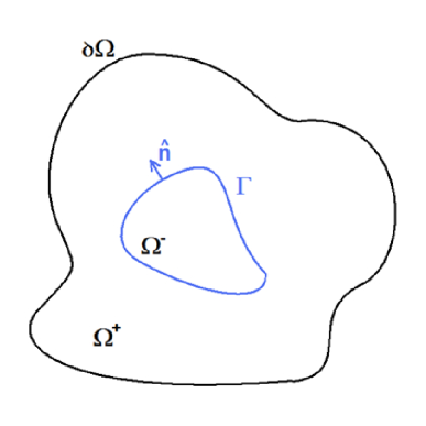
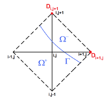
Our objective is to solve the constant coefficients Poisson’s equation in a domain in which the solution is discontinuous across a co-dimension 1 interface , which divides the domain into the subdomains and , as illustrated in figure 1. We use the notation and to denote the solution in each of the subdomains. Let the discontinuities across be given in terms of two functions defined on the interface: for the jump in the function values, and for the jump in the normal derivatives. Furthermore, assume Dirichlet boundary conditions on the “outer” boundary (see figure 1). Thus the problem to be solved is
| (1a) | ||||||
| (1b) | ||||||
| (1c) | ||||||
| (1d) | ||||||
where
| (2a) | ||||||
| (2b) | ||||||
Throughout this paper, is the spatial vector (where , or ), and is the Laplacian operator defined by
| (3) |
Furthermore,
| (4) |
denotes the derivative of in the direction of , the unit vector normal to the interface pointing towards (see figure 1).
It is important to note that our method focuses on the discretization of the problem in the vicinity of the interface only. Thus, the method is compatible with any set of boundary conditions on , not just Dirichlet.
3 Solution method – the basic idea.
To achieve the goal of efficient high order discretizations of Poisson equation in the presence of discontinuities, we build on the idea of the Ghost Fluid Method (GFM). In essence, we use a standard discretization of the Laplace operator (on a domain without an interface ) and modify the right-hand-side (RHS) to incorporate the jump conditions across . Thus, the resulting linear system can be inverted as efficiently as in the case of a solution without discontinuities.
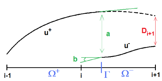
Let us first illustrate the key concept in the GFM with a simple example, involving a regular grid and the standard second order discretization of the 1D analog of the problem we are interested in. Thus, consider the problem of discretizing the equation in some interval , where is discontinuous across some point — hence (respectively ) is the domain (respectively ). Then, see figure 2, when trying to approximate at a grid point such that , we would like to write
| (5) |
where is the grid spacing. However, we do not have information on , but rather on . Thus, the idea is to estimate a correction for , to recover , such that Eq. (5) can be applied:
| (6) |
where is the correction term. Now we note that, if can be written as a correction that is independent on the solution , then it can be moved to the RHS of the equation, and absorbed into . That is
| (7) |
This allows the solution of the problem with prescribed discontinuities using the same discretization as the one employed to solve the simpler problem without an interface — which leads to a great efficiency gain.
Remark 1.
The error in estimating is crucial in determining the accuracy of the final discretization. Liu, Fedkiw, and Kang [9] introduced a dimension-by-dimension linear extrapolation of the interface jump conditions, to get a first order approximation for . Our new method is based on generalizing the idea of a correction term to that of a correction function, for which we can write an equation. One can then obtain high accuracy representations for by solving this equation, without the complications into which dimension-by-dimension (with Taylor expansions) approaches run into.
Remark 2.
An additional advantage of the correction function approach is that can be calculated at any point near the interface . Hence it can be used with any finite differences discretization of the Poisson equation, without regard to the particulars of its stencil (as would be the case with any approach based on Taylor expansions).
4 The correction function and the equation defining it.
As mentioned earlier, the aim here is to generalize the correction term concept to that of a correction function, and then to find an equation (a PDE, with appropriate boundary conditions) that uniquely characterizes the correction function. Then, at least in principle, one can design algorithms to solve the PDE in order to obtain solutions to the correction function of any desired order of accuracy.
Let us begin by considering a small region enclosing the interface , defined as the set of all the points within some distance of , where is of the order of the grid size . As we will see below, we would like to have as small as possible. On the other hand, has to include all the points where the CFM requires corrections to be computed, which means111For the particular discretization of the Laplace operator that we use in this paper. that cannot be smaller than . In addition, algorithmic considerations (to be seen later) force to be slightly larger than this last value.
Next, we assume we that can extrapolate both and , so that they are valid everywhere within , in such a way that they satisfy the Poisson equations
| (8a) | ||||||
| (8b) | ||||||
where and are smooth enough (see remark 3 below) extensions of the source term to . In particular, notice that the introduction of and allows the possibility of the source term changing (i.e. a discontinuous source term) across . The correction function is then defined by .
Taking the difference between the equations in (8), and using the jump conditions (1b-1c), yields
| (9a) | ||||||
| (9b) | ||||||
| (9c) | ||||||
This achieves the aim of having the correction function defined by a set of equations, with some provisos — see remark 4 below. Note that:
-
1.
If , for , then , for .
- 2.
Remark 3.
The smoothness requirement on and is tied up to how accurate an approximation to the correction term is needed. For example, if a 4 order algorithm is used to find , this will (generally) necessitate to be at least for the errors to actually be 4 order. Hence, in this case, must be .
Remark 4.
Equation (9) is an elliptic Cauchy problem for in . In general, such problems are ill-posed. However, we are seeking for solutions within the context of a numerical approximation where
-
1.
There is a frequency cut-off in both the data and , and the description of the curve .
-
2.
We are interested in the solution only a small distance away from the interface , where this distance vanishes simultaneously with the inverse of the cut-off frequency in point (a).
What (a) and (b) mean is that the arbitrarily large growth rate for arbitrarily small perturbations, which is responsible for the ill-posedness of the Cauchy problem in Eq. (9), does not occur within the special context where we need to solve the problem. This large growth rate does not occur because, for the solutions of the Poisson equation, the growth rate for a perturbation of wave number along some straight line, is given by — where is the distance from the line. However, by construction, in the case of interest to us is bounded.
Remark 5.
Let us be more precise, and define a number characterizing how well posed the discretized version of Eq. (9) is, by
where growth is defined relative to the size of a perturbation to the solution on the interface. This number is determined by (the “radius” of ) as the following calculation shows: First of all, there is no loss of generality in assuming that the interface is flat, provided that the numerical grid is fine enough to resolve . In this case, let us introduce an orthogonal coordinate system on , and let be the signed distance to (say, in ). Expanding the perturbations in Fourier modes along the interface, the typical mode has the form
where is the Fourier wave vector, and . The shortest wave-length that can be represented on a grid with mesh size corresponds to . Hence, we obtain the estimate
for the maximum growth rate.
Remark 6.
Clearly, is intimately related to the condition number for the discretized problem — see § 5. In fact, at leading order, the two numbers should be (roughly) proportional to each other — with a proportionality constant that depends on the details of the discretization. For the discretization used in this paper (described further below), , which leads to the rough estimate . On the other hand, the observed condition numbers vary between 5,000 and 10,000. Hence, the actual condition numbers are only slightly higher than for the ranges of grid sizes that we used (we did not explore the asymptotic limit ).
Remark 7.
Equation (9) depends on the known inputs for the problem only. Namely: , , , and . Consequently does not depend on the solution . Hence, after solving for , we can use a discretization for that does not involve the interface: Whenever is discontinuous, we evaluate where the correction is needed, and transfer these values to the RHS.
Remark 8.
When developing an algorithm for a linear Cauchy problem, such as the one in Eq. (9), the two key requirements are consistency and stability. In particular, when the solution depends on the “initial conditions” globally, stability (typically) imposes stringent constraints on the “time” step for any local (explicit) scheme. This would seem to suggest that, in order to solve Eq. (9), a “global” (involving the whole domain ) method will be needed. This, however, is not true: because we need to solve Eq. (9) for one “time” step only — i.e. within an distance from , stability is not relevant. Hence, consistency is enough, and a fully local scheme is possible. In the algorithm described in § 5 we found that, for (local) quadrangular patches, the Cauchy problem leads to a well behaved algorithm when the length of the interface contained in each patch is of the same order as the diagonal length of the patch. This result is in line with the calculation in remark 5: we want to keep the “wavelength” (along ) of the perturbations introduced by the discretization as long as possible. In particular, this should then minimize the condition number for the local problems — see remark 6.
5 A 4 Order Accurate Scheme in 2D.
5.1 Overview.
In this section we use the general ideas presented earlier to develop a specific example of a 4 order accurate scheme in 2D. Before proceeding with an in-depth description of the scheme, we highlight a few key points:
- 1.
-
2.
We approximate using bicubic interpolations (bicubics), each valid in a small neighborhood of the interface. This guarantees local 4 order accuracy with only 12 interpolation parameters — see [28]. Each corresponds to a point in the grid at which the standard discretization of Poisson’s equation involves a stencil that straddles the interface .
-
3.
The domains are rectangular regions, each enclosing a portion of , and all the nodes where is needed to complete the discretization of the Poisson equation at the ()-th stencil. Each is a sub-domain of .
-
4.
Starting from (b) and (c), we design a local solver that provides an approximation to inside each domain .
-
5.
The interface is represented using the Gradient-Augmented Level Set approach — see [28]. This guarantees a local 4 order representation of the interface, as required to keep the overall accuracy of the scheme.
-
6.
In each , we solve the PDE in (9) in a least squares sense. Namely: First we define an appropriate positive quadratic integral quantity — Eq. (17) — for which the solution is a minimum (actually, zero). Next we substitute the bicubic approximation for the solution into , and discretize the integrals using Gaussian quadrature. Finally, we find the bicubic parameters by minimizing the discretized .
Remark 9.
Solving the PDE in a least squares sense is crucial, since an algorithm is needed that can deal with the myriad ways in which the interface can be placed relative to the fixed rectangular grid used to discretize Poisson’s equation. This approach provides a scheme that (i) is robust with respect to the details of the interface geometry, (ii) has a formulation that is (essentially) dimension independent — there are no fundamental changes from 2D to 3D, and (iii) has a clear theoretical underpinning that allows extensions to higher orders, or to other discretizations of the Poisson equation.
5.2 Standard Stencil.
We use the standard 4 order accurate 9-point discretization of Poisson’s equation222Notice that here we allow for the possibility of different grid spacings in each direction.:
| (10) |
where is the second order 5-point discretization of the Laplace operator:
| (11) |
and
| (12) | ||||
| (13) |
The terms and may be given analytically (if known), or computed using appropriate second order discretizations.
In the absence of discontinuities, Eq. (10) provides a compact 4 order accurate representation of Poisson’s equation. In the vicinity of the discontinuities at the interface , we define an appropriate domain , and compute the correction terms necessary to Eq. (10) — as described in detail next.
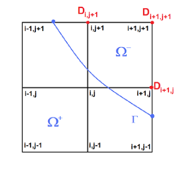
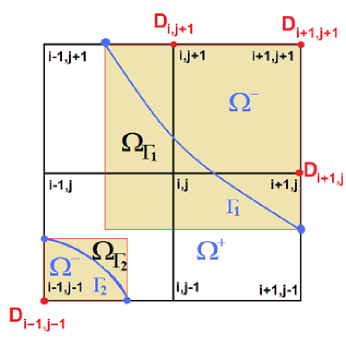
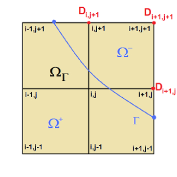
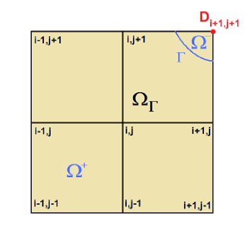
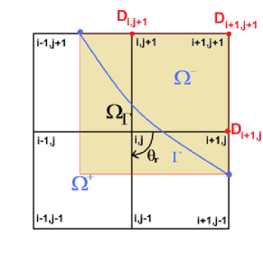
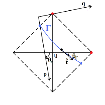
To understand how the correction terms affect the discretization, let us consider the situation depicted in figure 3. In this case, the node lies in while the nodes , , and are in . Hence, to be able to use Eq. (10), we need to compute , , and .
After having solved for where necessary (see § 5.3 and § 5.4), we modify Eq. (10) and write
| (14) |
which differs from Eq. (10) by the terms on the RHS only. Here the are the CFM correction terms needed to complete the stencil across the discontinuity at . In the particular case illustrated in figure 3, we have
| (15) |
Similar formulas apply for the other possible arrangements of the Poisson’s equation stencil relative to the interface .
5.3 Definition of .
There is some freedom on how to define . The basic requirements are
-
1.
should be a rectangle.
-
2.
the edges of should be parallel to the grid lines.
- 3.
-
4.
should contain all the nodes where is needed. For the example, in figure 3 we need to know , , and . Hence, in this case, should include the nodes , , and .
-
5.
should contain a segment of , with a length that is as large as possible — i.e. comparable to the length of the diagonal of . This follows from the calculation in remark 5, which indicates that the wavelength of the perturbations (along ) introduced by the discretization should be as long as possible. This should then minimize the condition number for the local problem — see remark 6.
Requirements (i) and (ii) are needed for algorithmic convenience only, and do not arise from any particular argument in § 4. Thus, in principle, this convenience could be traded for improvements in other areas — for example, for better condition numbers for the local problems, or for additional flexibility in dealing with complex geometries. However, for simplicity, in this paper we enforce (i) and (ii). As explained earlier (see remark 9), we solve Eq. (9) in a least squares sense. Hence integrations over are required. It is thus useful to keep as simple as possible.
A discussion of various aspects regarding the proper definition of can be found in appendix B. For instance, the requirement in item (ii) is convenient only when an implicit representation of the interface is used. Furthermore, although the definition of presented here proved robust for all the applications of the 4 order accurate scheme (see § 6), there are specific geometrical arrangements of the interface for which (ii) results in extremely elongated . These elongated geometries can have negative effects on the accuracy of the scheme. We noticed this effect in the 2 order accurate version of the method described in appendix C. These issues are addressed by the various algorithms (of increasing complexity) presented in appendix B.
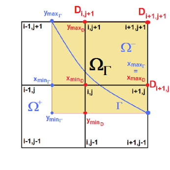
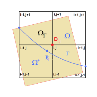
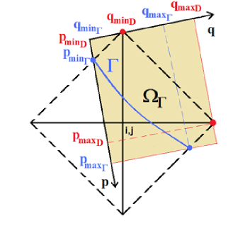
With the points above in mind, here (for simplicity) we define as the smallest rectangle that satisfies the requirements in (i), (ii), (iv), and (v) — then (iii) follows automatically. Hence can be constructed using the following three easy steps:
-
1.
Find the coordinates () and () of the smallest rectangle satisfying condition (ii), which completely encloses the section of the interface contained by the region covered by the 9-point stencil.
-
2.
Find the coordinates () and () of the smallest rectangle satisfying condition (ii), which completely encloses all the nodes at which needs to be known.
-
3.
Then is the smallest rectangle that encloses the two previous rectangles. Its edges are given by
(16a) (16b) (16c) (16d)
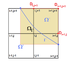
Figure 4 shows an example of defined using these specifications.
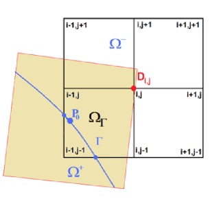
Remark 10.
Notice that for each node next to the interface we construct a domain . When doing so, we allow the domains to overlap. For example, the domain shown in figure 4 is used to determine . It should be clear that (used to determine ), and (used to determine ), each will overlap with .
The consequence of these overlaps is that different computed values for at the same node can (in fact, will) happen — depending on which domain is used to solve the local Cauchy problem. However, because we solve for — within each — to 4 order accuracy, any differences that arise from this multiple definition of lie within the order of accuracy of the scheme. Since it is convenient to keep the computations local, the values of resulting from the domain , are used to evaluate the correction term .
Remark 11.
While rare, cases where a single interface crosses the same stencil multiple times can occur. In § 6.3 we present such an example. A simple approach to deal with situations like this is as follows: First associate each node where the correction function is needed to a particular piece of interface crossing the stencil (say, the closest one). Then define one for each of the individual pieces of interface crossing the stencil.
For example, figure 5(a) depicts a situation where the stencil is crossed by two pieces of the same interface ( and ), with needed at the nodes , , , and . Then, first associate: (i) , , and to , and (ii) to . Second, define
-
1.
is the smallest rectangle, parallel to the grid lines, that includes and the nodes , , and .
-
2.
is the smallest rectangle, parallel to the grid lines, that includes and the node .
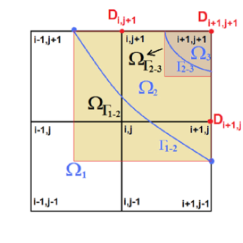
(a) (b)
After the multiple are defined within a given stencil, the local Cauchy problem is solved for each separately. For example, in the case shown in figure 5(a), the solution for inside is done completely independent of the solution for inside . The decoupling between multiple crossings renders the CFM flexible and robust enough to handle complex geometries without any special algorithmic considerations.
Remark 12.
When multiple distinct interfaces are involved, a single stencil can be crossed by different interfaces – e.g.: see § 6.5 and § 6.6. This situation is similar to the one described in remark 11, but with an additional complication: there may occur distinct domain regions that are not separated by an interface, but rather by a third (or more) regions between them. An example is shown in figure 5(b), where and are not part of the same interface. Here is the interface between and , while is the interface between and . There is no interface separating from , hence no jump conditions between these regions are provided. Nonetheless, is needed at .
Situations such as these can be easily handled by noticing that we can distinguish between primary (e.g. and ) and secondary correction functions, which can be written in terms of the primary functions (e.g. ) and need not be computed directly. Hence we can proceed exactly as in remark 11, except that we have to make sure that the intersections of the regions where the primary correction functions are computed include the nodes where the secondary correction functions are needed. For example, in the particular case in figure 5(b), we define
-
1.
is the smallest rectangle, parallel to the grid lines, that includes and the nodes , , and .
-
2.
is the smallest rectangle, parallel to the grid lines, that includes and the node .
5.4 Solution of the Local Cauchy Problem.
Since we use a 4 order accurate discretization of the Poisson problem, we need to find with 4 order errors (or better) to keep the overall accuracy of the scheme — see § 5.7. Hence we approximate using cubic Hermite splines (bicubic interpolants in 2D), which guarantees 4 order accuracy — see [28]. Note also that, even though the example scheme developed here is for 2D, this representation can be easily extended to any number of dimensions.
Given a choice of basis functions,333The basis functions that we use for the bicubic interpolation can be found in appendix A. we solve the local Cauchy problem defined in Eq. (9) in a least squares sense, using a minimization procedure. Since we do not have boundary conditions, but interface conditions, we must resort to a minimization functional that is different from the standard one associated with the Poisson equation. Thus we impose the Cauchy interface conditions by using a penalization method. The functional to be minimized is then
| (17) |
where is the penalization coefficient used to enforce the interface conditions, and is a characteristic length associated with — we used the shortest side length. Clearly is a quadratic functional whose minimum (zero) occurs at the solution to Eq. (9).
In order to compute in the domain , its bicubic representation is substituted into the formula above for , with the integrals approximated by Gaussian quadratures — in this paper we used six quadrature points for the 1D line integrals, and 36 points for the 2D area integrals. The resulting discrete problem is then minimized. Because the bicubic representation for involves 12 basis polynomials, the minimization problem produces a (self-adjoint) linear system.
Remark 13.
We explored the option of enforcing the interface conditions using Lagrange multipliers. While this second approach yields good results, our experience shows that the penalization method is better.
Remark 14.
The scaling using in Eq. (17) is so that all the three terms in the definition of behave in the same fashion as the size of changes with (), or when the computational grid is refined.444The scaling also follows from dimensional consistency. This follows because we expect that
Hence each of the three terms in Eq. (17) should be .
Remark 15.
Once all the terms in Eq. (17) are guaranteed to scale the same way with the size of , the penalization coefficient should be selected so that the three terms have (roughly) the same size for the numerical solution (they will, of course, not vanish). In principle, could be determined from knowledge of the fourth order derivatives of the solution, which control the error in the numerical solution. This approach does not appear to be practical. A simpler method is based on the observation that should not depend on the grid size (at least to leading order, and we do not need better than this). Hence it can be determined empirically from a low resolution calculation. In the examples in this paper we found that produced good results.
Remark 16.
A more general version of in Eq. (17) would involve different penalization coefficients for the two line integrals, as well as the possibility of these coefficients having a dependence on the position along of . These modifications could be useful in cases where the solution to the Poisson problem has large variations — e.g. a very irregular interface , or a complicated forcing .
5.5 Computational Cost.
We can now infer something about the cost of the present scheme. To start with, let us denote the number of nodes in the and directions by
| (18) |
assuming a 1 by 1 computational square. Hence, the total number of degrees of freedom is . Furthermore, the number of nodes adjacent to the interface is , since the interface is a 1D entity.
The discretization of Poisson’s equation results in a linear system. Furthermore, the present method produces changes only on the RHS of the equations. Thus, the basic cost of inverting the system is unchanged from that of inverting the system resulting from a problem without an interface . Namely: it varies from to , depending on the solution method.
Let us now consider the computational cost added by the modifications to the RHS. As presented above, for each node adjacent to the interface, we must construct , compute the integrals that define the local linear system, and invert it. The cost associated with these tasks is constant: it does not vary from node to node, and it does not change with the size of the mesh. Consequently the resulting additional cost is a constant times the number of nodes adjacent to the interface. Hence it scales as . Because of the (relatively large) coefficient of proportionality, for small this additional cost can be comparable to the cost of inverting the Poisson problem. Obviously, this extra cost becomes less significant as increases.
5.6 Interface Representation.
As far as the CFM is concerned, the framework needed to solve the local Cauchy problems is entirely described above. However, there is an important issue that deserves attention: the representation of the interface. This question is independent of the CFM. Many approaches are possible, and the optimal choice is geometry dependent. The discussion below is meant to shed some light on this issue, and motivate the solution we have adopted.
In the present work, generally we proceed assuming that the interface is not known exactly – since this is what frequently happens. The only exceptions to this are the examples in § 6.5 and § 6.6, which involve two distinct (circular) interfaces touching at a point. In the generic setting, in addition to a proper representation of the interfaces, one needs to be able to identify the distinct interfaces, regions in between, contact points, as well as distinguish between a single interface crossing the same stencil multiple times and multiple distinct interfaces crossing one stencil. While the CFM algorithm is capable of dealing with these situations once they have been identified (e.g. see remarks 11 and 12), the development of an algorithm with the capability to detect such generic geometries is beyond the scope of this paper, and a (hard) problem in interface representation. For these reasons, in the examples in § 6.5 and § 6.6 we use an explicit exact representation of the interface.
To guarantee the accuracy of the solution for , the interface conditions must be applied with the appropriate accuracy — see § 5.7. Since these conditions are imposed on the interface , the location of must be known with the same order of accuracy desired for . In the particular case of the 4 order implementation of the CFM algorithm in this paper, this means 4 order accuracy. For this reason, we adopted the gradient-augmented level set (GA-LS) approach, as introduced in [28]. This method allows a simple and completely local 4 order accurate representation of the interface, using Hermite cubics defined everywhere in the domain. The approach also allows the computation of normal vectors in a straightforward and accurate fashion.
We point out that the GA-LS method is not the only option for an implicit 4 order representation of the interface. For example, a regular level set method [27], combined with a high-order interpolation scheme, could be used as well. Here we adopted the GA-LS approach because of the algorithmic coherence that results from representing both the level set, and the correction functions, using the same bicubic polynomial base.
5.7 Error analysis.
A naive reading of the discretized system in Eq. (14) suggests that, in order to obtain a fourth order accurate solution , we need to compute the CFM correction terms with fourth order accuracy. Thus, from Eq. (15), it would follow that we need to know the correction function with sixth order accuracy! This is, however, not correct, as explained below.
Since we need to compute the correction function only at grid-points an distance away from , it should be clear that errors in the are equivalent to errors in and of the same order. But errors in and produce errors of the same order in — see Eq. (1) and Eq. (2). Hence, if we desire a fourth order accurate solution , we need to compute the correction terms with fourth order accuracy only. This argument is confirmed by the convergence plots in figures 7, 9, and 11.
5.8 Computation of gradients.
Some applications require not only the solution to the Poisson problem, but also its gradient. Hence, in § 6, we include plots characterizing the behavior of the errors in the gradients of the solutions. A key question is then: how are these gradients computed?
To compute the gradients near the interface, the correction function can be used to extend the solution across the interface, so that a standard stencil can be used. However, for this to work, it is important to discretize the gradient operator using the same nodes that are part of the 9-point stencil — so that the same correction functions obtained while solving the Poisson equation can be used. Hence we discretize the gradient operator with a procedure similar to the one used to obtain the 9-point stencil. Specifically, we use the following 4 order accurate discretization:
| (19) | ||||
| (20) |
where
| (21) | ||||
| (22) |
and and are defined by (12) and (13), respectively. The terms and may be given analytically (if known), or computed using appropriate second order accurate discretizations.
This discretization is 4 order accurate. However, since the error in the correction function is (generally) not smooth, the resulting gradient will be less than 4 order accurate (worse case scenario is 3 order accurate) next to the interface.
6 Results.
6.1 General Comments.
In this section we present five examples of computations in 2D using the algorithm introduced in § 5. We solve the Poisson problem in the unit square for five different configurations. Each example is defined below in terms of the problem parameters (source term , and jump conditions across ), the representation of the interface(s) — either exact or using a level set function, and the exact solution (needed to evaluate the errors in the convergence plots). Notice that
- 1.
-
2.
Below the level set is described via an analytic formula. In examples 1 through 3 this formula is converted into the GA-LS representation for the level set, before it is fed into the code. Only this representation is used for the actual computations. This is done so as to test the code’s performance under generic conditions – where the interface would be known via a level set representation only.
-
3.
Within the GA-LS framework we can, easily and accurately, compute the vectors normal to the interface — anywhere in the domain. Hence, it is convenient to write the jump in the normal derivative, , in terms of the jump in the gradient of dotted with the normal to the interface .
The last two examples involve touching circular interfaces and were devised to demonstrate the robustness of the CFM in the presence of interfaces that are very close together. In these last two examples, for the reasons discussed in § 5.6, we decided to use an exact representation of the circular interfaces.
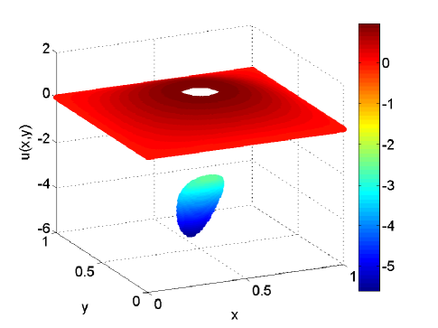
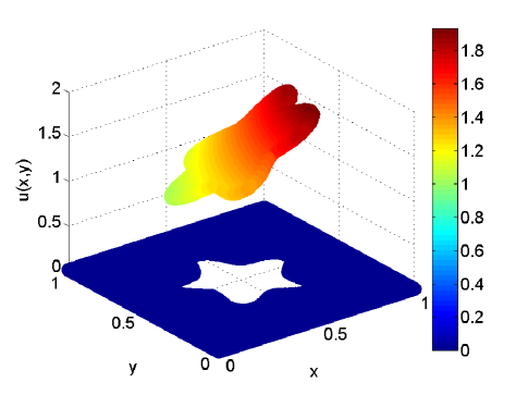
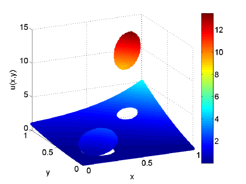
6.2 Example 1.
-
1.
Problem parameters:
-
2.
Level set defining the interface: , where , , and .
-
3.
Exact solution:
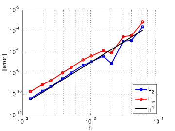
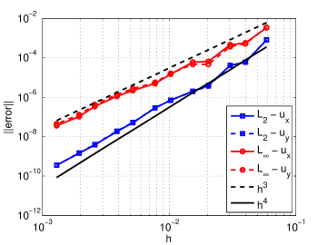
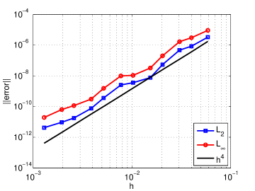
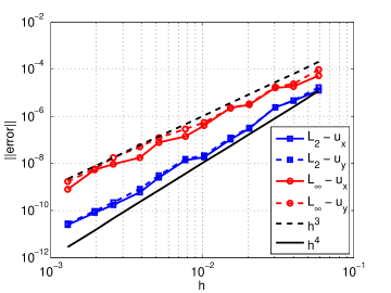
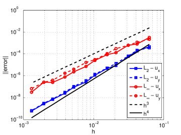
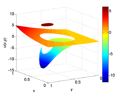
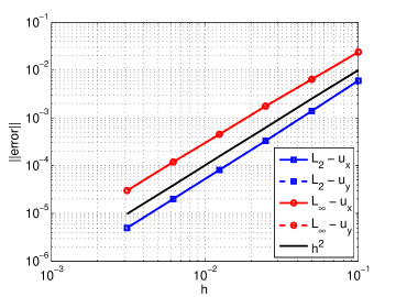
Figure 6 shows the numerical solution with a fine grid ( nodes). The discontinuity is captured very sharply, and it causes no oscillations in the solution. In addition, figure 7 shows the behavior of the error of the solution and its gradient in the and norms. As expected, the solution presents 4 order convergence as the grid is refined. Moreover, the gradient converges to 3 order in the norm and to 4 order in the norm, which is a reflection of the fact that the error in the solution is not smooth in a narrow region close to the interface only.
(a) Solution. (b) Gradient.
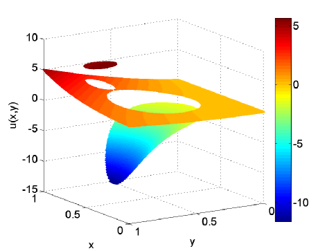
6.3 Example 2.
-
1.
Problem parameters:
-
2.
Level set defining the interface: , where , , , , , and .
-
3.
Exact solution:
Figure 8 shows the numerical solution with a fine grid ( nodes). Once again, the overall quality of the solution is very satisfactory. Figure 9 shows the behavior of the error of the solution and its gradient in the and norms. Again, the solution converges to 4 order, while the gradient converges to 3 order in the norm and close to 4 order in the norm. However, unlike what happens in example 1, small wiggles are observed in the error plots. This behavior can be explained in terms of the construction of the sets — see § 5. The approach used to construct is highly dependent on the way in which the grid points are placed relative to the interface. Thus, as the grid is refined, the arrangement of the can vary quite a lot — specially for a “complicated” interface such as the one in this example. What this means is that, while one can guarantee that the correction function is obtained with 4 order precision, the proportionality coefficient is not constant — it may vary a little from grid to grid. This variation is responsible for the small oscillations observed in the convergence plot. Nevertheless, despite these oscillations, the overall convergence is clearly 4 order.
(a) Solution. (b) Gradient.
6.4 Example 3.
-
1.
Problem parameters:
-
2.
Level set defining the interface:
, where , , , and . -
3.
Exact solution:
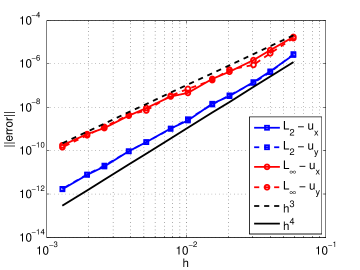
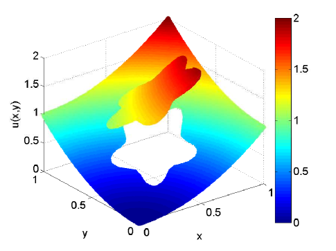
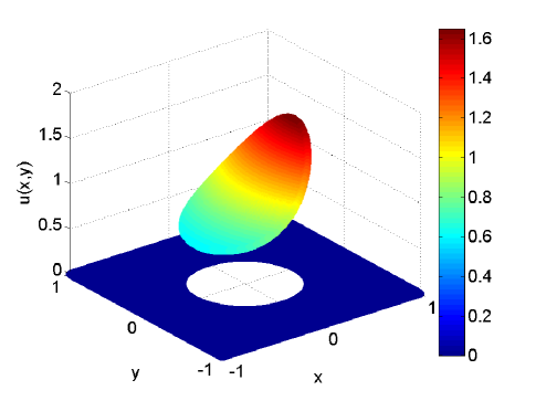
Figure 10 shows the numerical solution with a fine grid ( nodes). In this example, there are two circular interfaces in the solution domain. The two regions inside the circles make , while the remainder of the domain is . This example shows that the method is general enough to deal with multiple interfaces, keeping the same quality in the solution. Figure 11 shows that the solution converges to 4 order in both and norms, while the gradient converges to 3 order in the norm and close to 4 order in the norm.
(a) Solution. (b) Gradient.
6.5 Example 4.
-
1.
Problem parameters:
-
2.
Interface (exact representation):
-
(a)
Region 1: inside of the big circle.
-
(b)
Region 2: outer region.
-
(c)
Region 3: inside of the small circle.
-
(a)
Interface 1–2 (Big circle):
-
(b)
Interface 2–3 (Small circle):
-
(a)
-
3.
Exact solution:
Figure 12 shows the numerical solution with a fine grid ( nodes). In this example the big circle is centered within the square integration domain and the small circle is external to it, with a common point of tangency. The point of contact is placed along the boundary of the big circle at the polar angle — use the center of the big circle as the polar coordinates’ origin. These choices guarantee that, as the grid is refined, a wide variety of configurations involving two distinct interfaces crossing the same stencil occurs in a neighborhood of the contact point. In particular, the selection of the angle is so that no special alignments of the grid with the local geometry near the contact point can happen. Figure 13 shows the behavior of the error as in the and norms. Once again we observe 4 order convergence (with small superimposed oscillations) for the solution. Moreover, the gradient converges to 3 order in the norm and close to 4 order in the norm. This example shows that the CFM is robust even in situations where distinct interfaces can get arbitrarily close (tangent at a point).

(a) Solution. (b) Gradient.
6.6 Example 5.
-
1.
Problem parameters:
-
2.
Interface (exact representation):
-
(a)
Region 1: inside small circle.
-
(b)
Region 2: region between circles.
-
(c)
Region 3: outer region.
-
(a)
Interface 2–3 (Big circle):
-
(b)
Interface 1–2 (Small circle):
-
(a)
-
3.
Exact solution:
This example complements the example in § 6.5, the sole difference being that here the small circle is inside the big circle. The results are entirely similar. Figure 14 shows the numerical solution with a fine grid ( nodes), while figure 13 shows the behavior of the error in the and norms.

(a) Solution. (b) Gradient.
7 Conclusions.
In this paper we have introduced the Correction Function Method (CFM), which can, in principle, be used to obtain (arbitrary) high-order accurate solutions to constant coefficients Poisson problems with interface jump conditions. This method is based on extending the correction terms idea of the Ghost Fluid Method (GFM) to that of a correction function, defined in a (narrow) band enclosing the interface. This function is the solution of a PDE problem, which can be solved (at least in principle) to any desired order of accuracy. Furthermore, like the GFM, the CFM allows the use of standard Poisson solvers. This feature follows from the fact that the interface jump conditions modify (via the correction function) only the right-hand-side of the discretized linear system of equations used in standard linear solvers for the Poisson equation.
As an example application, the new method was used to create a 4 order accurate scheme to solve the constant coefficients Poisson equation with interface jump conditions in 2D. In this scheme, the domain of definition of the correction function is split into many grid size rectangular patches. In each patch the function is represented in terms of a bicubic (with 12 free parameters), and the solution is obtained by minimizing an appropriate (discretized) quadratic functional. The correction function is thus pre-computed, and then is used to modify (in the standard way of the GFM) the right hand side of the Poisson linear system, incorporating the jump conditions into the Poisson solver. We used the standard 4 order accurate 9-point stencil discretization of the Laplace operator, to thus obtain a 4 order accurate method.
Examples were computed, showing the developed scheme to be robust, accurate, and able to capture discontinuities sharply, without creating spurious oscillations. Furthermore, the scheme is cost effective. First, because it allows the use of standard “black-box” Poisson solvers, which are normally tuned to be extremely efficient. Second, because the additional costs of solving for the correction function scale linearly with the mesh spacing, which means that they become relatively small for large systems.
Finally, we point out that the present method cannot be applied to all the interesting situations where a Poisson problem must be solved with jump discontinuities across an interface. Let us begin by displaying a very general Poisson problem with jump discontinuities at an interface. Specifically, consider
| (23a) | ||||||
| (23b) | ||||||
| (23c) | ||||||
| (23d) | ||||||
| (23e) | ||||||
where we use the notation in § 2 and
-
7.1
The brackets indicate jumps across the interface, for example:
for . -
7.2
The subscript indicates the derivative in the direction of , the unit normal to the interface pointing towards .
-
7.3
and are smooth functions of , defined in the union of and some finite width band enclosing the interface .
-
7.4
and are smooth functions of , defined in the union of and some finite width band enclosing the interface .
-
7.5
, , and are smooth functions, defined on some finite width band enclosing the interface .
-
7.6
The Dirichlet boundary conditions in (23e) could be replaced any other standard set of boundary conditions on .
-
7.7
As usual, the degree of smoothness of the various data functions involved determines how high an order an algorithm can be obtained.
Assume now that , — where is a constant, and that
| (24) |
applies in the band enclosing where all the functions are defined.555Note that (24) implies that is a multiple of . In this case the methods introduced in this paper can be used to deal with the problem in (23) with minimal alterations. The main ideas carry through, as follows
-
7.a
We assume that both and can be extended across , so that they are defined in some band enclosing the interface.
-
7.b
We define the correction function, in the band enclosing where the and the exist, by .
-
7.c
We notice that the correction function satisfies the elliptic Cauchy problem
(25) with and at the interface .
-
7.d
We notice that the GFM correction terms can be written with knowledge of .
Unfortunately, the conditions in (24) exclude some interesting physical phenomena. In particular, in two-phase flows the case where and are constants (but distinct) and arises. We are currently investigating ways to circumvent these limitations, so as to extend our method to problems involving a wider range of physical phenomena.
Appendix A Bicubic interpolation.
Bicubic interpolation is similar to bilinear interpolation, and can also be used to represent a function in a rectangular domain. However, whereas bilinear interpolation requires one piece of information per vertex of the rectangular domain, bicubic interpolation requires 4 pieces of information: function value, function gradient, and first mixed derivative (i.e. ). For completeness, the relevant formulas for bicubic interpolation are presented below.
We use the classical multi-index notation, as in Ref. [28]. Thus, we represent the 4 vertices of the domain using the vector index . Namely, the 4 vertices are , where are the coordinates of the left-bottom vertex and is the length of the domain in the direction. Furthermore, given a scalar function , the 4 pieces of information needed per vertex are given by
| (26) |
where both and
| (27) |
Then the 16 polynomials that constitute the standard basis for the bicubic interpolation can be written in the compact form
| (28) |
where , and is the cubic polynomial
| (29) |
where and .
Finally, the bicubic interpolation of a scalar function is given by the following linear combination of the basis functions:
| (30) |
As defined above (standard bicubic interpolation), 16 parameters are needed to determine the bicubic. However, in Ref. [28] a method (“cell-based approach”) is introduced, that reduces the number of degrees of freedom to 12, without compromising accuracy. This method uses information from the first derivatives to obtain approximate formulae for the mixed derivatives. In the present work, we adopt this cell-based approach.
Appendix B Issues affecting the construction of .
B.1 Overview.
As discussed in § 5, the CFM is based on local solutions to the PDE (9) in sub-regions of – which we call . However, there is a certain degree of arbitrariness in how is defined. Here we discuss several factors that must be consider when solving equation (9), and how they influence the choice of . We also present four distinct approaches to constructing , of increasing level of robustness (and, unfortunately, complexity).
The only requirements on that the discussion in § 4 imposes are
- 1.
-
2.
should contain all the nodes where the correction function is needed.
In addition, practical algorithmic considerations further restrict the definition of , as explained below.
First, we solve for in a weak fashion, by locally minimizing a discrete version of the functional defined in equation (17). This procedure involves integrations over . Thus, it is useful if has an elementary geometrical shape, so that simple quadrature rules can be applied to evaluate the integrals. Second, if is a rectangle, we can use a (high-order) bicubic (see appendix A) to represent in . Hence we restrict to be a rectangle666Clearly, other simple geometrical shapes, with other types approximations for , should be possible — though we have not investigated them.. Third, another consideration when constructing is how the interface is represented. In principle the solution to the PDE in (9) depends on the information given along the interface only, and it is independent of the underlying grid. Nevertheless, consider an interface described implicitly by a level set function, known only in terms of its values (and perhaps derivatives) at the grid points. It is then convenient if the portions of the interface contained within can be easily described in terms of the level set function discretization — e.g. in terms of a pre-determined set of grid cells, such as the cells that define the discretization stencil. The approaches in § B.2 through § B.4 are based on this premise.
Although the prior paragraph’s strategy makes for an easier implementation, it also ties to the underlying grid, whereas it should depend only on the interface geometry. Hence it results in definitions for that cannot track the interface optimally. For this reason, we developed the approach in § B.5, which allows to freely adapt to the local interface geometry, regardless of the underlying grid. The idea is to first identify a piece of the interface based on a pre-determined set of grid cells, and then use this information to construct an optimal . This yields a somewhat intricate, but very robust definition for .
Finally, note that explicit representations of the interface are not constrained by the underlying grid. Moreover, information on the interface geometry is readily available anywhere along the interface. Hence, in this case, an optimal can be constructed without the need to identify a piece of the interface in terms of a pre-determined set of grid cells. This fact makes the approach § B.5 straightforward with explicit representations of the interface. By contrast, the less robust approaches in § B.2 through § B.4 become more involved in this context, because they requires the additional work of constraining the explicit representation to the underlying grid.
B.2 Naive Grid–Aligned Stencil–Centered Approach.
In this approach, we fit to the underlying grid by defining it as the box that covers the 9-point stencil. Figure B.1 shows two examples.
(a) Well–posed. (b) Ill–posed.
This approach is very appealing because of its simplicity, but it has serious flaws and we do not recommend it. The reason is that the piece of the interface contained within can become arbitrarily small – see figure B.1(b). Then the arguments that make the local Cauchy problem well posed no longer apply — see remarks 5, 6, and 8. In essence, the biggest frequency encoded in the interface, , can become arbitrarily large — while the characteristic length of remains . As a consequence, the condition number for the local Cauchy problem can become arbitrarily large. We describe this approach here merely as an example of the problems that can arise from too simplistic a definition of .
B.3 Compact Grid–Aligned Stencil–Centered Approach.
This is the approach described in detail in § 5.3. In summary: is defined as the smallest rectangle that
-
1.
Is aligned with the grid.
-
2.
Includes the piece of the interface contained within the stencil.
-
3.
Includes all the nodes where is needed.
Figure B.2 shows three examples of this definition. As it should be clear from this figure, a key consequence of (i–iii) is that the piece of interface contained within is always close to its diagonal — hence it is never too small relative to the size of . Consequently, this approach is considerably more robust than the one in § B.2. In fact, we successfully employed it for all the examples using the 4 order accurate scheme — see § 6.
(a) Well balanced.
(b) Well balanced.
(c) Elongated.
Unfortunately, the requirements (i–ii) in this approach tie to the grid and the stencil. As mentioned earlier, these constraints may lead to an which is not the best fit to the geometry of the interface. Figure B.2(c) depicts a situation where this strategy yields relatively poor results. This happens when there is an almost perfect alignment of the interface with the grid, which can result in an excessively elongated — in the worse case scenario, this set could reduce to a line. Although the local Cauchy problem remains well conditioned, the elongated sets can interfere with the process we use to solve the equation for in (9). Essentially, the representation of a function by a bicubic (or a modified bilinear in the case of the 2 accurate scheme in appendix C) becomes an ill-defined problem as the aspect ratio of the rectangle vanishes (however, see the next paragraph). In the authors’ experience, when this sort of alignment happens the solution remains valid and the errors are still relatively small — but the convergence rate may be affected if the bad alignment persists over several grid refinements.
We note that we observed the difficulties described in the paragraph above with the 2 accurate scheme in appendix C only. We attribute this to the fact that the bicubics result in a much better enforcement of the PDE (9) than the modified bilinears. The latter are mostly determined by the interface conditions — see remark C.1. Hence, the PDE (9) provides a much stronger control over the bicubic parameters, making this interpolation more robust in elongated sets.
Note that this issue is much less severe than the problem affecting the approach in § B.2, and could be corrected by making the Cauchy solver “smarter” when dealing with elongated sets. Instead we adopted the simpler solution of having a definition for that avoids elongated sets. The most robust way to do this is to abandon the requirements in (i–ii), and allow to adapt to the local geometry of the interface. This is the approach introduced in § B.5. A simpler, compromise solution, is presented in § B.4.
B.4 Free Stencil–Centered Approach.
Here we present a compromise solution for avoiding elongated , which abandons the requirement in (i), but not in (ii) — since (ii) is convenient when the interface is represented implicitly. In this approach is defined as the smallest rectangle that
-
1.
Is aligned with the grid rotated by an angle , where and characterizes the interface alignment with respect to the grid (e.g. the polar angle for the tangent vector to the interface section at its mid-point inside the stencil).
-
2.
Includes the piece of the interface contained within the stencil.
-
3.
Includes all the nodes where is needed.
Figure B.2 shows two examples of this approach.
(a) (b)
The implementation of the present approach is very similar to that of the one in § B.3. The only additional work is to compute and to write the interface and points where is needed in the rotated frame of reference. In both these approaches the diagonal of is very close to the piece of interface contained within the stencil, which guarantees a well conditioned local problem. However, here the addition of a rotation keeps nearly square, and avoids elongated geometries. The price paid for this is that the sets created using § B.4 can be a little larger than the ones from § B.3 — with both sets including the exact same piece of interface. In such situations, the present approach results in a somewhat larger condition number.
B.5 Node-Centered Approach.
Here we define in a fashion that is completely independent from the underlying grid and stencils. In fact, instead of associating each to a particular stencil, we define a different for each node where the correction is needed — hence the name node-centered, rather than stencil-centered. As a consequence, whereas the prior strategies lead to multiple values of at the same node (one value per stencil, see remark 10), here there is a unique value of at each node.
In this approach, is defined by the following steps:
-
1.
Identify the interface in the 4 grid cells that surround a given node. This step can be skipped if the interface is represented explicitly.
-
2.
Find the point, , along the interface that is closest to the node. This point becomes the center of . There is no need to obtain very accurately. Small errors in result in small shifts in only.
-
3.
Compute , the vector tangent to the interface at . This vector defines one of the diagonals of . The normal vector defines the other diagonal. Again, high accuracy is not needed.
-
4.
Then is the square with side length , centered at , and diagonals parallel to and — need not be aligned with the grid.
Figure B.4 shows two examples of this approach.
(a) (b)
Note that the piece of interface contained within , as defined by steps 1–4 above, is not necessarily the same found in step 1. Hence, after defining , we still need to identify the piece of interface that lies within it. For an explicit representation of the interface, this additional step is not particularly costly, but the same is not true for an implicit representation.
This approach is very robust because it always creates a square , with the interface within it close to one of the diagonals — as guaranteed by steps 2 and 3. Hence, the local Cauchy problem is always well conditioned. Furthermore, making square (to avoid elongation) does not result in larger condition numbers as in § B.4 because the larger contain an equally larger piece of the interface.
Finally, we point out that the (small) oscillations observed in the convergence plots shown in § 6 occur because in these calculations we use the approach in § B.3 — which produces sets that are not uniform in size, nor shape, along the interface. Tests we have done show that these oscillations do not occur with the node-centered approach here, for which all the are squares of the same size. Unfortunately, as pointed out earlier, the node-centered approach is not well suited for calculations using an interface represented implicitly.
Appendix C 2 Order Accurate Scheme in 2D.
C.1 Overview.
In § 5 we present a 4 order accurate scheme to solve the 2D Poisson problem with interface jump conditions, based on the correction function defined in § 4. However, there are many situations in which a 2 order version of the method could be of practical relevance. Hence, in this section we use the general framework provided by the correction function method (CFM) to develop a specific example of a 2 order accurate scheme in 2D. The basic approach is analogous to the 4 version presented in § 5. A few key points are
- 1.
-
2.
We approximate using modified bilinear interpolants (defined in § C.2), each valid in a small neighborhood of the interface. This guarantees local 2 order accuracy with only 5 interpolation parameters. Each corresponds to a grid point at which the standard discretization of Poisson’s equation involves a stencil that straddles the interface .
-
3.
The domains are rectangular regions, each enclosing a portion of , and all the nodes where is needed to complete the discretization of Poisson’s equation at the ()-th stencil. Each is a sub-domain of .
-
4.
Starting from (b) and (c), we design a local solver that provides an approximation to inside each domain .
-
5.
The interface is represented using the standard level set approach — see [27]. This guarantees a local 2 order representation of the interface, as required to keep the overall accuracy of the scheme.
-
6.
In each , we solve the PDE in (9) in a least squares sense — see remark 9. Namely, we seek the minimum of the positive quadratic integral quantity in (17), which vanishes at the solution: We substitute the modified bilinear approximation for into , discretize the integrals using Gaussian quadratures, and minimize the resulting discrete .
Remark C.1.
Using standard bilinear interpolants to approximate in each also yields 2 order accuracy. However, the Laplacian of a standard bilinear interpolant vanishes. Thus, this basis cannot take full advantage of the fact that is the solution to the Cauchy problem in (9). The modified bilinears, on the other hand, incorporate the average of the Laplacian into the formulation — see § C.2. In § C.6 we include results with both the standard and the modified bilinears, to demonstrate the advantages of the latter.
C.2 Modified Bilinear.
The modified bilinear interpolant used here builds on the standard bilinear polynomials. To define them, we use the multi-index notation — see appendix A and Ref. [28]. Thus, we label the 4 vertices of a rectangular cell using the vector index . Then the vertices are , where are the coordinates of the left-bottom vertex and is the length of the domain in the direction. The standard bilinear interpolation basis is then given by the 4 polynomials
| (31) |
where , and is the linear polynomial
| (32) |
The standard bilinear interpolation of a scalar function is given (in each cell) by
| (33) |
In the modified version, we add a quadratic term proportional to , so that the Laplacian of the modified bilinear is no longer identically zero. The coefficient of the quadratic term can be written in terms of the average value of the Laplacian over the domain, . This yields the following formula for the modified bilinear interpolant
| (34) |
C.3 Standard Stencil.
We use the standard 2 order accurate 5-point discretization of the Poisson equation
| (35) |
where is defined in (11). In the absence of discontinuities, (35) provides a compact 2 order accurate representation of the Poisson equation. In the vicinity of the discontinuities at the interface , we define an appropriate domain , and use it to compute the correction terms needed by (35) — as described below.
To understand how the correction terms affect the discretization, consider the situation in figure C.1. In this case, the node lies in while the nodes and are in . Hence, to be able to use equation (35), we need to compute and .
After having solved for where necessary (see § C.4 and § C.5), we modify equation (35) and write
| (36) |
which differs from (35) by the terms on the RHS only. Here the are the CFM correction terms needed to complete the stencil across the discontinuity at . In the particular case illustrated by figure C.1, we have
| (37) |
Similar formulas apply for all the other possible arrangements of the stencil for the Poisson’s equation, relative to the interface .
C.4 Definition of .
As discussed in appendix B, the construction of presented in § 5.3 may lead to elongated shapes for , which can cause accuracy loses. As mentioned earlier (see the end of § B.3) this is not a problem for the 4 order scheme, but it can be one for the 2 order one. To resolve this issue we could have implemented the robust construction of given in § B.5. However the simpler compromise version in § B.4 proved sufficient.
The approach in § B.4 requires to include the piece of interface contained “within the stencil.” For the 9-point stencil, this naturally means “within the box aligned with the grid that includes the nine points of the stencil.” We could use the same meaning for the 5-point stencil, but this would not take full advantage of the 5-point stencil compactness. A better choice is to use the quadrilateral defined by the stencil’s four extreme points — i.e. the dashed box in figure C.1. This choice is used only to determine the piece of interface to be included within . It does not affect the definition of the interface alignment angle used by the § B.4 approach. Hence the following four steps define
-
1.
Find the angle between the vector tangent to the interface at the mid-point within the stencil, and the -axis. Introduce the coordinate system -, resulting from rotating - by — see figure C.2(a).
-
2.
Find the coordinates and characterizing the smallest - coordinate rectangle enclosing the section of the interface contained within the stencil — see figure C.2(b).
-
3.
Find the coordinates and characterizing the smallest - coordinate rectangle enclosing all the nodes at which is needed — see figure C.2(b).
-
4.
is the smallest - coordinate rectangle enclosing the two previous rectangles. Its edges are characterized by
(38a) (38b) (38c) (38d)
Figure C.2 shows an example of defined in this way.
(a) Step 1. (b) Steps 2–4.
C.5 Solution of the Local Cauchy Problem.
The remainder of the 2 order accurate scheme follows the exact same procedure used for the 4 order accurate version described in detail in § 5. In particular, as explained in item (f) of § C.1, we solve the local Cauchy problem defined by equation (9) in a least squares sense (using the same minimization procedure described in § 5.4). The only differences are that: (i) In the 2 order accurate version of the method we use 4 Gaussian quadrature points for the 1D line integrals, and 16 points for the 2D area integrals. (ii) Because the modified bilinear representation for involves 5 basis polynomials, the minimization problem produces a (self-adjoint) linear system — instead of the system that occurs for the 4order algorithm.
C.6 Results
Here we present three examples of solutions to the 2D Poisson’s equation using the algorithm described above. Each example is defined below in terms of the problem parameters (source term and jump conditions across the interface ), the representation of the interface, and the exact solution (needed to evaluate the errors in the convergence plots). Note that
-
1.
In all cases we represent the interface using a level set function .
-
2.
Below the level set function is described via an analytic formula. This formula is converted into a discrete level set representation used by the code. Only this discrete representation is used for the actual computations.
-
3.
The level set formulation allows us to compute the vectors normal to the interface to 2 order accuracy with a combination of finite differences and standard bilinear interpolation. Hence, it is convenient to write the jump in the normal derivative, , in terms of the jump in the gradient of dotted with the normal to the interface .
We use777A subscript s is added to the example numbers of the 2order method, to avoid confusion with the 4order method examples. example 1s to test the 2 order scheme in a generic problem with a non-trivial interface geometry. In addition, in this example the correction function has a non-zero Laplacian. Thus, we used this problem to compare the performance of the Standard Bilinear (SB) and Modified Bilinear (MB) interpolations as basis for the correction function. Finally, examples 2s and 3s here correspond to examples 1 and 3 in [3], respectively. Hence they can be used to compare the performance of the present 2 order scheme with the Immersed Interface Method (IIM), in two distinct situations.
C.6.1 Example 1s.
-
1.
Domain: .
-
2.
Problem parameters:
-
3.
Level set defining the interface: ,
where , , , , , and . -
4.
Exact solution:
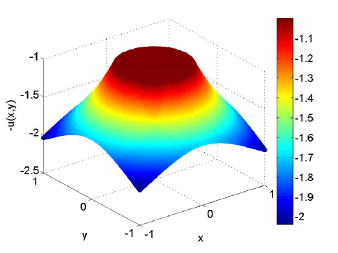
Figure C.3 shows the numerical solution with a fine grid ( nodes). The non-trivial contour of the interface is accurately represented and the discontinuity is captured very sharply. For comparison we solved this problem using both the SB and MB interpolations to represent the correction function. Although figure C.3 shows the solution obtained with the modified bilinear version, both versions produce small errors and are visually indistinguishable.
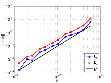
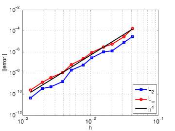
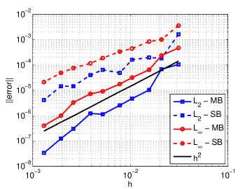
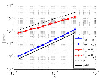
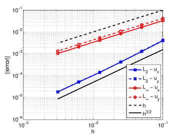
Figure C.4(a) shows the convergence of the solution error in the and norms, for both the SB and MB versions. As expected, the overall behavior indicates 2 order convergence, despite the small oscillations that are characteristic of this implementation of the method, as explained in § 6.3. Note that the MB version produces significantly smaller errors (a factor of about 20) than the SB version. It also exhibits a more robustly 2 order convergence rate. Moreover, figure C.4(b) shows the convergence of the error of the gradient of the MB solution in the and norms. Here, the gradient was computed using standard 2 order accurate centered differences, as in (21) and (22). As we can observe, the gradient converges to 1 order in the norm and, apparently, as in the norm.
(a) Solution. (b) Gradient.
C.6.2 Example 2s.
-
1.
Domain: .
-
2.
Problem parameters:
-
3.
Level set defining the interface: ,
where , , and . -
4.
Exact solution:
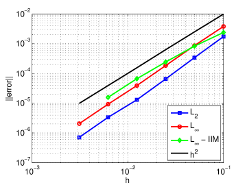
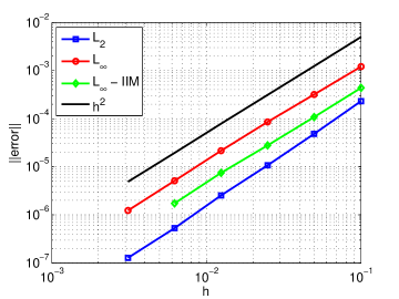
As mentioned earlier, this example corresponds to example 1 in [3], where the same problem is solved using the Immersed Interface Method. Hence, this provides a good opportunity to compare the CFM with the well established IIM. Figure C.5 shows the numerical solution with a fine grid ( nodes). Once again, the overall quality of the solution is very satisfactory. Figure C.6 shows the behavior of the error in the and norms and the solution converges to 2 order. However, in this example the gradient also appears to converge to 2 order.
Figure C.6(a) also includes the convergence of the solution error in the norm obtained with the IIM — we plot the errors listed in table 1 of [3]. Both methods produce similar convergence rates. However, in this example at least, the CFM produces slightly smaller errors — by a factor of about 1.7.
(a) Solution. (b) Gradient.
C.6.3 Example 3s.
-
1.
Domain: .
-
2.
Problem parameters:
-
3.
Level set defining the interface: ,
where , , and . -
4.
Exact solution:
This example corresponds to example 3 in [3] for the IIM method. Figure C.7 shows the numerical solution with a fine grid ( nodes) while figure C.8 presents convergence results for the errors in the and norms. In addition, figure C.8(a) also includes the norm of the error obtained with the IIM — we plot the errors listed in table 3 of [3]††footnotemark: . In this case the IIM produces slightly smaller errors than the CFM — by a factor of about 2.8. Therefore, based on the results from examples 2s and 3s, we may conclude that the IIM and the CFM produce results of comparable accuracy — each method generating slightly smaller errors in different cases.
(a) Solution. (b) Gradient.
Acknowledgements
The authors would like to acknowledge the National Science Foundation support — this research was partially supported by grant DMS-0813648. In addition, the first author acknowledges the support by Coordenação de Aperfeiçoamento de Pessoal de Nível Superior (CAPES – Brazil) and the Fulbright Commission through grant BEX 2784/06-8. The second author also acknowledges support from the NSERC Discovery program. Finally, the authors would also like to acknowledge many helpful conversations with Prof. B. Seibold at Temple University, and the many helpful suggestions made by the referees of this paper.
References
References
- [1] C. S. Peskin, Numerical analysis of blood flow in the heart, Journal of Computational Physics 25 (3) (1977) 220–252. doi:10.1016/0021-9991(77)90100-0.
- [2] M. Sussman, P. Smereka, S. Osher, A level set approach for computing solutions to incompressible two-phase flow, Journal of Computational Physics 114 (1) (1994) 146–159. doi:10.1006/jcph.1994.1155.
- [3] R. J. LeVeque, Z. Li, The immersed interface method for elliptic equations with discontinuous coefficients and singular sources, SIAM Journal on Numerical Analysis 31 (4) (1994) 1019–1044. doi:10.1137/0731054.
- [4] R. J. LeVeque, Z. Li, Immersed interface methods for Stokes flow with elastic boundaries or surface tension, SIAM Journal on Scientific Computing 18 (3) (1997) 709–735. doi:10.1137/S1064827595282532.
- [5] H. Johansen, P. Colella, A Cartesian grid embedded boundary method for Poisson’s equation on irregular domains, Journal of Computational Physics 147 (1) (1998) 60–85. doi:10.1006/jcph.1998.5965.
- [6] R. P. Fedkiw, T. Aslam, S. Xu, The ghost fluid method for deflagration and detonation discontinuities, Journal of Computational Physics 154 (2) (1999) 393–427. doi:10.1006/jcph.1999.6320.
- [7] R. P. Fedkiw, T. Aslam, B. Merriman, S. Osher, A non-oscillatory Eulerian approach to interfaces in multimaterial flows (the ghost fluid method), Journal of Computational Physics 152 (2) (1999) 457–492. doi:10.1006/jcph.1999.6236.
- [8] M. Kang, R. P. Fedkiw, X.-D. Liu, A boundary condition capturing method for multiphase incompressible flow, Journal of Scientific Computing 15 (2000) 323–360. doi:10.1023/A:1011178417620.
- [9] X.-D. Liu, R. P. Fedkiw, M. Kang, A boundary condition capturing method for Poisson’s equation on irregular domains, Journal of Computational Physics 160 (1) (2000) 151–178. doi:10.1006/jcph.2000.6444.
- [10] M.-C. Lai, C. S. Peskin, An immersed boundary method with formal second-order accuracy and reduced numerical viscosity, Journal of Computational Physics 160 (2) (2000) 705–719. doi:10.1006/jcph.2000.6483.
- [11] Z. Li, M.-C. Lai, The immersed interface method for the Navier-Stokes equations with singular forces, Journal of Computational Physics 171 (2) (2001) 822–842. doi:10.1006/jcph.2001.6813.
- [12] D. Q. Nguyen, R. P. Fedkiw, M. Kang, A boundary condition capturing method for incompressible flame discontinuities, Journal of Computational Physics 172 (1) (2001) 71–98. doi:10.1006/jcph.2001.6812.
- [13] L. Lee, R. J. LeVeque, An immersed interface method for incompressible Navier-Stokes equations, SIAM Journal on Scientific Computing 25 (3) (2003) 832–856. doi:10.1137/S1064827502414060.
- [14] F. Gibou, L. Chen, D. Nguyen, S. Banerjee, A level set based sharp interface method for the multiphase incompressible Navier-Stokes equations with phase change, Journal of Computational Physics 222 (2) (2007) 536–555. doi:10.1016/j.jcp.2006.07.035.
- [15] Y. Gong, B. Li, Z. Li, Immersed–interface finite-element methods for elliptic interface problems with nonhomogeneous jump conditions, SIAM Journal on Numerical Analysis 46 (1) (2008) 472–495. doi:10.1137/060666482.
- [16] J. Dolbow, I. Harari, An efficient finite element method for embedded interface problems, International Journal for Numerical Methods in Engineering 78 (2) (2009) 229–252. doi:10.1002/nme.2486.
- [17] J. Bedrossian, J. H. von Brecht, S. Zhu, E. Sifakis, J. M. Teran, A second order virtual node method for elliptic problems with interfaces and irregular domains, Journal of Computational Physics 229 (18) (2010) 6405 – 6426. doi:DOI:10.1016/j.jcp.2010.05.002.
- [18] L. N. Trefethen, D. Bau, Numerical Linear Algebra, SIAM: Society for Industrial and Applied Mathematics, 1997.
- [19] A. Mayo, The fast solution of Poisson’s and the biharmonic equations on irregular regions, SIAM Journal on Numerical Analysis 21 (2) (1984) 285–299. doi:10.1137/0721021.
- [20] H. S. Udaykumar, R. Mittal, W. Shyy, Computation of solid-liquid phase fronts in the sharp interface limit on fixed grids, Journal of Computational Physics 153 (2) (1999) 535–574. doi:10.1006/jcph.1999.6294.
- [21] F. Gibou, R. P. Fedkiw, L.-T. Cheng, M. Kang, A second-order-accurate symmetric discretization of the Poisson equation on irregular domains, Journal of Computational Physics 176 (1) (2002) 205–227. doi:10.1006/jcph.2001.6977.
- [22] Z. Jomaa, C. Macaskill, The embedded finite difference method for the Poisson equation in a domain with an irregular boundary and Dirichlet boundary conditions, Journal of Computational Physics 202 (2) (2005) 488–506. doi:10.1016/j.jcp.2004.07.011.
- [23] F. Gibou, R. Fedkiw, A fourth order accurate discretization for the Laplace and heat equations on arbitrary domains, with applications to the Stefan problem, Journal of Computational Physics 202 (2) (2005) 577–601. doi:10.1016/j.jcp.2004.07.018.
- [24] H. Chen, C. Min, F. Gibou, A supra-convergent finite difference scheme for the Poisson and heat equations on irregular domains and non-graded adaptive Cartesian grids, Journal of Scientific Computing 31 (1) (2007) 19–60. doi:10.1007/s10915-006-9122-8.
- [25] J. A. Sethian, J. Strain, Crystal growth and dendritic solidification, Journal of Computational Physics 98 (2) (1992) 231–253. doi:10.1016/0021-9991(92)90140-T.
- [26] S. Chen, B. Merriman, S. Osher, P. Smereka, A simple level set method for solving Stefan problems, Journal of Computational Physics 135 (1) (1997) 8–29. doi:10.1006/jcph.1997.5721.
- [27] S. Osher, J. A. Sethian, Fronts propagating with curvature–dependent speed: Algorithms based on hamilton-jacobi formulations, Journal of Computational Physics 79 (1) (1988) 12 – 49. doi:DOI:10.1016/0021-9991(88)90002-2.
- [28] J.-C. Nave, R. R. Rosales, B. Seibold, A gradient-augmented level set method with an optimally local, coherent advection scheme, Journal of Computational Physics 229 (10) (2010) 3802 – 3827. doi:10.1016/j.jcp.2010.01.029.