AGN Driven Weather and Multiphase Gas in the Core of the NGC 5044 Galaxy Group

Abstract

A deep Chandra observation of the X-ray bright group, NGC 5044, shows that the central region of this group has been strongly perturbed by repeated AGN outbursts. These recent AGN outbursts have produced many small X-ray cavities, cool filaments and cold fronts. We find a correlation between the coolest X-ray emitting gas and the morphology of the H$\alpha$ filaments. The H$\alpha$ filaments are oriented in the direction of the X-ray cavities, suggesting that the warm gas responsible for the H$\alpha$ emission originated near the center of NGC 5044 and was dredged up behind the buoyant, AGN-inflated X-ray cavities. A detailed spectroscopic analysis shows that the central region of NGC 5044 contains spatially varying amounts of multiphase gas. The regions with the most inhomogeneous gas temperature distribution tend to correlate with the extended 235 MHz and 610 MHz radio emission detected by the GMRT. This may result from gas entrainment within the radio emitting plasma or mixing of different temperature gas in the regions surrounding the radio emitting plasma by AGN induced turbulence. Accounting for the effects of multiphase gas, we find that the abundance of heavy elements is fairly uniform within the central 100 kpc, with abundances of 60-80% solar for all elements except oxygen, which has a significantly sub-solar abundance. In the absence of continued AGN outbursts, the gas in the center of NGC 5044 should attain a more homogeneous distribution of gas temperature through the dissipation of turbulent kinetic energy and heat conduction in approximately $10^{8}$ yr. The presence of multiphase gas in NGC 5044 indicates that the time between recent AGN outbursts has been less than $\sim 10^{8}$ yr.

1 Introduction

Chandra and XMM-Newton observations have shown that there is a strong feedback mechanism between the central AGN and the energetics of the hot gas in groups and clusters of galaxies (e.g., Peterson & Fabian 2006 and McNamara & Nulsen 2007). AGN outbursts in the central dominant galaxy in groups and clusters, which are themselves fueled by the accretion of cooling gas, can produce shocks, buoyant cavities and sound waves, all of which lead to re-heating of the cooling gas. This AGN-cooling flow feedback mechanism is also an important process in galaxy formation and can explain the observed correlation between bulge mass and central black hole mass (e.g., Gebhardt et al. 2000) and the cut-off in the number of massive galaxies (Croton et al. 2006).

AGN outbursts can have a much more significant impact on the energetics of the hot gas in groups compared to that in richer clusters, due to their shallower potential wells. In David et al. (2009), hereafter Paper I, we presented the results of an 80 ksec Chandra observation of the X-ray bright group, NGC 5044, and showed that the central region of this group has been perturbed by several recent AGN outbursts and also by motion of the central galaxy relative to the surrounding intragroup gas. GMRT observations at 235 MHz and 610 MHz show direct evidence for uplifting of low entropy gas from the center of NGC 5044 behind buoyant, AGN-inflated X-ray cavities. Most of the X-ray cavities in NGC 5044, however, remain radio quiet in our GMRT observations. The roughly isotropic distribution of the small radio quiet cavities suggests that the group weather has a significant impact on the dynamics of these bubbles as they buoyantly rise. We also showed in Paper I that the total mechanical power of the small radio quiet cavities is sufficient to suppress about one-half of the total radiative cooling within the central 10 kpc. In this paper, we discuss how AGN driven turbulence has produced a multiphase medium in the center of NGC 5044 and how and this impacts estimates of the abundance and distribution of heavy elements.

This paper is organized in the following manner. Details of the ACIS data analysis are described in $\S 2$. Section 3 presents temperature and abundance maps for the center of NGC 5044 and $\S 4$ contains a discussion about systematic effects in the derivation of elemental abundances when fitting emission from multiphase gas with non-solar abundance ratios. In $\S 5$ we show how abundance profiles for NGC 5044 depend on the assumed spectral model. Section 6 presents a comparison between XMM-Newton and Chandra derived abundances. Correlations between the X-ray and H $/alpha$ emission are discussed in $\S 7$. The implications of our results are discussed in $\S 8$ and $\S 9$ contains a brief summary of our main results.

2 Data Analysis

NGC 5044 was observed by Chandra on March 7, 2008 (ObsId 9399) for a total of 82710 sec. All data analysis was performed with CIAO 4.2 and CALDB 4.2.1. Since the X-ray emission from NGC 5044 completely fills the S3 chip, the back-side illuminated chip S1 was used to screen for background flares. Light curves were made in the 2.5-7.0 keV and 9.0-12.0 keV energy bands for the diffuse emission on S1. No background flares exceeding a count rate threshold of 20% above the quiescent background count rate were detected during the observation. Background images were generated from the standard set of blank sky images in the Chandra CALDB and the exposure times in the background images were adjusted to yield the same 9.0-12.0 keV count rates as in the NGC 5044 data (see Paper I for more details about the data analysis). The GMRT data for NGC 5044 was obtained as part of a low frequency radio survey of elliptical-dominated galaxy groups (see Giacintucci et al. 2010; Gitti el at. 2010). Throughout this paper we use a luminosity distance of $D_{L}=38.8$ Mpc for NGC 5044, which corresponds to $1^{\prime\prime}=185$ pc.

3 Temperature and Abundance Maps

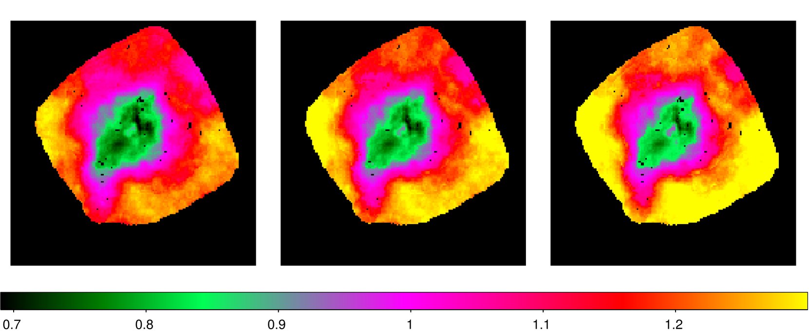
Figure 1: Temperature map covering the ACIS-S3 chip. The central panel shows the best-fit temperature and the left and right panels show the 90% lower and upper limits on the temperature. The spectra were fit with an absorbed apec model with the temperature, abundance and normalization treated as free parameters and the absorption fixed at the galactic value.

A temperature map covering the ACIS-S3 chip (approximately 90 kpc on a side) is shown in Figure 1. The temperature map was derived using the same method described in O’Sullivan et al. (2005). All spectra were fit to an absorbed apec model with the absorption fixed to the galactic value ($N_{H}(gal)=4.94\times 10^{20}$ cm^-2) and the temperature, abundance and normalization treated as free parameters. Regions were chosen to include at least 1600 net counts. The middle panel of Figure 1 shows the best-fit temperature and the left and right hand panels show the 90% lower and upper limits on the temperature. The temperature map shown in Figure 1 is very similar to the temperature map presented in Paper I, which was derived from the energy centroid of the blended Fe-L lines. Figure 1 shows that there is a great deal of structure in the temperature map and that the coolest gas extends toward the SE. As discussed in Paper I, all of the bright X-ray filaments contain cooler gas compared to the surrounding regions. A more in depth discussion of the features in the NGC 5044 temperature map is given in Paper I.

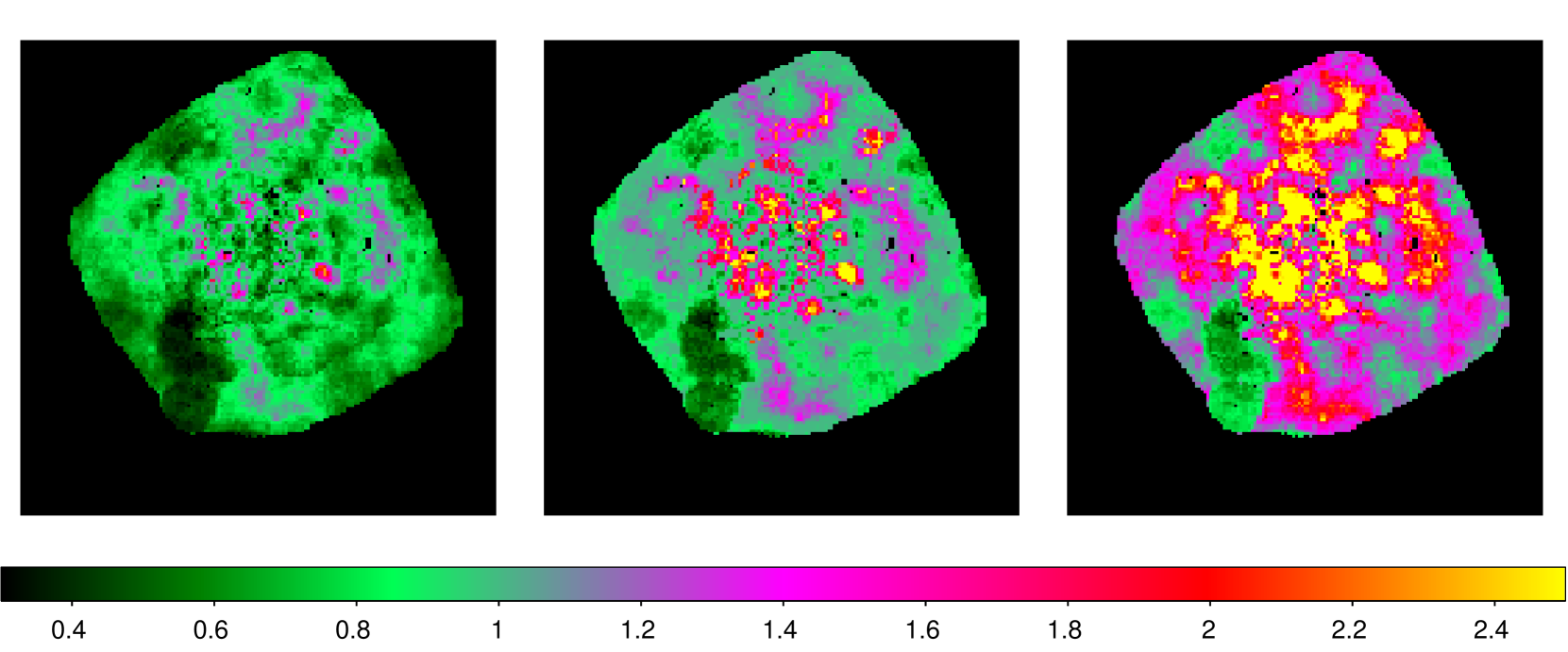
Figure 2: Abundance map covering for the ACIS-S3 chip. The central panel shows the best-fit abundance and the left and right panels show the 90% lower and upper limits on the abundance. The spectra were fit with an absorbed apec model with the temperature, abundance and normalization treated as free parameters and the absorption fixed at the galactic value.

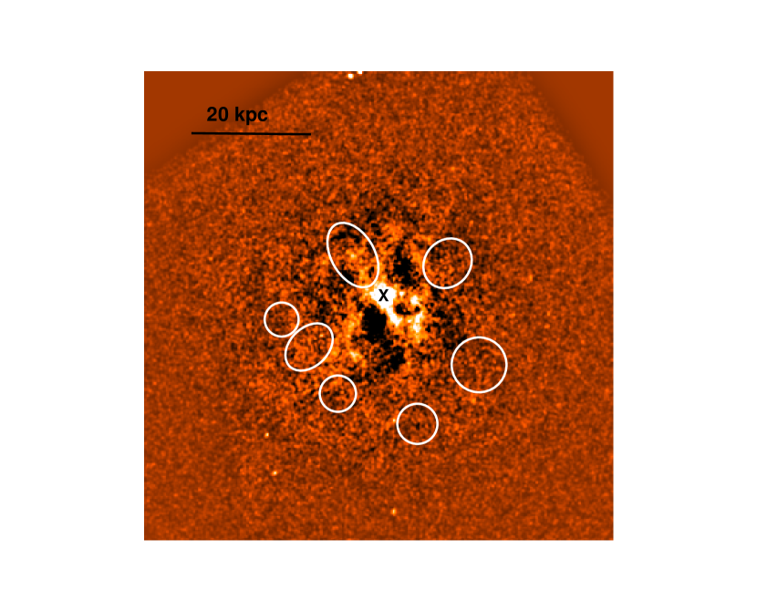
Figure 3: Location of the high abundance clouds detected in the abundance map highlighted on the unsharp masked image of NGC 5044. The ”X” marks the location of the AGN at the center of NGC 5044.

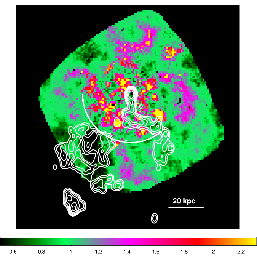
Figure 4: GMRT 235 MHz contours overlayed on the abundance map (central panel of Fig. 4). The beam size is 22^′′ by 16^′′ and the lowest contour is shown at $3\sigma=0.75$ mJy b^-1 = 0.2mJy/b. The white arc shows the location of the SE cold front (see Paper I).

The corresponding abundance map for NGC 5044 is shown in Figure 2. All 3 panels in Figure 2 show the presence of cloud-like and filament-like regions of high abundance gas. There is also a large extended region of very low abundance gas in the SE corner of the S3 chip. Most of the high abundance clouds are located at larger radii than the central X-ray cavities (see Figure 3), but interior to the SE cold front noted in Paper I (see Figure 4). The high abundance filaments are primarily located at larger radii than the SE cold front. Except for the spatial coincidence between the high abundance cloud toward the NE and an X-ray bright filament, there are no significant correlations between the high abundance regions, features in the ACIS image, the unsharp masked image, or the temperature map.

As discussed in Paper I, the 235 MHz radio emission passes through the southern X-ray cavity, bends to the west just behind the SE cold front and then undergoes another sharp bend toward the south, at the location of the SE cold front. Figure 4 shows that the 235MHz radio emission passes through regions with the lowest abundances and threads the region between the high abundance clouds. The lowest abundance gas is located in the SW corner of S3, at the same position as the detached 235 MHz radio lobe.

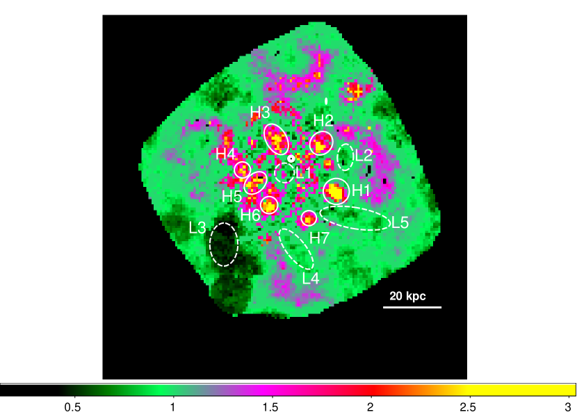
Figure 5: High and low abundance regions used for more in-depth spectral analysis. The small heavy white circle indicates the location of the AGN at the center of NGC 5044.

To determine the accuracy of the method used for deriving the abundances shown in Figure 2, we extracted spectra from 7 regions with super solar abundances and 5 regions with sub solar abundances (see Figure 5). These spectra were then fit to a single apec model in the 0.5-3.0 keV energy band with the absorption fixed at the galactic value (see the results in Table 1). These results are in good agreement with the trends seen in the abundance map and show that the abundances differ by a factor of approximately 3 between the high and low abundance regions.

4 Systematic Effects in Measuring Abundances of Heavy Elements

Care must always be taken when estimating abundances for gas which is likely multiphase (e.g., Buote et al. 1999; Rasia et al. 2008). In general, abundance estimates derived from fitting CCD resolution spectra of multiphase gas are highly model-dependent. Abundances are usually underestimated when fitting the emission from multi-phase gas with temperatures of $\sim$1 keV with single temperature models. The abundance map shown in Figure 2 is based on fitting the projected spectra to an absorbed apec model with the absorption fixed at the galactic value. In addition to the presence of multiphase gas, the derived abundances can also be affected by unresolved LMXBs, non-solar ratios of heavy elements, excess absorption and projection effects.

4.1 Unresolved LMXBs

In paper I, we found that the power-law emission from unresolved LMXBs can affect the derived spectral properties in the central region of NGC 5044. We also derived the ratio between the X-ray luminosity of the LMXBs and the K-band luminosity of NGC 5044 in Paper I. Using this ratio, and the 2MASS image of NGC 5044, we re-fit the spectra extracted from the high and low abundance regions shown in Figure 5 with an absorbed apec plus power-law model with the normalization of the power-law component frozen at the value derived from the K-band luminosity within each region. We found that the improvement in the quality of the fits is statistically insignificant (based on a F-test) and that there is no significant effect on the derived abundances. This is mainly due to the use of a soft energy band (0.5-3.0 keV) in our spectral analysis. Paper I showed that unresolved emission from LMXBs primarily affects the spectroscopic results when higher energy photons are included in the analysis.

4.2 Non-Solar Abundance Ratios

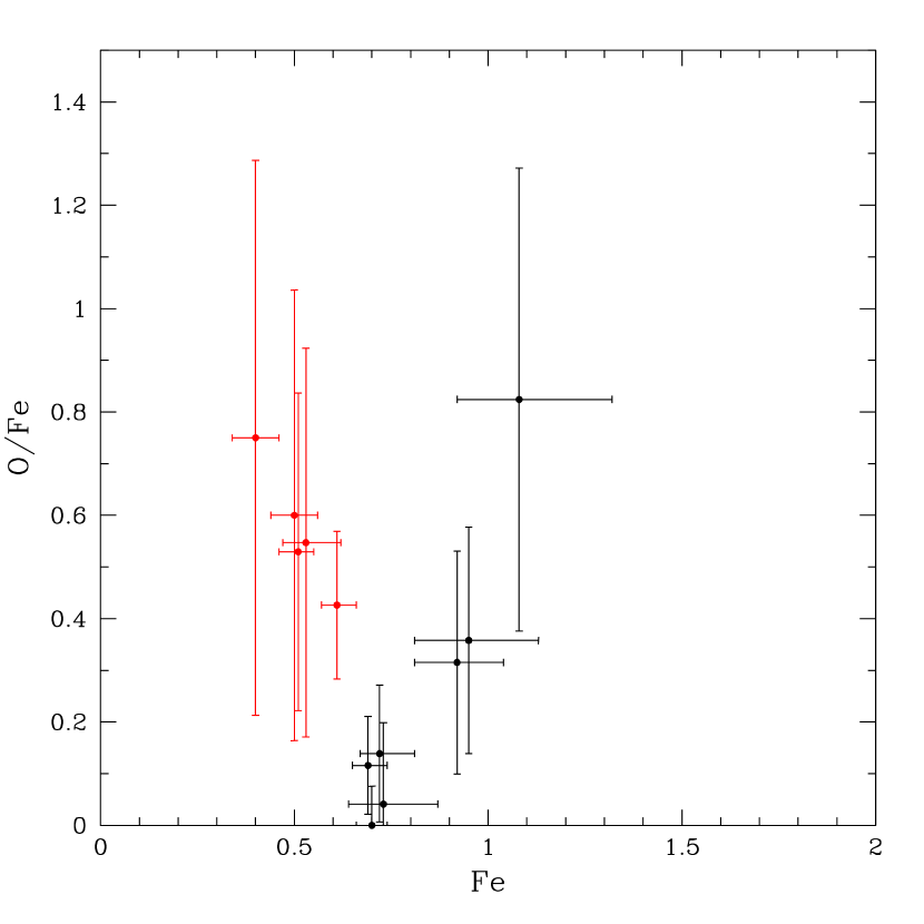
Figure 6: Scatter plot of the O/Fe ratios and Fe abundances for the high abundance clouds (black) and low abundance regions (red) derived from fitting the spectra to a single-temperature vapec model. All error bars are shown at $1\sigma$.

We next fit the set of spectra to an absorbed apec model with free absorption, an absorbed vapec model with free O, Mg, Ne, Si, S and Fe abundances (freeing up one element at a time) and an absorbed two temperature vapec model. The single greatest improvement in the quality of the spectral fits (based on a F-test) was obtained by fitting the spectra with an absorbed vapec model with the absorption fixed at the galactic value and O and Fe allowed to vary independently. The results of this spectral analysis are shown in Table 2. This table shows that for 6 of the 7 high abundance regions, there is a statistically significant improvement in the quality of the spectral fits. For the low abundance regions, the quality of the fits is only improved in 1 out of 5 regions. While the derived Fe abundances in the high abundance regions are still significantly greater than the Fe abundances in the low abundance regions (compare Tables 1 and 2), the ratio of the average Fe abundance between the high and low abundance regions is significantly reduced by allowing O and Fe to vary independently. Figure 6 shows that the high and low abundance regions also have different O/Fe ratios. The high abundance regions tend to have low O/Fe ratios, while the low abundance regions have O/Fe ratios mostly consistent with the solar ratio (which is why the low abundance regions are well fit with an apec model).

To demonstrate the dependence of the abundance, Z, derived from fitting an apec model to gas with a non-solar O/Fe ratio, we simulated a set of 1 keV spectra using a vapec model with a solar abundance of Fe and a range of O/Fe values. These spectra were then fit with an apec model. Figure 7 shows that the best-fit abundance derived from an apec model can be significantly overestimated when fitting the emission from gas with an intrinsically low O/Fe ratio. By excising the O emission in the spectral analysis, and only fitting the data in the 0.8-3.0 keV energy band, we find that the abundance derived from an apec model is consistent with the Fe abundance derived from a vapec model (see Table 3). Freeing up additional heavy elements in the vapec model (i.e., Mg, Ne, Si and S) did not produce a statistically significant improvement in the spectral analysis or alter the best-fit O and Fe abundances given in Table 2.

4.3 Excess Absorption

It is possible that the low O/Fe ratios derived in the high abundance regions are due to excess absorption which would preferentially absorb the O emission-lines. We therefore generated a set of simulated vapec spectra with solar O/Fe ratios and a range of excess absorption. These spectra were then fit to a vapec model with the O and Fe abundances treated as free parameters and the absorption fixed at the galactic value. The sensitivity of the derived O/Fe ratio as a function of excess absorption is shown in Figure 8. This figure shows that at least $5\times 10^{20}$ cm^-2 of excess absorption is required to produce the low O/Fe ratios observed in the high abundance regions. Table 4 shows the results of fitting the sample spectra to a vapec model with $N_{H}$ and the O and Fe abundances treated as free parameters. Based on a F-test, there is very little statistical improvement in the quality of the fits compared to that obtained with $N_{H}$ fixed at the galactic value. In addition, only 2 of the 12 regions have a best-fit excess $N_{H}$ of more than $1.0\times 10^{20}$ cm^-2 at the 90% confidence limit. There is also no correlation between the O/Fe ratio and the best-fit excess $N_{H}$ among these regions.

The low energy QE of the ACIS detectors has continued to decrease during the course of the Chandra mission due to out gassed material condensing on the cold ACIS filters. Our analysis uses the latest update to the ACIS contamination model which was released in CALDB 4.2 on December 15, 2009, however, systematic uncertainties in the ACIS contamination model could affect our derived O abundances. In addition to the energy dependence of the absorbing material, the ACIS-S contamination model also includes a time-dependence and a dependence on chipy (parallel to the read-out direction). To estimate the systematic uncertainty in the CALDB 4.2 version of the ACIS contamination model, we extracted a spectrum from the 2009 observation of the Coma cluster (which has a very low galactic column density of $N_{H}=8.5\times 10^{19}$) spanning the same range in chipy as that covered by the high abundance clouds in the NGC 5044 observation. The spectrum was then fit to an absorbed apec model with the absorption treated as a free parameter. We obtained a best-fit $N_{H}$ of $5.5\times 10^{19}$ with a 90% upper limit of $N_{H}=1.3\times 10^{20}$. Thus, excess absorption due to systematic uncertainties in the ACIS contamination model should be less than $4.5\times 10^{19}$ around the time of the NGC 5044 observation. Such a small systematic uncertainty cannot account for the low observed values of the O/Fe ratio (see Figure 8).

4.4 Multiphase Gas

Table 5 shows the results of fitting the spectra to a two-temperature vapec model with the O and Fe abundances linked between the two temperature components and the absorption fixed at the galactic value. For regions H1, H7 and L5, the two temperature fits were essentially degenerate with respect to the single temperature fits (i.e., the values for the two temperatures overlap within their uncertainties). For these regions, we replicate the results from the single temperature analysis in Table 5. Table 5 shows that the improvement in the quality of the spectral fits for 7 of the 9 remaining spectra is highly significant with the addition of a second temperature component. One obvious difference between the low and high abundance regions is the fraction of the total flux from the cooler component. In the high abundance regions, the cooler component accounts for approximately 80% of the total flux, while in the low abundance regions, the flux from the cool and hot components is more evenly distributed.

Due to the complexity in the abundance map, we cannot perform a simple deprojection analysis. Since we are fitting projected spectra, some of the improvement obtained by fitting a two-temperature model to the spectra probably arises from the range in gas temperatures along the line-of-sight. Using the deprojected temperature and density profiles for NGC 5044, we calculated the flux arising from gas at different temperatures. Figure 9 shows the cumulative fraction of the 0.5-3.0 keV flux, relative to the total flux, arising from gas cooler than a given temperature along three different projected distances (b=10, 20 and 30 kpc) from the center of NGC 5044. Most of the spectral extraction regions shown in Figure 5 are located approximately 20 kpc from the center of NGC 5044. Figure 9 shows that for a projected distance of b=20 kpc, approximately 20% of the emission should arise from gas hotter than 1 keV due to projection effects. This is in good agreement with the $F_{c}/F_{tot}$ ratios for the high abundance regions (see Table 5), indicating that the emission from within the high abundance regions themselves is nearly single-phased. The greater fraction of emission from hotter gas in the low abundance regions indicates that the gas within these regions has a greater predominance of multiphase gas.

The resulting O/Fe ratios and Fe abundances from a two-temperature spectral analysis are shown in Fig. 10. Fitting the spectra to two-temperature models lessens the Fe abundance contrast between the regions initially identified as having high and low abundances based on the spectral analysis with an apec model. From Table 1, the ratio of the average abundance in the high abundance regions to the average abundance in the low abundance regions is 2.5. Fitting the spectra with a vapec model with Fe and O treated as free parameters gives an average Fe abundance ratio between the high and low abundance regions of 1.6 (see Table 2). The average Fe abundance contrast between the high and low abundance regions is further reduced to 1.3, when the spectra are analyzed with a two-temperature model (see Table 5). Tables 2 and 5 show that the primary reason for the reduction in the Fe abundance contrast is a 52% increase in the Fe abundance in the low abundance regions compared to only a 26% increase in the Fe abundance in the high abundance regions, when a second temperature component is added.

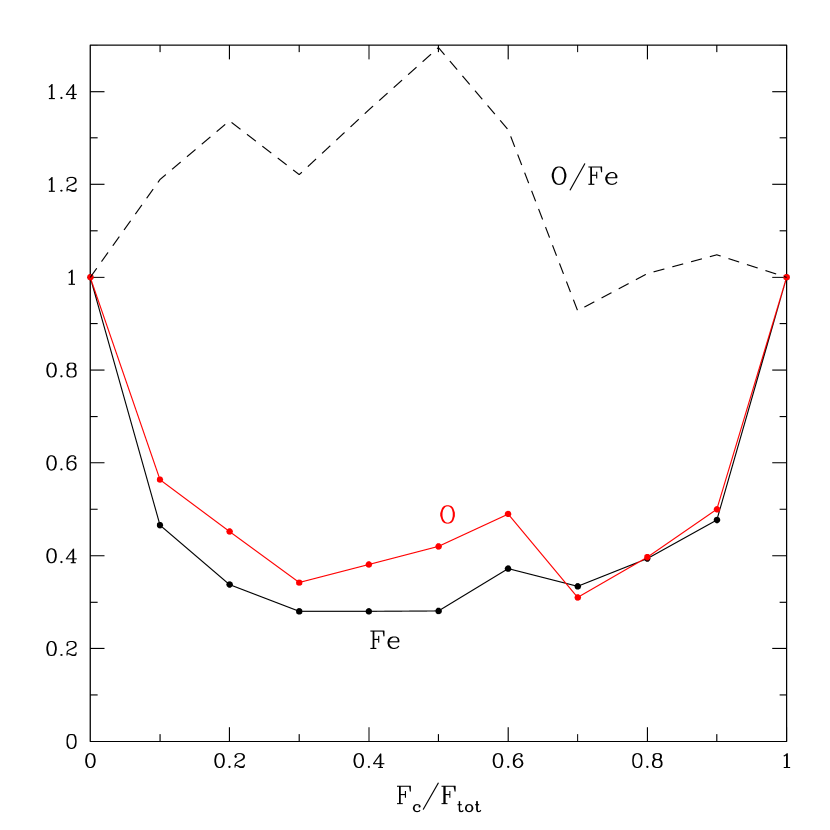
Figure 11: Best-fit values of O, Fe and O/Fe derived from fitting a single temperature model to simulated two-temperature spectra with a lower temperature of 0.7 keV and an upper temperature of 1.3 keV and a range in flux ratios between the two temperature components. All simulated spectra have solar O and Fe abundances.

Even though the Fe abundance contrast between the low and high abundance regions is significantly reduced by fitting the spectra with a two-temperature model, there is still a clear separation between the high and low abundance regions in the O/Fe and Fe plane (see Figure 10). On average, the low abundance regions have higher O/Fe ratios than those derived for the high abundance regions. To investigate the dependence of the O/Fe ratio on the presence of multiphase gas, we simulated a set of two-temperature spectra and fit the spectra to a single temperature model. All of the simulated two-temperature models have a solar O/Fe ratio, a lower temperature of 0.7 keV, an upper temperature of 1.3 keV and a range in flux ratios between the two temperature components. The spectra were then fit to a single vapec model with O and Fe allowed to vary independently. The results are shown in Fig. 11. This figure shows that the O/Fe ratio can be overestimated by 30-50%, due to the presence of multi-phase gas which can explain the segregation seen in the O/Fe and Fe plane shown in Figure 10, if the gas in the low abundance region has a greater predominance of multiphase gas and the actual O/Fe ratios are similar between the different regions. These results imply that the apparently low abundance regions in the abundance map have a more inhomogeneous gas temperature distribution compared to the apparently high abundance regions, but that the actual Fe abundances and O/Fe ratios are fairly similar.

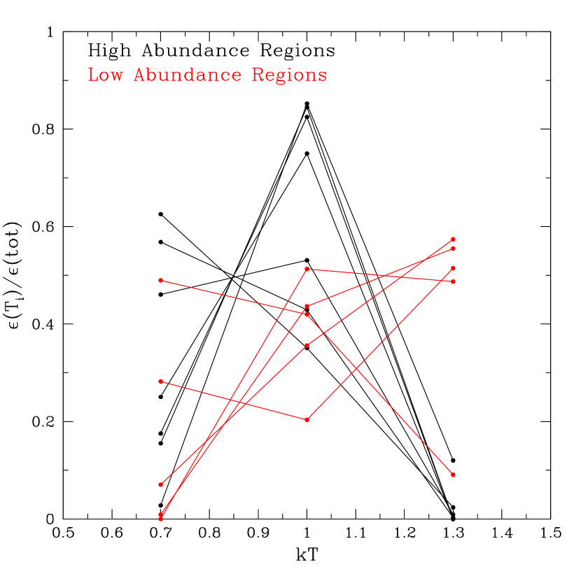
Figure 12: Fractional distribution of the emission measure derived from a three temperature fit (kT=0.7, 1.0 and 1.3 keV) to the spectra from the high and low abundance regions.

To further support the claim that the low abundance regions reside in highly multiphase gas, we fit the spectra to a three temperature model with the temperatures fixed at 0.7, 1.0 and 1.3 keV and the O and Fe abundances linked between the different temperature components. Figure 12 shows the relative distribution of the emission measures for the three temperature components. This figure clearly shows that the low abundance regions have a broader temperature distribution of emission measures compared to that among the high abundance regions.

In summary, there are four reasons to suspect that the apec derived abundance map shown in Figure 4 is more a map of temperature inhomogeneities rather than a true abundance map. These are: 1) the higher values of $F_{c}/F_{tot}$ in the high abundance regions compared to the low abundance regions, 2) the narrower temperature distribution in the emission measures within the high abundance regions compared to that in the low abundance regions, 3) the greater increase in the derived Fe abundance in the low abundance regions compared to the high abundance regions when a second temperature component is added and 4) the smaller values of the O/Fe ratio in the high abundance regions compared to that in the low abundance regions derived from a single temperature analysis.

5 Abundance Profiles

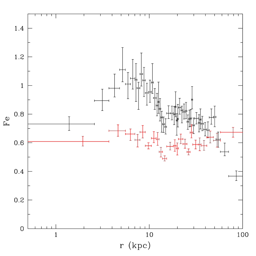
Figure 13: Projected Fe abundance profile relative to the solar value in Grevesse & Sauval (1998). All spectra were fit to absorbed single temperature models vapec with $N_{H}$ frozen at the galactic value. The black data points are the best fit Fe abundances with all of the elemental abundances linked together. The red data points are the best fit Fe abundances with O allowed to vary independently of Fe. Spectra with 10,000 net counts each were used to generate the black data points and spectra with 20,000 net counts each were used to generate the red data points.

The model-dependent nature of derived abundances for emission from multiphase gas with non-solar abundance ratios makes it difficult to determine azimuthally averaged abundance profiles. Such information is essential for determining the masses and mass ratios of different elements and the relative enrichment from Type Ia and Type II supernovae. To study the sensitivity of derived abundance profiles on the assumed spectral model, we produced 3 sets of spectra (with 10000, 20000 and 40000 net counts in each spectrum) extracted from concentric annuli centered on NGC 5044. Figure 13 shows the projected Fe abundance profile derived by fitting an absorbed vapec model with all the elemental abundances linked to Fe (this is equivalent to fitting the spectra to an apec model). Also shown in Figure 13 is the projected Fe abundance profile if the O and Fe abundances are allowed to vary independently. The presence of non-solar abundance ratios produces a sharp peak in the Fe abundance if all of the elements are linked together. Allowing the O abundance to vary produces a fairly flat Fe abundance profile within the central 100 kpc.

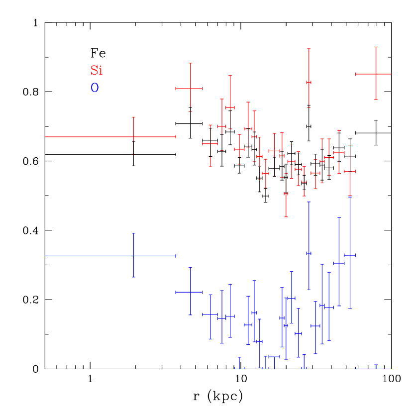
Figure 14: Projected O, Si and Fe abundance profiles relative to the solar values in Grevesse & Sauval (1998). All spectra have 20,000 net counts each and were fit to absorbed single temperature models (vapec) with $N_{H}$ frozen at the galactic value.

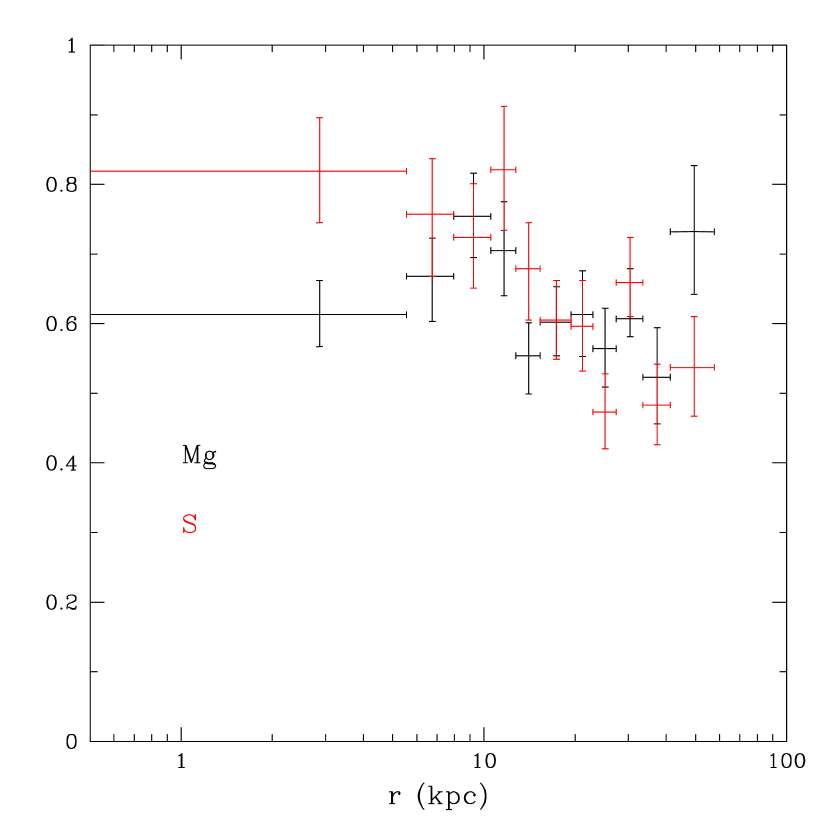
Figure 15: Projected Mg and S abundance profiles relative to the solar values in Grevesse & Sauval (1998). All spectra have 40,000 net counts each and were fit to absorbed single temperature models (vapec) with $N_{H}$ frozen at the galactic value.

To investigate the distribution of other elements, we also fit the sets of spectra with 20000 and 40000 net counts to an absorbed vapec model with O, Mg, Ne, Si, S and Fe treated as free parameters. Figure 14 shows the projected Fe, Si and O abundance profiles and Figure 15 shows the projected Mg and S abundance profiles. We do not show the Ne abundances due to their large uncertainties. Figures 14 and 15 show, that except for O, the other elements have essentially solar ratios. This explains why the spectral analysis of the low and high abundance regions analyzed in $\S 6$ did not improve significantly when elements other than O were allowed to vary independently of Fe.

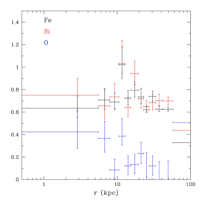
Figure 16: Deprojected Fe, Si and O abundance profiles relative to the solar values in Grevesse & Sauval (1998). All spectra have 40000 net counts each and were fit to absorbed single temperature models (vapec) with $N_{H}$ frozen at the galactic value.

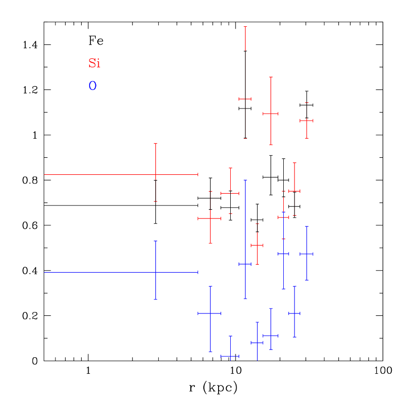
Figure 17: Deprojected Fe, Si and O abundance profiles relative to the solar values in Grevesse & Sauval (1998). All spectra have 40000 net counts each and were fit to absorbed two-temperature models with $N_{H}$ frozen at the galactic value.

The deprojected Fe, O and Si abundance profiles derived from fitting single and two-temperature models are shown in Figures 16 and 17. The spectra were deprojected using the XSPEC task projct. These figures show that there is little difference between the projected and deprojected Fe and Si abundance profiles, since they are both essentially flat within the central 100 kpc. The O/Fe ratio is also significantly less than the solar ratio for both the single and two-temperature deprojections.

6 Comparison with XMM-Newton EPIC and RGS Results

Buote et al. (2003) derived azimuthally averaged abundance profiles for NGC 5044 from a joint analysis of an earlier 20 ksec Chandra observation and an XMM-Newton observation. They found significant improvements in the spectral analysis when the data were fit with two-temperature or differential emission measure models compared to single temperature models and discussed the sensitivity of the derived abundances on the presence of multiphase gas. Most of their abundance profiles have a peak abundance between 10-30 kpc with lower values both interior and exterior to this region. The peak abundances in their profiles correspond to the ring of high abundance clouds seen in the abundance map (see Figure 2). The peak Fe abundances in Buote et al. are approximately 0.8 and 1.2 solar in the projected and deprojected analysis, which are in good agreement with the results presented here.

Tamura et al. (2003) presented an analysis of the XMM-Newton Reflection Grating Spectrometer (RGS) observation of NGC 5044 and found that the emission within the central $2^{\prime}$ (22 kpc) was well fit by a two-temperature model with temperatures of 0.7 and 1.1 keV (consistent with the range in temperatures along the line-of-sight), an Fe abundance of 0.55 and an oxygen abundance of 0.25 (relative to the abundance table in Anders & Grevesse 1989). Converting these values using the abundance table in Grevesse & Sauval (1998) gives Fe=0.81 and O/Fe=0.39. These values for the Fe abundance and O/Fe ratio fall between the values for the high and low abundance regions in Figure 10.

7 H$\alpha$ emission

A narrow-band H$\alpha$ image of NGC 5044 was obtained on April 10, 2010 with the 4.1 m Southern Observatory for Astrophysical Research (SOAR) telescope using the SOAR Optical Imager (SOI). Two CTIO narrow-band filters were used: 6649/76 for the H$\alpha$+[NII] lines and 6520/76 for the continuum. Each image was reduced using the standard procedures in the IRAF MSCRED package and the spectroscopic standard is LTT 3864. More details on the SOI data reduction can be found in Sun et al. (2007).

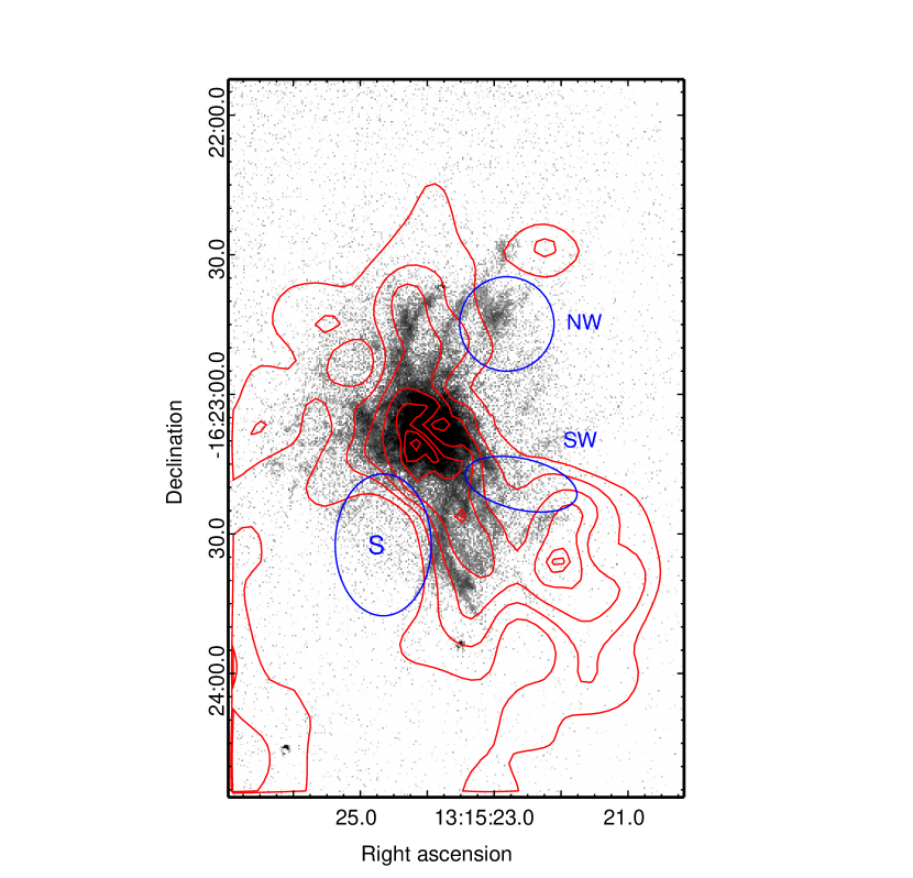
Figure 18: H$\alpha$ image along with temperature contours (red curves) derived from the temperature map shown in Figure 1, The gas temperatures increase from the smallest to the largest contours. Also shown are the southern, northwestern and southwestern cavities (blue curves).

Figure 18 shows the H$\alpha$ emission along with gas temperature contours (red) and the locations of the southern, northwestern and southwestern caviities (blue). The total H$\alpha$ flux and luminosity is $\sim 4.4\times 10^{-13}$ erg cm^-2 s^-1 and $\rm{L_{H\alpha}}\sim 7.9\times 10^{40}$ erg s^-1. The H$\alpha$ emission is primarily extended in a north-south direction, as previously reported by Macchetto et al. (1996). Figure 18 shows that there are many emission-line filaments extending at least 10 kpc from the nucleus. Most of the filaments extend toward the NW cavity and along the SW filament, which is located between the SW and S cavities. There is a clump of H$\alpha$ emission within the NW cavity and some H$\alpha$ emission in the SW cavity, but very little emission within the southern cavity. Both the NW and SW cavities are radio quiet based on our recent GMRT observations. The brightest and longest of the southern H$\alpha$ filaments borders the western edge of the southern cavity. The temperature contours in Figure 18 show that there is a strong correlation between the location of the coolest X-ray emitting gas and the H$\alpha$ emission. Temi et al. (2007) reported evidence for distributed PAH emission with the same morphology as the southern extension of the H${\alpha}$ emission based on a Spitzer observation of NGC 5044.

As discussed in Paper I, the kinematics of the H${\alpha}$ emitting gas are inconsistent with an external origin for the gas (Caon et al. 2000) and are similar to the kinematics of the H${\alpha}$ filaments in NGC 1275 (Hatch et al. 2006). We also showed in paper I that the most likely origin for the H${\alpha}$ emitting gas was due cooling of the hot X-ray emitting gas since the stellar mass loss rate in NGC 5044 is more than an order magnitude less than the mass cooling rate. All of these results are consistent with a scenario in which the gas responsible for the H${\alpha}$ originates from cooling of the hot X-ray emitting gas within the central few kpcs of NGC 5044, followed by dredge up behind AGN-inflated, buoyantly rising bubbles. The SW H$\alpha$ filament is apparently being dredged up along the outer edge of the 235 MHz radio emitting plasma which threads the southern cavity (see Paper I).

8 Discussion

The multiphase gas in the center of NGC 5044 is likely produced by AGN induced stirring or turbulence. If all AGN activity were to cease, then the subsequent cascading of the turbulence to smaller scales and the eventual dissipation of the turbulent kinetic energy into heat, along with thermal conduction, will eventually produce a more homogeneous distribution of gas temperature. Turbulent kinetic energy is dissipated on approximately the eddy turnover time of the largest eddy which is given by $t_{eddy}=l/u$, where $l$ is the length scale of the largest eddy and $u$ is corresponding turbulent velocity. The dissipation rate of turbulent kinetic energy per unit volume is given by (e.g., David & Nulsen 2008):

$$\Gamma_{diss}=c_{2}\rho_{g}u^{2}/t_{eddy}=c_{2}\rho_{g}l^{2}/t_{eddy}^{3}$$ (1)

where $c_{2}$ is a constant of order unity and $\rho_{g}$ is the gas density. We can estimate $t_{eddy}$ by assuming that the dissipation rate of turbulent kinetic energy locally balances radiative losses, i.e., $\Gamma_{diss}=\Delta L_{bol}$, where $\Delta L_{bol}$ is the bolometric luminosity of the gas per unit volume. Assuming the turbulence can be characterized by a local mixing length prescription, then the size of the largest eddies can be written as $l=\alpha r$, where $\alpha$ is a parameter between 0 and 1 and $r$ is the radial distance from the cluster center. Substituting these expressions into eq. (1) and solving for $t_{eddy}$ gives:

$$t_{eddy}=\left({{c_{2}\alpha^{2}r^{2}\rho_{g}}\over{\Delta L_{bol}}}\right)^{1/3}$$ (2)

Adopting $c_{2}=0.42$ (based on the discussion in Dennis & Chandran 2005), we computed $t_{eddy}$ as a function of radius for NGC 5044 for $\alpha=0.2$ and $0.5$ (see Figure 19). This figure shows that without further AGN outbursts, the kinetic energy associated with the present level of turbulence will be thermalized within approximately $10^{8}$ yr within the central 10 kpc. The required turbulent velocity to locally balance radiative losses within the central 10 kpc is $u\sim 20-40$ km s^-1 for $\alpha=0.2-0.5$, which gives a turbulent gas pressure less than 1% of the thermal gas pressure within this region.

A cool cloud embedded in hotter gas will be heated by thermal conduction at a rate (see the discussion in Voit et al. 2008):

$$H=4\pi r_{c}^{2}f_{s}\kappa(T)\Delta T/r_{c}$$ (3)

where $r_{c}$ is the radius of the cool cloud, $\Delta T$ is the temperature difference between the cool cloud and the ambient medium, $f_{s}$ is a reduction factor relative to Spitzer conduction and $\kappa(T)=6\times 10^{-7}T^{5/2}$ erg s^-1 K^-1 cm^-1. The time scale for conduction to heat the cool cloud to the ambient gas temperature at constant pressure is:

$$t_{cond}={{5k\Delta TM_{c}}\over{2\mu m_{p}H}}$$ (4)

where $M_{c}$ is the mass of the cool cloud. This equation can be written as:

$$t_{cond}={{5kr_{c}^{2}\rho_{c}}\over{6\mu m_{p}f_{s}\kappa(T)}}$$ (5)

where $\rho_{c}$ is the gas density within the cool cloud. The conduction time scale as a function of radius is shown in Fig. 19 assuming a 20% difference between the gas temperature in the cool cloud and ambient medium, or equivalently, a 20% contrast in density, assuming the clouds are in pressure equilibrium, $r_{c}=1$ kpc and $f_{s}=0.1$ or $0.3$. This figure shows that $t_{cond}$ is comparable to $t_{eddy}$ within the central 10 kpc. The conduction time scale declines beyond the central 10 kpc due to the increasing gas temperature (see the temperature profile presented in Paper I) and the $T^{5/2}$ factor in the heat conduction rate.

Figure 19 shows that both turbulence and heat conduction will produce a more homogeneous distribution of gas temperature within the central 10 kpc in NGC 5044 within approximately $10^{8}$ yr in the absence of continued AGN driven turbulence. The fact that there is multiphase gas within this region implies that the delay between recent AGN outbursts has been less than $10^{8}$ yr.

While conduction may be efficient at re-heating small cool clouds beyond the central 10 kpc in NGC 5044 (see Figure 19), conduction has a negligible affect on preventing the bulk of the central gas in NGC 5044 from cooling. Figure 20 shows the value of $f_{s}$ required for heat conduction to locally balance radiative losses. Within the central 20 kpc, where the gas is fairly isothermal, heat conduction rates in excess of the Spitzer value are required to suppress cooling. Beyond 50 kpc, near the peak in the temperature profile, heat conduction actually helps to cool the gas (negative values of $f_{s}$), since the divergence of the heat flux is negative in this region. Thus, there is only a small range in radii, between 25-50 kpc, where heat conduction could be important in preventing the gas from cooling.

9 Summary

In Paper I, we showed that the central region of NGC 5044 has been strongly perturbed by at least three recent AGN outbursts. By combining GMRT and Chandra data, we found direct evidence for the uplifting of low entropy gas from the center of NGC 5044 by AGN-inflated, radio emitting X-ray cavities. The nearly continuous production of AGN-inflated bubbles over the past few $10^{8}$ years has probably produced some gas turbulence within the central regions of NGC 5044. This AGN driven turbulence can have a significant impact on the distribution of heavy elements and the production and longevity of multiphase gas in the center of NGC 5044.

In this paper, we have shown that fitting a single temperature thermal plasma model with the ratios of the elemental abundances fixed at the solar values (e.g., apec) can produce significant artifacts in abundance maps. To investigate the origins of the artifacts in the apec derived abundance map for NGC 5044, we extracted spectra from several regions with apparently high and low abundances and fit these spectra to a variety of spectral models with different combinations of free parameters. The single greatest improvement in the spectral analysis was obtained by fitting the spectra with a vapec model with the O and Fe abundances allowed to vary independently. For the apparently high abundance regions, the best-fit Fe abundances derived with the vapec model are significantly less than the abundances obtained with the apec model. These high abundance regions also have best-fit values of the O/Fe ratio significantly less that the solar value. For the apparently low abundance regions, the best-fit Fe abundances derived with the vapec model are essentially consistent with the abundances derived with the apec model. The low abundance regions have near solar O/Fe ratios. Freeing up the abundance of other heavy elements does not further improve the spectral fits in any of the extracted spectra, indicating that the abundance ratios of the other elements are essentially consistent with the solar ratios. This analysis showed that a substantial portion of the artifacts in the apec derived abundance map are due to the enforcement of a solar O/Fe ratio in the spectral analysis. This result was confirmed by generating a set of simulated vapec spectra with a range of O/Fe values and fitting the data to an apec model. We found that the best-fit abundance obtained with an apec model increases with a decreasing O/Fe ratio.

After allowing for non-solar O/Fe values in the spectral analysis, the next greatest single improvement in the quality of the spectral fits was obtained by including a second temperature component. The addition of a second temperature component produces a slight increase in the Fe abundance in the apparently high abundance regions and a much greater increase in the Fe abundance in the apparently low abundance regions. The O/Fe ratios are consistent between the single and two temperature spectral analysis, given the uncertainties. The flux from the second temperature component in the apparently high abundance regions is consistent with that expected from projection affects given the deprojected temperature profile of NGC 5044. For the spectra extracted from the regions with apparently low abundances, the emission from the two different temperature components is more evenly distributed. In addition to fitting the spectra to a two temperature model, we also fit the spectra to a three temperature model with the temperatures fixed at 0.7, 1.0 and 1.3 keV. This analysis showed that the emission from the apparently low abundance regions is more evenly distributed among the different temperature components compared to the emission from the apparently high abundance regions, confirming that inhomogeneities in the temperature distribution are partly responsible for producing the artifacts in the apec derived abundance map. We also found that excess absorption and emission from unresolved LMXBs cannot produce the artifacts observed in the apec derived abundance map.

We have shown that deprojected abundance profiles are very sensitive to the assumed spectral model. A single temperature apec model produces a deprojected abundance profile for NGC 5044 that increases by a factor of approximately 2 from 100 to 10 kpc, and then decreases inward. By fitting the same set of spectra with a vapec model with the O and Fe abundances allowed to vary independently, we obtain deprojected O and Fe abundance profiles that are fairly uniform within the central 100 kpc. Central dips in abundance profiles are a fairly common occurrence in cooling flow clusters (e.g., Sanders et al. 2004, Churazov et al. 2004). Our results show that such dips in the central abundance profile could be due to non-solar ratios of the heavy elements or the presence of multiphase gas. Excluding oxygen, all of the other elements that produce strong emission lines in 1 keV gas (i.e., Mg, Si and S) have essentially flat abundance profiles with near solar ratios within the central 100 kpc.

The O/Fe ratio is a useful diagnostic for determining the relative enrichment from Type Ia and Type II supernovae. However, estimates of the O/Fe ratio are very sensitive to the presence of multiphase gas. By generating a set of simulated spectra, we have shown that the O/Fe ratio can be overestimated by factors of 2 to 3 when the emission from multiphase gas is fit with a single temperature model. While the uncertainties on the O/Fe ratios obtained from our spectral analysis are fairly large when more than one temperature component is included in the spectral analysis, on average, we find significantly sub-solar values of O/Fe within the central 100 kpc of NGC 5044. This implies a greater relative enrichment from Type Ia enrichment compared to solar abundance gas which is consistent with previous studies of the central regions in groups and clusters (e.g., Finoguenov et al. 2000;2001).

The multiphase gas in NGC 5044 is probably produced by AGN induced turbulence. We have shown that without further AGN outbursts, the gas in the center of NGC 5044 should acquire a more homogeneous distribution of temperature within $10^{8}$ yr due to the dissipation of turbulent kinetic energy and the effects of thermal conduction. The fact that there is a significant component of multiphase gas in the center of NGC 5044 shows that the delay between successive AGN outbursts must be less than $10^{8}$ yr. We have recently obtained deeper GMRT data for NGC 5044 to better probe the past AGN history in this system and we will present the results in a subsequent paper.

We would like to acknowledge Seth Bruch for obtaining the narrow band H$\alpha$+[NII] images at the SOAR. This work was supported by grants GO8-9122X and GO0-11003X. EOS acknowledges the support of the European Community under the Marie Curie Research Traning Network.

Figure 7: Best-fit abundance (Z) derived from fitting an apec model to simulated spectra generated from a vapec model with a solar Fe abundance and a range of O/Fe values.

Figure 8: Best-fit O/Fe ratios derived from fitting an absorbed apec model with the absorption frozen at the galactic value to simulated spectra generated from a vapec model with a solar O/Fe ratio and a range of excess absorption ($\Delta N_{H}$).

Figure 9: Cumulative fraction of the 0.5-3.0 keV X-ray flux, relative to the total flux, as a function of gas temperature along three different projected distances, b, from the center of NGC 5044.

Figure 10: Scatter plot of the O/Fe ratios and Fe abundances for the high abundance clouds (black) and low abundance regions (red) derived from fitting the spectra to a two-temperature vapec model (see Table 5). All error bars are shown at $1\sigma$.

Figure 19: Eddy turnover time assuming that the dissipation of turbulent kinetic energy locally balances radiative losses for $\alpha=0.2$ (lower solid curve) and $\alpha=0.5$ (upper solid curve). Conduction timescale ($t_{cond}$) to re-heat an embedded cool cloud to the ambient gas temperature assuming $f_{s}=0.3$ (lower dashed curve) and $f_{s}=0.1$ (upper dashed curve).

Figure 20: Ratio of the heat flux required to locally balance radiative losses to the Spitzer value for the heat flux.

Table 1: Spectral Analysis Results using an absorbed apec Model

Region	kT	Z	$\chi^{2}$	DOF	$\chi_{\nu}^{2}$
	(keV)	(solar)
H1	1.01 (1.00-1.02)	1.46 (1.23-1.65)	109.7	90	1.22
H2	0.93 (0.92-0.94)	1.31 (1.15-1.46)	201.2	103	1.95
H3	0.82 (0.81-0.83)	1.12 (1.05-1.25)	282.0	118	2.39
H4	0.89 (0.88-0.90)	1.47 (1.19-1.88)	83.4	71	1.17
H5	0.79 (0.78-0.80)	1.29 (1.13-1.50)	157.5	100	1.57
H6	0.78 (0.77-0.79)	1.63 (1.39-2.57)	105.0	74	1.42
H7	0.93 (0.92-0.94)	1.29 (1.02-1.57)	71.1	64	1.11
L1	0.81 (0.80-0.82)	0.73 (0.69-0.81)	154.3	109	1.42
L2	1.06 (1.05-1.07)	0.55 (0.51-0.65)	74.0	74	1.00
L3	0.97 (0.95-0.99)	0.39 (0.34-0.44)	109.5	78	1.40
L4	1.07 (1.05-1.09)	0.53 (0.48-0.59)	91.6	84	1.09
L5	1.06 (1.05-1.07)	0.54 (0.50-0.59)	131.2	106	1.24

Notes: Spectral analysis results for the high and low abundance regions highlighted in Figure 7. All spectra were fit in the 0.5-3.0 keV energy band to a phabs*apec XSPEC spectral model with the absorption frozen at the galactic value ($N_{H}=4.94\times 10^{20}$ cm^-2) and the Grevesse & Sauval (1998) abundance table. This table gives the best-fit temperature (kT), abundance (Z), total $\chi^{2}$, degree of freedom (DOF) and $\chi_{\nu}^{2}$, along with the $1\sigma$ errors.

Table 2: Spectral Analysis Results using an absorbed vapec Model

Region	kT	Fe	O	$\chi^{2}$	DOF	F-Test Prob.
	(keV)	(solar)	(solar)
H1	1.00 (0.99-1.01)	0.92 (0.81-1.04)	0.29 (0.11-0.50)	96.4	89	$7.2\times 10^{-4}$
H2	0.91 (0.90-0.92)	0.70 (0.66-0.74)	0.00 ($<0.05$)	129.8	102	$2.5\times 10^{-11}$
H3	0.80 (0.79-0.82)	0.69 (0.65-0.74)	0.08 (0.03-0.16)	188.9	117	$8.3\times 10^{-12}$
H4	0.88 (0.86-0.89)	0.73 (0.64-0.87)	0.03 ($<0.23$)	76.4	70	$1.2\times 10^{-4}$
H5	0.78 (0.77-0.79)	0.72 (0.67-0.81)	0.10 (0.03-0.22)	112.6	99	$8.9\times 10^{-9}$
H6	0.77 (0.76-0.78)	0.95 (0.81-1.13)	0.34 (0.17-0.57)	91.0	73	$1.3\times 10^{-3}$
H7	0.93 (0.91-0.94)	1.08 (0.92-1.32)	0.89 (0.52-1.43)	70.8	63	0.61
L1	0.80 (0.79-0.81)	0.61 (0.57-0.66)	0.26 (0.18-0.36)	134.5	108	$1.2\times 10^{-3}$
L2	1.06 (1.05-1.07)	0.53 (0.47-0.62)	0.29 (0.17-0.56)	73.7	73	0.59
L3	0.97 (0.95-0.99)	0.40 (0.34-0.46)	0.30 (0.11-0.53)	107.2	77	0.20
L4	1.07 (1.05-1.09)	0.50 (0.44-0.56)	0.30 (0.09-0.52)	89.5	83	0.17
L5	1.06 (1.05-1.09)	0.51 (0.46-0.56)	0.27 (0.11-0.42)	128.3	105	0.13

Notes: All spectra were fit in the 0.5-3.0 keV energy band to a phabs*vapec XSPEC spectral model with the absorption frozen at the galactic value and the O and Fe abundances treated as free parameters. See the notes to Table 1 for further details.

Table 3: Spectral Analysis Results Using an Absorbed apec Model in the 0.8-3.0 keV Band

Region	kT	Z	$\chi^{2}$	DOF
	(keV)	(solar)
H1	1.01 (1.00-1.02)	1.04 (0.91-1.32)	84.8	73
H2	0.91 (0.90-0.93)	0.70 (0.62-0.80)	94.3	83
H3	0.80 (0.79-0.81)	0.63 (0.58-0.69)	154.9	98
H4	0.88 (0.87-0.89)	0.73 (0.58-0.93)	48.5	59
H5	0.78 (0.77-0.79)	0.73 (0.65-0.85)	91.1	80
H6	0.76 (0.75-0.77)	0.97 (0.82-1.41)	70.6	59
H7	0.93 (0.92-0.94)	1.17 (0.89-1.62)	58.6	52
L1	0.81 (0.80-0.82)	0.59 (0.53-0.64)	111.7	89
L2	1.06 (1.05-1.07)	0.47 (0.40-0.54)	68.2	61
L3	0.99 (0.97-1.01)	0.39 (0.29-0.43)	70.1	62
L4	1.05 (1.04-1.06)	0.36 (0.31-0.42)	69.7	69
L5	1.07 (1.06-1.08)	0.52 (0.47-0.59)	102.3	86

Notes: All spectra were fit in the 0.8-3.0 keV energy band to a phabs*apec XSPEC spectral model with the absorption frozen at the galactic value. See the notes to Table 1 for further details.

Table 4: Spectral Analysis Results Using using an Absorbed vapec Model with Free Absorption

Region	kT	Fe	O	$\rm{N_{H}}$	$\chi^{2}$	DOF	F-Test Prob.
	(keV)	(solar)	(solar)	$(10^{20}cm^{2})$
H1	1.00 (0.99-1.01)	0.92 (0.81-1.04)	0.27 (0.06-0.54)	4.73 (2.98-6.54) (1.92-7.74)	96.4	88	1.00
H2	0.91 (0.90-0.92)	0.67 (0.63-0.73)	0.00 ($<0.05$)	6.09 (5.39-7.18) (4.10-7.94)	129.0	101	0.43
H3	0.79 (0.78-0.80)	0.71 (0.66-0.76)	0.19 (0.11-0.28)	7.62 (6.73-8.53) (6.17-9.12)	179.4	116	0.010
H4	0.84 (0.83-0.85)	0.73 (0.62-0.88)	0.12 ($<0.42$)	9.36 (7.19-11.7) (5.74-13.4)	63.3	69	$3.3\times 10^{-4}$
H5	0.77 (0.76-0.78)	0.76 (0.68-0.86)	0.22 (0.09-0.37)	7.24 (5.87-8.62) (5.00-9.63)	109.8	98	0.11
H6	0.76 (0.75-0.77)	0.98 (0.84-1.40)	0.45 (0.24-1.07)	7.13 (5.90-9.95) (3.75-11.7)	90.0	72	0.37
H7	0.93 (0.91-0.95)	1.07 (0.88-1.33)	0.82 (0.41-1.47)	4.22 (1.71-6.92) (1.94-8.70)	70.7	62	0.88
L1	0.80 (0.79-0.81)	0.64 (0.59-0.69)	0.37 (0.25-0.50)	6.90 (5.80-7.97) (5.12-8.02)	131.2	107	0.10
L2	1.05 (1.04-1.07)	0.55 (0.48-0.65)	0.46 (0.20-0.88)	7.14 (5.04-9.60) (3.55-11.4)	72.7	72	0.33
L3	0.95 (0.93-0.97)	0.41 (0.34-0.48)	0.54 (0.24-0.86)	8.25 (5.88-10.6) (3.45-4.86)	105.3	76	0.24
L4	1.05 (1.03-1.07)	0.52 (0.46-0.64)	0.72 (0.41-1.25)	10.7 (8.53-13.2) (6.90-15.4)	83.3	82	0.015
L5	1.06 (1.04-1.08)	0.51 (0.46-0.56)	0.35 (0.16-0.55)	6.13 (4.60-7.68) (3.64-8.76)	127.8	104	0.51

Notes: All spectra were fit in the 0.5-3.0 keV energy band to a phabs*vapec XSPEC spectral model with free absorption. See the notes to Table 1 for further details. Both $1\sigma$ and 90% uncertainties are given for $N_{\rm H}$.

Table 5: Spectral Analysis using a two-temperature vapec model

Region	$\rm{kT_{c}}$	$\rm{kT_{h}}$	Fe	O	$\rm{F_{c}/F_{tot}}$	$\chi^{2}$	DOF	F-Test Prob.
	(keV)	(keV)	(solar)	(solar)
H1	1.00 (0.99-1.01)	-	0.92 (0.81-1.04)	0.27 (0.06-0.54)	-	-	-	-
H2	0.83 (0.82-0.85)	1.22 (1.11-1.33)	0.87 (0.78-0.96)	0.00 ($<0.07)$	0.75	115.0	100	$2.40\times 10^{-3}$
H3	0.78 (0.77-0.79)	1.36 (1.24-1.47)	1.00 (0.90-1.06)	0.29 (0.21-0.34)	0.89	154.9	115	$1.12\times 10^{-5}$
H4	0.80 (0.52-0.85)	1.00 (0.90-1.08)	0.95 (0.78-1.17)	0.06 ($<0.27)$)	0.88	57.7	68	$7.37\times 10^{-5}$
H5	0.77 (0.76-0.77)	2.30 (1.76-3.23)	1.08 (0.98-1.25)	0.36 (0.25-0.66)	0.93	100.2	97	$3.57\times 10^{-3}$
H6	0.74 (0.67-0.76)	1.30 (0.96-1.57)	1.51 (1.04-2.40)	0.78 (0.49-1.29)	0.90	85.1	71	0.092
H7	0.93 (0.91-0.95)	-	1.07 (0.88-1.33)	0.82 (0.41-1.47)	-	-	-	-
L1	0.76 (0.74-0.77)	1.21 (1.10-1.35)	0.98 (0.86-1.13)	0.60 (0.45-0.77)	0.78	91.5	106	$1.35\times 10^{-9}$
L2	0.97 (0.91-1.02)	1.36 (1.20-1.71)	0.85 (0.70-1.24)	0.71 (0.42-1.18)	0.60	67.5	71	0.044
L3	0.71 (0.63-0.79)	1.23 (1.15-1.37)	0.78 (0.71-1.00)	0.62 (0.23-0.98)	0.40	82.0	75	$1.61\times 10^{-4}$
L4	1.07 (1.05-1.09)	-	0.50 (0.44-0.56)	0.30 (0.09-0.52)	-	-	-
L5	0.62 (0.27-0.71)	1.16 (1.12-1.19)	0.77 (0.65-0.86)	0.46 (0.16-0.64)	0.13	110.2	103	$3.97\times 10^{-4}$

Notes: All spectra were fit in the 0.5-3.0 keV energy band to a phabs*(vapec+vapec) XSPEC spectral model with the absorption frozen at the galactic value. The lower best-fit temperature is given by $\rm{kT_{c}}$ and the upper best-fit temperature is given by $\rm{kT_{h}}$. The ratio between the fluxes in the cooler spectral component to the total flux in the 0.5-3.0 keV energy band is given by $\rm{F_{c}/F_{tot}}$. See the notes to Table 1 for further details.

References

- (1) Buote, D. 1999, MNRAS, 309, 685.
- (2) Buote, D., Lewis, A., Brighenti, F. & Mathews, W. 2003, ApJ, 595, 151.
- (3) Caon, N., Macchetto, D. & Pastoriza, M. 2000, ApJSuppl, 127, 39.
- (4) Chandran, B. 2005, ApJ, 632, 809.
- (5) Churazov, E., Forman, W., Jones, C., Sunyaev, R. & Böhringer, H. 2004, MNRAS, 347, 29.
- (6) Croton, D., Springel, V., White, S., De Lucia, G., Frenk, C., Gao, L., Jenkins, A., Kauffmann, G., Navarro, J., Yoshida, N. 2006, MNRAS, 365, 11.
- (7) David, L. & Nulsen, P.E.J. 2008, ApJ, 689, 837.
- (8) David, L., Jones, C., Forman, W., Nulsen, P., Vrtilek, J., O’Sullivan, E., Giacintucci, S. & Raychaudhury, S. 2009, ApJ, 705, 624.
- (9) Finoguenov, A., David, L. & Ponman, T. 2000, ApJ, 188, 203.
- (10) Finoguenov, A., Reiprich, T. & Bohringer, H. 2001, A&A, 368, 749.
- (11) Gebhardt, K. et al. 2000, ApJ, 539, L13.
- (12) Giacintucci, S., O’Sullivan, E., Vrtilek, J., Raychaudhury, S., David, L., Venturi, T., Athreya, R., Murgia, M.& Ishwara-Chandra, C. 2010, ApJ, (submitted).
- (13) Gitti, M., O’Sullivan, E., Giacintucci, S., David, L., Vrtilek, J., Raychaudhury, S.& Nulsen, P. 2010, ApJ, (in press).
- (14) Grevesse, N. & Sauval, A. 1998, Sp. Sci. Rev.,.85, 161.
- (15) Hatch, N., Crawford, C., Johnstone, R., Fabian, A. 2006, MNRAS, 367, 433.
- (16) Macchetto, F., Pastoriza, M., Caon, N., Sparks, W., Giavalisco, M., Bender, R., Capaccioli, M. 1996, A&A Suppl., 120, 463.
- (17) McNamara, B. & Nulsen, P. 2007, ARA&A, 45, 117.
- (18) O’Sullivan, E., Vrtilek, J., Kempner, J., David, L. & Houck, J. 2005, MNRAS, 357, 1134.
- (19) Peterson, J. & Fabian, A. 2006, Phys Rep., 427, 1.
- (20) Rasia, E., Mazzotta, P., Bourdin, H., Borgani, S., Tornatore, L., Ettori, S., Dolag, K. & Moscardini, L. 2008, ApJ, 674, 728.
- (21) Sanders, J., Fabian, A., Allen, S. & Schmidt, R. 2004, MNRAS, 349, 952.
- (22) Sun, M., Donahue, M. & Voit, G. M. 2007, ApJ, 671, 190.
- (23) Tamura, T., Kaastra, J., Makishima, K. & Takahashi, I. 2003, A&A, 399, 497.
- (24) Temi, P., Brighenti, F. & Mathews, W. 2007, ApJ, 666, 222.
- (25) Voit, G.M., Cavagnolo, K., Donahue, M., Rafferty, D., McNamara, B. & Nulsen, P. 2008, ApJ, 681, L5.