Spin-Glass and other random models Statistical Mechanics of model systems

Low Temperature Mass Spectrum in the Ising Spin Glass

Abstract

We study the spectrum of the Hessian of the Sherrington-Kirkpatrick model near $T=0$, whose eigenvalues are the masses of the bare propagators in the expansion around the mean-field solution. In the limit $T\ll 1$ two regions can be identified. The first for $x$ close to $0$, where $x$ is the Parisi replica symmetry breaking scheme parameter. In this region the spectrum of the Hessian is not trivial, and maintains the structure of the full replica symmetry breaking state found at higher temperatures. In the second region $T\ll x\leq 1$ as $T\to 0$, the bands typical of the full replica symmetry breaking state collapse and only two eigenvalues are found: a null one and a positive one. We argue that this region has a droplet-like behavior. In the limit $T\to 0$ the width of the full replica symmetry breaking region shrinks to zero and only the droplet-like scenario survives.

The physics of spin glasses is still an active field of research because the methods and techniques developed to analyze the static and dynamic properties have found applications in a variety of others fields of the complex system world, such as neural networks or combinatorial optimization or glass physics. In the study of spin glasses a central role is played by the Sherrington-Kirkpatrick (SK) model [1], introduced in the middle of 70’s, as a mean field model for spin glasses. Despite the fact that its solution, known as the “Parisi solution” [2, 3], was found $30$ years ago, some aspect are still far from being completely understood. In this Note we discuss the stability, that is the eigenvalue spectrum of the Hessian of the fluctuations, of the Parisi solution in the $T\ll 1$ and its implications for the Replica Symmetry Breaking (RSB) versus droplet scenarios.

Model.–The model is defined by the Hamiltonian [4]

$$H=-\frac{1}{2}\sum_{i,j}J_{ij}\,s_{i}\,s_{j}$$ (1)

where $s_{i}=\pm 1$ are $N$ Ising spins located on a regular $d$-dimensional lattice and the symmetric bonds $J_{ij}$, which couple nearest-neighbor spins only, are random quenched Gaussian variables of zero mean. The variance is properly normalized to ensure a well defined thermodynamic limit $N\to\infty$. By using the standard replica method to average over the disorder, the free energy density $f$ in the thermodynamic limit can be written as function of the symmetric $n\times n$ site dependent replica overlap matrix $Q_{i}^{ab}$ as $-\beta f=\lim_{n\to 0}\frac{1}{n}\max_{Q}{\cal L}[Q]$ with [5]

$${\cal L}[Q] = -\frac{\beta^{2}}{2}\sum_{\bm{q}}(q^{2}+1)\sum_{(ab)}\,(Q_{\bm{q}}^{ab})^{2}$$ (2)

$$\phantom{==}+\sum_{i}\ln{\rm Tr}\exp\Bigl{(}{\beta^{2}\sum_{(ab)}Q_{i}^{ab}s^{a}s^{b}}\Bigr{)}$$

where $Q_{\bm{q}}^{ab}$ is the spatial Fourier Transform of $Q_{i}^{ab}$ and $\beta=1/T$. The notation “$(ab)$” means that only distinct ordered pairs $a<b$ ($a,b=1,\ldots,n$) are counted. By writing $Q_{i}^{ab}=Q^{ab}+\delta Q_{i}^{ab}$ and expanding ${\cal L}[Q]$ in powers of $\delta Q_{i}^{ab}$ one generates the loop expansion. The site-independent $Q^{ab}$ is given by the mean field value $Q^{ab}=\langle s^{a}s^{b}\rangle$, where angular brackets denote a weighted average with $\exp(\beta^{2}\sum_{(ab)}Q^{ab}s^{a}s^{b})$. This follows from the stationarity of ${\cal L}[Q]$, that is the vanishing of the linear term in the expansion, and ensures that no tadpoles are present. The quadratic term of the expansion defines the bare propagators whose “masses” are given by the eigenvalues of the non-kinetic part of the fluctuation matrix:

$$M^{ab;cd}=\delta_{(ab);(cd)}^{Kr}-\beta^{2}\Bigl{[}\langle s^{a}s^{b}s^{c}s^{d}\rangle-\langle s^{a}s^{b}\rangle\langle s^{c}s^{d}\rangle\Bigl{]}$$ (3)

that is the Hessian matrix of the SK model.

Stability of the Parisi solution for the SK model near its critical temperature $T_{c}$, has been established long ago by exhibiting the eigenvalues of the Hessian matrix [6, 7]. In few words, one has a Replicon band whose lowest masses are zero modes, and a Longitudinal-Anomalous band, sitting at $(T_{c}-T)$, of positive masses, both with a band width of order $(T_{c}-T)^{2}$. The analysis was extended via the derivation of Ward-Takahashi identities [8], showing that the zero Replicon modes would remain null in the whole low temperature phase, and hence would not ruin the stability under loop corrections to the mean field solution.

Despite these efforts a complete analysis of the stability in the zero temperature limit is still missing. Near $T_{c}$ one can take advantage of the vanishing of the order parameter for $T=T_{c}$ and expand ${\cal L}[Q]$, a simplification clearly missing close to zero temperature, where the order parameter stays finite.

Low Temperature Phase.–As the temperature is lowered the ergodicity breaks down at the critical temperature $T_{c}=1$. Below $T_{c}$ the phase of the SK model is characterized by a large, yet not extensive, number of degenerate locally stable states in which the system freezes. The symmetry under replica exchange is broken and the overlap $Q^{ab}$ becomes a non-trivial function of replica indexes. Assuming $R$ steps of RSB the matrix $Q^{ab}$ is divided, following the Parisi parameterization [3], into successive boxes of decreasing size $p_{r}$, with $p_{0}=n$ and $p_{R+1}=1$, with elements given by

$$Q^{ab}=Q_{r},\qquad r=0,\ldots,R+1$$ (4)

where $r=a\cap b$ denotes the overlap between replicas $a$ and $b$. This means that $a$ and $b$ belongs to the same box of size $p_{r}$, but to two distinct boxes of size $p_{r+1}<p_{r}$. The solution of the SK model is obtained by taking $R\to\infty$. In absence of an external field the overlap $Q^{ab}$ takes values between zero and a maximum value $q_{c}(T)\leq 1$, and so for $R\to\infty$ the matrix $Q^{ab}$ is described by a continuous non-decreasing function $Q(x)$ parameterized by the variable $x$. In the Parisi scheme $x\in[0,1]$ and gives the probability for a pair of states to have an overlap $Q^{ab}$ not larger than $Q(x)$.

The meaning of $x$ depends on the parameterization used for the matrix $Q^{ab}$. In the dynamical approach [9, 10, 11] $x$ labels the relaxation time scale $t_{x}$, so that $Q(x)=\langle s(t_{x})\,s(0)\rangle$. Here the angular brackets denotes time (and disorder) averaging. The smaller $x$ the longer $t_{x}$. All time scales diverges in the thermodynamic limit but $t_{x^{\prime}}/t_{x}\to\infty$ if $x>x^{\prime}$. To make contact with the static Parisi solution one takes $x\in[0,1]$, with $x=0$ corresponding to the largest possible relaxation time and $x=1^{-}$ to the shortest one. With this assumption one recovers $Q(0)=0$ and $Q(1^{-})=q_{c}(T)$. In both cases $Q(1)=1$, since it gives the self or equal-time overlap. Other choices are possible, e.g., those used in Refs. [12, 13, 14, 15] to handle the $T\to 0$ limit. We stress however that different choices just give a different parameterization of the function $Q(x)$, but do not change the physics, since the relevant quantities are the possible values $q$ that the function $Q(x)$ can take and their probability distribution $P(q)$. This property is called gauge invariance [9, 16, 12]. In what follows we assume the Parisi parameterization.

It turns out [17, 18] that as the temperature is decreased towards $T=0$ the probability of finding overlaps $Q^{ab}$ sensibly smaller than $q_{c}(T)=O(1)$ vanishes with $T$, while there is a finite probability $x_{c}\simeq 0.524\ldots$ that $Q^{ab}\leq q_{c}(T)$. Thus, since $Q(0)=0$, for $T\ll 1$ the order parameter function $Q(x)$ in the Parisi parameterization develops a boundary layer of thickness $\delta\sim T$ close to $x=0$, as shown in Fig. 1.

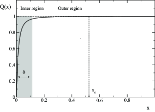
Figure 1: Shape of the order parameter function $Q(x)$ for $T\ll 1$ in the Parisi parameterization. The shaded area shows the extent of the boundary layer of thickness $\delta\sim T$ as $T\to 0$.

From the Figure we see that for very small $T$ the function $Q(x)$ is slowly varying for $\delta\ll x\leq x_{c}$. However, in the boundary layer $0<x\leq\delta$, it undergoes an abrupt and rapid change. In the limit $T\to 0$ the thickness $\delta\sim T\to 0$ and the order parameter function becomes discontinuous at $x=0$.

This behavior of $Q(x)$ for $T\ll 1$ has strong consequences since other relevant quantities, such as, e.g, the four-spin correlation entering into the Hessian matrix, can be computed from partial differential equations of the form,

$$\dot{F}(x,y)=-\frac{\dot{Q}(x)}{2}\Bigl{[}F^{\prime\prime}(x,y)+2\beta\,x\,m(x,y)\,F^{\prime}(x,y)\Bigr{]},$$ (5)

that gives the function $F(x,y)$ for $x<x^{*}$ once $F(x^{*},y)$ is known. Details will be given elsewhere [19]. As usual the “dot” and the “prime” denote derivative with respect to $x$ and $y$, respectively. The function $F(x,y)$ is a generic quantity at the scale $x$ in presence of the frozen field $y$. The function $m(x,y)$ is the local magnetization and it is itself solution of eq. (5) with $F(x,y)=m(x,y)$ and initial condition $m(1,y)=\tanh\beta y$ [12]. In the limit $T\to 0$ we then face a boundary layer problem.

Uniform approximate solutions valid for $T\ll 1$ can be constructed by using the boundary layer theory, that is by studying the problem separately inside (inner region) and outside (outer region) the boundary layer [20]. One then introduces the notion of the inner and outer limit of the solution. The outer limit is obtained by choosing a fixed $x$ outside the boundary layer, that is in $\delta\ll x\leq 1$, and allowing $T\to 0$. Similarly the inner limit is obtained by taking $T\to 0$ with $x\leq\delta$. This limit is conveniently expressed introducing an inner variable $a$, such as $a=x/\delta$, in terms of which the solution is slowly varying inside the boundary layer as $T\to 0$. The inner and outer solutions are then combined together by matching them in the intermediate limit $x\to 0$, $x/\delta\to\infty$ and $T\to 0$.

The inner solution of $Q(x)$ as $T\to 0$ was first computed by Sommers and Dupont in their pioneering work [12] by using the inner variable $a$ defined as $1/(dQ(a)/da)=x/T$ and $T\to 0$, the so called Sommers-Dupont gauge. Recently the inner solution for the order parameter function $Q(x)$ as $T\to 0$ was extensively studied by Oppermann, Sherrington and Schmidt [13, 14, 15] by using as inner variable $a=x/T$, as suggested by the Parisi-Toulouse ansatz [21]. In both cases one finds that the inner solution $Q(a)$ for $T\to 0$ is a smooth function of $a$ varying between $0$ and $q_{c}\simeq 1$.

The outer solution was studied by Pankov [22], who found that in the outer region one has

$$Q(x)\sim 1-c(\beta x)^{-2},\qquad T\ll x\leq x_{c}\ \mbox{\rm and }T\to 0$$ (6)

where $c=0.4108\ldots$. The breakpoint $x_{c}$ is $T$-dependent, however its dependence is rather weak and $x_{c}(T)\sim x_{c}(0)=0.524\ldots$ is a rather good approximation for $T\ll 1$ [18]. From this expression one sees that the variation of the $Q(x)$ in the outer region $[Q(x_{c})-Q(x)]/Q(x)\sim c\left(T/x\right)^{2}$ is indeed rather weak.

More interestingly in his work Pankov has found that for $T\ll x\leq x_{c}$ and $T\to 0$ both the local magnetization $m(x,y)$ and the distribution function $P(x,y)$ of the frozen field $y$ at scale $x$ loose their explicit dependence on the scale variable $x$. This result can be extended to the solution of the generic partial differential equation (5). By using the same notation as Pankov this means that in the outer region the solution of eq. (5) is of the form

$$F(x,y)=\widetilde{F}(z),\ z=\beta xy.$$ (7)

called scaling solution by Pankov. This insensitivity with respect to the scale will allow for a complete diagonalization of the Hessian matrix in the outer region.

The Hessian Matrix.–With $4$ replicas the Hessian (3) is characterized by $3$ overlaps. We can distinguish two cases. The Longitudinal-Anomalous (LA) geometry characterized by $a\cap b=r$, $c\cap d=s$ and, if $r\not=s$, the single cross overlap $t=\max[a\cap c,a\cap d,b\cap c,b\cap d]$:

$$M^{ab;cd}=M_{t}^{r;s},\qquad r,s,t=0,1,\ldots R.$$ (8)

Note that $t=R+1$ if $a=c$ or $a=d$ or $b=c$ or $b=d$. The Replicon geometry where $a\cap b=c\cap d=r$, and one has the two cross-overlaps $u=\max[a\cap c,a\cap d]$ and $v=\max[b\cap c,b\cap d]$ with $u,v\geq r+1$:

$$M^{ab;cd}=M_{u;v}^{r;r},\qquad u,v\geq r+1.$$ (9)

The Hessian is a $\frac{n(n-1)}{2}\times\frac{n(n-1)}{2}$ symmetric matrix that after block-diagonalization becomes a string of $(R+1)\times(R+1)$ blocks along the diagonal for the LA Sector, followed by $1\times 1$ fully diagonalized blocks, for the Replicon Sector [23, 24, 25].

Replicon Sector.–The diagonal elements in the Replicon Sector are given by the double Replica Fourier Transform (RFT) of $M_{u;v}^{r;r}$ with respect the cross-overlaps $u,v$ [23]

$$M_{\hat{k},\hat{l}}^{r;r} = \sum_{u=k}^{R+1}\sum_{v=l}^{R+1}p_{u}p_{v}\Bigl{[}M_{u;v}^{r;r}-M_{u-1;v}^{r;r}$$ (10)

$$\phantom{=====}-M_{u;v-1}^{r;r}+M_{u-1;v-1}^{r;r}\Bigr{]}.$$

In the limit $R\to\infty$ the sums are replaced by integrals and $p_{r}=x(Q_{r})$. To evaluate $M_{\hat{k};\hat{l}}^{r;r}$ we have to compute the matrix elements $M_{u;v}^{r;r}$, that is the four-spin average $\langle s^{a}\,s^{b}\,s^{c}\,s^{d}\rangle$ for the Replicon geometry, by solving equations of the form (5). If $r$ lies in the outer region, that is $p_{r}=x(Q_{r})\gg T$ as $T\to 0$ or, equivalently, for fixed $r\not=0$ and $T\to 0$, then insensitivity with respect to the scale variable implies that $M_{\hat{k};\hat{l}}^{r;r}$ is independent of $k$ and $l$. Thus by exploiting this insensitivity we conclude that

$$M_{\hat{k};\hat{l}}^{r;r}=M_{\widehat{r+1};\widehat{r+1}}^{r;r}=O\left(\frac{1}{R^{2}}\right)\stackrel{{\scriptstyle R\to\infty}}{{=}}0.$$ (11)

The second equality follows from a Ward-Takahashi identity [8]. In the inner region the Replicon spectrum maintains its complexity. However its relevance becomes less and less important as $T$ approaches zero, and vanishes in the limit $T\to 0$ when the thickness of the boundary shrinks to zero. The Replicon spectrum, similarly to the order parameter function $Q(x)$, becomes then discontinuous at $x=0$.

Longitudinal-Anomalous Sector.–The LA Sector corresponds to the $(R+1)\times(R+1)$ diagonal blocks along the diagonal. Labeling each block with an index $k=0,\ldots,R+1$, the matrix element in each block reads [23]:

$$\leftidx{{}_{\rm LA}}M_{\hat{k}}^{r;s}=\Lambda_{\hat{k}}(r)\,\delta_{r,s}^{\rm Kr}+\frac{1}{4}M_{\hat{k}}^{r;s}\,\delta_{s}^{(k)},\quad r,s=0,\ldots,R$$ (12)

where $\Lambda_{\hat{k}}(r)$ is a shorthand for

$$\Lambda_{\hat{k}}(r)=\left\{\begin{array}[]{ll}M_{\hat{k};\widehat{r+1}}^{r;r}&k>r+1,\\ M_{\widehat{r+1};\widehat{r+1}}^{r;r}&k\leq r+1,\\ \end{array}\right.$$ (13)

and $\delta_{s}^{(k)}=p_{s}^{(k)}-p_{s+1}^{(k)}$, $k=0,1,\ldots,R+1$, with

$$p_{s}^{(k)}=\left\{\begin{array}[]{ll}p_{s}&s\leq k\\ 2p_{s}&s>k.\end{array}\right.$$ (14)

$M_{\hat{k}}^{r;s}$ is the RFT of the matrix element $M_{t}^{r;s}$ with respect the cross-overlap $t$, that is,

$$M_{\hat{k}}^{r;s}=\sum_{t=k}^{R+1}p_{t}^{(r,s)}\left(M_{t}^{r;s}-M_{t-1}^{r;s}\right)$$ (15)

with , if $r<s$,

$$p_{t}^{(r,s)}=\left\{\begin{array}[]{ll}p_{t}&t\leq r\\ 2p_{t}&r<t\leq s\\ 4p_{t}&r<s<t\end{array}\right.$$ (16)

If the scale $k$ lies in the outer region then the RFT $M_{\hat{k}}^{r;s}$ and $\Lambda_{\hat{k}}(r)$ become insensitive to the value of $k$, and the corresponding blocks are diagonalized through the eigenvalue equation

$$\lambda_{\rm LA}f^{r}=M_{\widehat{R+1};\widehat{r+1}}^{r;r}f^{r}+\frac{1}{4}\sum_{s=0}^{R}M_{\widehat{R+1}}^{r;s}\delta_{s}f^{s}$$ (17)

where $\delta_{s}=p_{s}-p_{s+1}$. In the outer region the eigenvectors satisfy $f^{r}\not=0$ if $T\ll x(Q_{r})\leq x_{c}$ as $T\to 0$, and zero otherwise. Thus the eigenvalue equation becomes

$$\lambda_{\rm LA}f^{r}=\frac{1}{4}M_{\widehat{R+1}}^{R;R}\sum_{s=\overline{r}}^{R}\delta_{s}f^{s},\qquad r=\overline{r},\ldots,R.$$ (18)

where $\overline{r}$ is the lower bound of the outer region, that is $x(Q_{\overline{r}})=\overline{x}\sim\delta$ as $T\to 0$. The diagonal Replicon contribution vanishes for $R\to\infty$, as ensured by the Ward-Takahashi identity, and does not contribute. This equation has two distinct solutions. The first

$$\lambda_{\rm LA}=0$$ (19)

for $\sum_{s=\overline{r}}^{R}\delta_{s}f^{s}=0$ and

$$\lambda_{\rm LA} = \frac{1}{4}\left(\sum_{s=\overline{r}}^{R}\delta_{s}\right)\,M_{\widehat{R+1}}^{R;R}$$ (20)

$$= (\overline{x}-1)\bigl{(}1-\beta^{2}\,(1-q_{c}(T)\bigr{)}$$

$$= (\alpha-1)+O(T),\quad T\to 0$$

for $\sum_{s=\overline{r}}^{R}\delta_{s}f^{s}\not=0$. The last equality follows from $q_{c}(T)=1-\alpha\,T^{2}+{\cal O}(T^{3})$ as $T\to 0$ with $\alpha=1.575\ldots$ [18]. In the inner region, where the LA spectrum maintains the RSB structure, the solutions are smooth functions of the inner variable even for $T\to 0$, while the width of the boundary layer vanishes in this limit. Therefore for $T\to 0$ the eigenvalues (19) and (20) cover the whole LA spectrum, with a discontinuity at $x=0$.

Conclusions.–To summarize, we have presented the analysis of the spectrum of the Hessian for the Parisi solution of the SK model in the limit $T\ll 1$. It has been long known that in this regime two distinct regions can be identified according to the variation of the order parameter function $Q(x)$ with $x$. The structure of the spectrum of the Hessian was, however, never studied. In this Note we have shown that the behavior of $Q(x)$ for $T\ll 1$ has strong consequences on the eigenvalue spectrum. In the first region $x\leq\delta\sim T$, where $Q(x)$ varies rapidly from $Q(0)=0$ up to $Q(x)\sim q_{c}(T)\sim 1$, the spectrum maintains the complex structure found close to the critical temperature $T_{c}$ for the full RSB state. We then call this region the RSB-like regime. In the second region, $T\ll x\leq x_{c}$ with $x_{c}\sim 0.575\ldots$ where $Q(x)$ is slowly varying, however, the eigenvalue spectrum has a completely different aspect. The bands observed in the RSB regime collapse and only two distinct eigenvalues are found: a null one and a positive one. This ensures that the Parisi solution of the SK model remains stable down to zero temperature. Massless propagators arise from Replicon geometry, with Ward-Takahashi identities protecting masslessness. Note, however, that the zero modes arise also from LA geometry, that is without protection of the Ward-Takahashi identities.

We observe that for $T\ll 1$ the order parameter function is almost constant for $T\ll x\leq x_{c}$, the variation being indeed of order $[Q(x_{c})-Q(x)]/Q(x)={\cal O}\left((T/x)^{2}\right)$. Thus in this region we have a marginally stable (almost) replica symmetric solution, that becomes a genuine replica symmetric solution in the limit $T\to 0$, with self-averaging trivially restored. It is worth to remind that the stability analysis of the replica symmetric solution also leads to two eigenvalues, one of which is zero to the lowest order in $T_{c}-T$ (and negative to higher order), and the other positive.

Recently Aspelmeier, Moore and Young [26] have found that the interface free energy associated with the change from periodic to antiperiodic boundary conditions in finite dimensional spin glass does not follow the scaling form $L^{\theta}f(L/M)$, typical of a droplet scenario, if the state is described by a RSB scenario. Here $\theta$ is the stiffness exponent, $L$ the length of the system along which the periodic/antiperiodic boundary conditions are applied, and $M$ the length in the perpendicular directions. However the scaling form is obeyed if the state is described by a marginally stable replica symmetric solution. These results were found using the truncated model, an approximation of the SK model valid close to $T_{c}$ and used here to work with explicit solutions. The main conclusion should nevertheless be also valid for the full SK model [26], implying that, in the region $T\ll x\leq x_{c}$ the Replica Symmetric description prevails and the SK model is in a droplet-like regime.

Concerning the multiplicity of the eigenvalues we observe that in each Sector, Replicon and LA, one has to separate the contribution from the RSB-like and the droplet-like regions. The former is proportional to the width $\delta$ of the region. Therefore in the limit $T\to 0$ the contribution from the RSB-like region vanishes, and one has the usual Replicon and LA multiplicities for the droplet-like region.

Since in the limit $T\to 0$ the domain of the RSB-like regime shrinks to zero, and only the droplet-like regime survives, it can be viewed as a cross-over between the two scenarios. It is interesting to note that in the dynamical approach small values of $x$ correspond to large time scales. As a consequence this implies that for $T\ll 1$ the RSB scenario is seen on very very long time scales, while on shorter time scales a more droplet-like scenario is observed.

We conclude by noticing that while these results strongly suggest a cross-over between RSB and droplet descriptions in spin glasses, to have a better understanding of the behavior of finite dimensional systems loop corrections to the mean-field propagators must be considered [27], a task beyond the scope of this Note.

- [1] \NameSherrington D. Kirkpatrick S. \REVIEWPhys. Rev. Lett.3519751792.
- [2] \NameParisi G. \REVIEWPhys. Rev. Lett.4319791754.
- [3] \NameParisi G. \REVIEWJ. Phys. A: Math. Gen.131980L115.
- [4] \NameEdwards S. F. Anderson P. W. \REVIEWJ. Phys. F: Metal Phys.51975965.
- [5] \NameBray A. Moore M. A. \REVIEWJ. Phys. C: Solid State Phys.12197979.
- [6] \Namede Almeida J. R. L. Thouless D. J. \REVIEWJ. Phys. A: Math. Gen.111978983.
- [7] \NameDe Dominicis C. Kondor I. \REVIEWPhys. Rev. B271983606.
- [8] \NameDe Dominicis C., Kondor I. Temesvari T. \REVIEWJ. de Physique IV France8199813 (Equation numbering having been messed up, consult cont-mat/9802166)
- [9] \NameSompolinsky H. \REVIEWPhys. Rev. Lett.471981935.
- [10] \NameCrisanti A., Hörner H. Sommers H.-J. \REVIEWZ. Phys. B: Condens. Matter921993257.
- [11] \NameCrisanti A. Leuzzi L. \REVIEWPhys. Rev. B752007144301.
- [12] \NameSommers H.-J. Dupont W. \REVIEWJ. Phys. C: Solid State Phys.1719845785.
- [13] \NameOppermann R. Sherrington D. \REVIEWPhys. Rev. Lett.952005197203.
- [14] \NameOppermann R. Schmidt M. J. \REVIEWPhys. Rev. E782008061124
- [15] \NameOppermann R. Schmidt M. J. \REVIEWPhys. Rev. E782008061124
- [16] \NameDe Dominicis C., Gabay M. Duplantier B. \REVIEWJ. Phys. A: Math. Gen.151982L47.
- [17] \NameSommers H.-J. \REVIEWJ. de Phys. (France) Lett.461985L-779.
- [18] \NameCrisanti A. Rizzo T. \REVIEWPhys. Rev. E652002046137.
- [19] \NameCrisanti A. De Dominicis C. in preparation (2010).
- [20] see, e.g., \NameBender C. Orszag S. A. \BookAdvanced Mathematical Methods For Scientists and Engineers \PublSpringer \Year1999.
- [21] \NameParisi G. Toulouse G. \REVIEWJ. Phys. (France) Lett.411980L-361.
- [22] \NamePankov S. \REVIEWPhys. Rev. Lett.962006197204.
- [23] \NameDe Dominicis C., Carlucci D. M. Temesvari T. \REVIEWJ. de Phys. I France71997105.
- [24] \NameTemesvari T., De Dominicis C. Kondor I. \REVIEWJ. Phys. A: Math. Gen.2719947569.
- [25] \NameDe Dominicis C., Kondor I. Temesvari T. \BookSpin Glasses and Random Fields, \EditorYoung A. P. \PublWorld Scientific \Year1998 \Page119.
- [26] \Name T. Aspelmeier T., Moore M. A. Young A. P. \REVIEWPhys. Rev. Lett.902003127202, see also cond-mat/0209290v1
- [27] \NameBray A. and Moore M. A. \BookHeidelberg Colloquium on Glassy dynamics and optimizations, \EditorVan Hemmen L. Morgensten I. \PublSpringer-Verlag \Year1986.