Performance of wireless network coding: motivating small encoding numbers

Abstract

This paper focuses on a particular transmission scheme called local network coding, which has been reported to provide significant performance gains in practical wireless networks. The performance of this scheme strongly depends on the network topology and thus on the locations of the wireless nodes. Also, it has been shown previously that finding the encoding strategy, which achieves maximum performance, requires complex calculations to be undertaken by the wireless node in real-time.

Both deterministic and random point pattern are explored and using the Boolean connectivity model we provide upper bounds for the maximum coding number, i.e., the number of packets that can be combined such that the corresponding receivers are able to decode. For the models studied, this upper bound is of order of $\sqrt{N}$, where $N$ denotes the (mean) number of neighbors. Moreover, achievable coding numbers are provided for grid-like networks. We also calculate the multiplicative constants that determine the gain in case of a small network. Building on the above results, we provide an analytic expression for the upper bound of the efficiency of local network coding. The conveyed message is that it is favorable to reduce computational complexity by relying only on small encoding numbers since the resulting expected throughput loss is negligible.

I Introduction

Network coding is an exciting new technique promising to improve the limits of transferring information in wireless networks. The basic idea is to combine packets that travel along similar paths in order to achieve the multicast capacity of networks. The network coding scheme called local network coding was one of the first practical implementations able to showcase throughput benefits, see COPE in [11]. The idea of local network coding is to encode packets belonging to different flows whenever it is possible for these packets to be decoded at the next hop. The simplicity of the idea gave hopes for its efficient application in a real-world wireless router. In the simple Alice-relay-Bob scenario, the relay XORs outgoing packets while Alice and Bob use their own packets as keys for decoding. The whole procedure offers a throughput improvement of 4/3 by eliminating one unnecessary transmission.

Local network coding has been enhanced with the functionality of opportunistic listen. The wireless terminals are exposed to information traversing the channel, and [11] proposed a smart way to make the best of this inherent broadcast property of the wireless channel. Particularly, each terminal operates in always-on mode, overhearing constantly the channel and storing all overheard packets. The reception of these packets is explicitly announced to an intermediate node, called the relay, which makes the encoding decisions. Finally, the relay can arbitrarily combine packets of different flows as long as the recipients have the necessary keys for decoding. Using the idea of opportunistic listen, an infinite wheel topology, where everyone listens to everyone except from the intended receiver, can benefit by an order of 2 in aggregate throughput by diminishing the downlink into a single transmission, see [4]. The wheel is a particular symmetric topology that is expected to appear rarely in real settings. Also, the above calculations take into account that all links have the same transmission rates, thus it takes the same amount of time to deliver a native (non-coded) packet or an encoded one. In addition, all possible flows are conveniently assumed to exist. This, however, is not expected to be a frequent setting in a real world network. A natural question reads: what is the expected throughput gain in an arbitrary wireless ad hoc network?

The maximum gain does not come at no cost either. Deciding which packets to group together in an encoded packet is not a trivial matter as explained in [4], in ER [17] and in CLONE [16]. In the latter case, the medium is assumed to be lossy, and the goal is to find the optimal pattern of retransmissions in order to maximize throughput. In the first case, a queue-length based algorithm is proposed for end-to-end encoding of symmetric flows (i.e. flows that one’s sender is the other’s destination and the other way around.). All these decision-making problems are formulated as follows. Denote $N(f_{i})$ the set of nodes in need of a packet belonging to flow $f_{i}$ and $H(f_{i})$ the set of nodes having it. Then the encoded combination of two packets belonging to flows $f_{i}$ and $f_{j}$ can be decoded successfully if and only if $N(f_{i})\subseteq H(f_{j})$ and $N(f_{j})\subseteq H(f_{i})$. If this condition is true we draw an edge on the coding graph with vertices all the possible packets. Then finding the optimal encoding scheme is reduced to finding a minimum clique partition of the coding graph, a commonly known NP-hard problem, [17]. Moreover, the same complexity appears when the relay node makes scheduling decisions, i.e., selecting which packets to serve and with what combinations. Work related to index coding has shown that this problem can be reduced to the boolean satifyability problem (SAT problem), [5].

Thus a second question arises: what is the loss in throughput gain if instead of searching over all possible encoded packet combinations, we restrict our search in combinations of size at most $m$? In this paper we are interested in showing that, for a real ad hoc wireless network, opportunities for large encoding combinations rarely appear. To show this, we consider regular topologies like grids as well as random ones. We calculate the maximum encoding number in these scenarios in the mean sense and we consider small as well as large networks. To capture the behaviour of large (or dense) networks, we examine the scaling laws of maximum encoding number.

Scaling laws are of extreme interest for the network community in general. Although they hold asymptotically, they provide valuable insights to the system designers. In this direction, the authors in [18] study the wireless networks scaling capacity in a Gupta-Kumar way taking into account complex field NC. [10] also examines the use of NC for scaling capacity of wireless networks. They find that NC cannot improve the order of throughput, i.e. the $O\left(\frac{1}{\sqrt{n}}\right)$ law prevails. [1] discusses the issue of scaling NC gain in terms of delays while [12] identifies the energy benefits of NC both for single multicast session as well as for multiple unicast sessions. In [8], NC is used instead of power control and the benefits are characterized. In a similar spirit, [13] investigates the use of rate adaptation for wireless networks with intersession NC. Utilizing rate adaptation, it is possible to change the connectivity and increase or decrease the number of neighbors per node. They identify domains of throughput benefits for such case.

The most relevant work in the field is [9]. The authors analyze the maximum coding number, i.e., the maximum number of packets that can be encoded together such that the corresponding receivers are able to decode. They show that this number scales with the ratio $\frac{R}{\delta}$ where $\delta$ is a region outside the communication region and inside the interference region. Note however, that this work does not yield any geometric property for the frequency of large combinations since it relies only on specific protocol characteristics. In networks with small $\delta$, e.g., whenever a hard decoding rule is applied, there is no bound for the maximum coding number.

In this paper we study the problem from a totally different point of view, showing that there exist inherent geometric properties bounding the maximum coding number below a number relative to the population or density of nodes. Moreover, we apply the Boolean connectivity model for which $\delta=0$, and thus the previous result does not provide any bound at all.

We show that the upper bound of the maximum coding number is related to a convexity property that any valid combination has. We start by considering a fixed separation distance network, like a square grid, and show that in such networks, the maximum coding number is $O(\sqrt{N})$ and $\Omega(\sqrt[4]{N})$, where $N$ is the number of nodes in transmission range of the relay. This implies that, even in networks with canonically placed nodes, the maximum coding combination is line-shaped even though the set of all nodes live in 2-dimensions. Next we study a random network where the locations of the nodes follow a Poisson point process on the plane. In this case, the maximum encoding number is found to be bounded in probability by $O(\lambda^{\frac{1}{2}+\epsilon})$, where $\lambda$ is the node density and $\epsilon>0$ arbitrary. Finally we consider the case where the encoder searches for combinations of at most size $m<N$. We show that the throughput efficiency loss in this case depends on the size of the network, and for small networks the loss can be negligible. This way we motivate heuristic algorithms that avoid the high complexity arising in encoding selection. Through extensive simulations we show that all the derived results hold in general even for small networks.

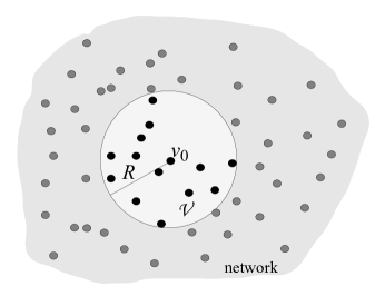
Figure 1: The set of valid nodes $\mathcal{V}$ is selected inside the disk of radius $R$ and origin the location of $v_{0}$.

The paper is organized as follows. In Section II, the model is described and some basic properties are given. In Section III, the main results for the case of grid-like networks are derived. Then in Section IV the case of randomly positioned networks is considered. A rate analysis is provided in Section V and simulation results are shown in Section VI. The paper is concluded in Section VII.

II Communication model

We assume a set of nodes $\mathcal{V}$, positioned on the plane. Communications between these nodes are established via the Boolean interference model (see, e.g., [7]). In this model, a link between two nodes $\{v_{i},v_{j}\}$ is realized if and only if $\left|\mathbf{X}(v_{i})-\mathbf{X}(v_{j})\right|\leq R$. In this case, we say that $v_{i}$ is connected with $v_{j}$ and vice versa. Note that the Boolean interference model is an undirected graph in the sense that only bi-directional links appear.

II-A Information flow

Each node $v_{i}$ having degree $\deg\left(v_{i}\right)>1$, apart from transmitting and receiving, relays information. In this process, it is possible to avoid unnecessary transmissions by employing local network coding. To simplify the analysis, we will consider only one cell, i.e., we will focus on a given node $v_{0}$, and all its neighbors, and calculate the network coding gain on the downlink of this node. A similar result, then, holds for any such node serving as a relay. Thus we restrict $\mathcal{V}$ to contain all neighbors of $v_{0}$, with $\mathcal{V}=\{v_{1},v_{2},\dots,v_{N}\}$ and $N\doteq\left|\mathcal{V}\right|$ the number of nodes under consideration. For a network determined by a Poisson point process with density $\lambda$, we use correspondingly the mean number of points which is given by $\mathrm{E}\!\left[N\right]=\lambda\pi R^{2}$. The main objective of this paper is to find how the maximum coding number and the maximum network coding gain scale with the number of nodes. Also we will provide bounds for the scaling constants which are useful for determining the behaviour in small networks.

Apart from the number of neighbors, the gain analysis depends also on the activated flows. In the simple Alice–relay–Bob topology, it is possible that only the flow going from Alice to Bob is activated, in which case the gain is zero. In this paper we are interested in determining an upper bound for the efficiency loss when the relay is constrained on combinations of size $m<N$ (e.g. if $m=2$ the system is constrained to pairwise XORing). For this reason, we consider the maximum gain scenario. For each node designated as a relay, we assume that all possible two–hop flows traversing this relay are activated. This means that each node designated as a relay, has all possible different packets from which to select an XOR combination to send to the neighbors. Since not all of those combinations are valid, finding the maximum valid combination that corresponds to the maximum coding number is a non-trivial task and will be the goal of this paper. The resulting bound will help characterize the efficiency loss due to resorting to $m$-wise encoding. In real systems, some flows might not be active in which case the resulting efficiency loss from $m$-wise encoding will be even smaller.

To make this more precise, similar to [17], we define source-destination pairs designating 2–hop flows that cross the relay. Each flow $f\in\mathcal{F}$ has a source $S(f)$, a destination $D(f)$, a set of nodes having it $H(f)\subset\mathcal{V}$ (either by overhearing or ownership) and a set of nodes needing it $N(f)\subset\mathcal{V}$. We write $\subset$ because at least one node, the destination $D(f)$ or the source $S(f)$, is not part of $H(f)$ and $N(f)$ correspondingly. Two flows $f_{1},f_{2}$ are called symmetric when they satisfy the property $S(f_{1})=D(f_{2})$ and $D(f_{1})=S(f_{2})$.

II-B Constraints

Here we summarize the previous subsection in the form of constraints. We will focus on network coding opportunities appearing in the aforementioned arbitrary network around the relay $v_{0}$.

Definition 1.

(valid node): A node $v_{i}\in\mathcal{V}$ is a valid node if $\left|\mathbf{X}(v_{i})-\mathbf{X}(v_{0})\right|\leq R$.

Definition 2.

(valid flow): A flow $f\in\mathcal{F}$ is a valid flow if $S(f)$ and $D(f)$ are valid nodes not neighboring with each other, i.e., $\left|\mathbf{X}(S(f))-\mathbf{X}(D(f))\right|>R$.

Definition 3.

(valid combination): A subet of flows $\mathcal{C}\subseteq\mathcal{F}$ with $\mathcal{C}=\{f_{1},f_{2},\dots,f_{C}\}$, where $C=\left|\mathcal{C}\right|$, is a valid combination if

• each flow $f_{i}\in\mathcal{C}$ is a valid flow,

• every pair of flows $f_{i},f_{j}\in\mathcal{C},f_{i}\neq f_{j}$ satisfies $N(f_{i})\subseteq H(f_{j})$ and $N(f_{j})\subseteq H(f_{i})$ or equivalently, $S(f_{i})$ is connected with $D(f_{j})$ while $S(f_{j})$ is connected with $D(f_{i})$.

We define the maximum coding number $C_{\max}$ as the greatest cardinality among all valid sets $\mathcal{C}$. If the positions of the network are random, $C_{\max}$ is evidently a random variable.

Note that we could impose additional constraints. For example, if a flow can be routed more efficiently by a node other than $v_{0}$, then this flow should be excluded from the set of valid flows. This would restrict further the set of valid combinations and thus by omitting this constraint we derive an upper bound for $C_{\max}$.

Next, we state some fundamental properties of the valid combinations. For each flow $f$ belonging to a valid combination $\mathcal{C}$ we have

• $D(f)\in N(f)$,

• $D(f)\in H(j)$ for all $j\in\mathcal{C}\setminus\{f\}$,

which leads us to the following properties.

Remark 1.

The destination node of $f_{i}\in\mathcal{C}$ is different from the destination node of any other flow $f_{j}\in\mathcal{C}\setminus\{f_{i}\}$.

Remark 2.

The source node of $f_{i}\in\mathcal{C}$ is different from the source node of any other flow $f_{j}\in\mathcal{C}\setminus\{f_{i}\}$.

Next, we provide a result on the topology for a valid combination. Let $\mathcal{X}_{\mathcal{C}}$ represent the set of locations of all nodes being the source or destination of a flow belonging to a combination $\mathcal{C}$.

Lemma 1.

Any valid combination of size 3 or larger corresponds to a convex polygon (the polygon is formed using the set $\mathcal{X}_{\mathcal{C}}$ as edges).

Proof.

Consider a valid combination defined by flows

$$\mathcal{C}=\left\{{f_{i},i=1,\ldots,C}\right\},$$

where $C\geq 3$. Consider also the set of nodes that are sources and/or destinations in $\mathcal{C}$

$$\mathcal{V}_{\mathcal{C}}=\cup_{i}S(f_{i})\cup_{i}D(f_{i})$$

and the induced set of locations $\mathcal{X}_{\mathcal{C}}$ such that we have a bijective mapping for each element $v_{j}\in\mathcal{V}_{\mathcal{C}}$ with an element $\mathbf{X}(v_{j})\in\mathcal{X}_{\mathcal{C}}$.

Assume that there is a node $v_{j}\in\mathcal{V}_{\mathcal{C}}$ which is an interior point of the convex hull of $\mathcal{X}_{\mathcal{C}}$. Thus its location $X_{j}=\mathbf{X}(v_{j})$ can be written as $X_{j}=\sum_{i\not=j}\alpha_{i}X_{i}$ where $\sum_{i\not=j}\alpha_{i}=1$ and $\alpha_{i}\geq 0$ for all $i$.

On the other hand, there is a unique $v_{j^{*}}\in V_{\mathcal{C}}$, which is the communicating pair (source or destination) of $v_{j}$ in at least one flow, so that

$$|X_{j}-X_{j^{*}}|>R.$$ (1)

All the other nodes (destinations or sources) in $\mathcal{V}_{\mathcal{C}}$ should be able to reach the node $v_{j^{*}}$ directly. Thus,

$$|X_{j}-X_{j^{*}}|\leq\sum_{i\not=j}\alpha_{i}|X_{i}-X_{j^{*}}|\leq\sum_{i\not=j}\alpha_{i}R\leq R,$$

which is a contradiction to (1). Consequently the node $v_{j}$, as well as all other nodes of the combination, necessarily lie on the perimeter of the convex hull. Thus, the nodes of a valid combination are the vertices of a convex polygon. ∎

When the set of sources is identical to the set of destinations, the combination consists of symmetric flows only and $C=2(\left|\mathcal{V^{\prime}}\right|-1)$, $\mathcal{V^{\prime}}\subseteq\mathcal{V}$.

In order to calculate an upper bound of the network coding combination size, it is enough to resort to the case of symmetric flows.

Lemma 2.

For any valid combination there exists at least one combination of the same or larger size that contains only symmetric flows.

Proof.

We will show that for any flow we can add the symmetric one without invalidating the combination as long as it is not already counted.

In a bipartite graph with all the nodes $\mathcal{V}$ on one side and the destinations of $\mathcal{C}$ on the other, consider a directional link $\ell_{f}$, between the source of flow $f$ and its destination, for each $f\in\mathcal{C}$. Note now that the nodes having out-degree one, i.e., the active sources in $\mathcal{C}$, may or may not be identical to one of the destination nodes. We can make a partition of the set of active sources by assigning those with the above property to the set $\mathcal{T}_{\textsl{sym}}$ and the rest to the complementary set $\overline{\mathcal{T}_{\textsl{sym}}}$. If $\overline{\mathcal{T}_{\textsl{sym}}}=\emptyset$, then the Lemma is proved since $\mathcal{C}$ is a valid combination with symmetric flows only. If not, then we can create a new combination $\mathcal{C}^{\prime}$ which has more flows than the original one using the following process. For each transmitter in $\overline{\mathcal{T}_{\textsl{sym}}}$, say $S(f_{i})$ the transmitter of flow $f_{i}$, add one extra flow $f_{i}^{\prime}$ with $S(f_{i}^{\prime})=D(f_{i})$ and $D(f_{i}^{\prime})=S(f_{i})$. This flow does not belong to $\mathcal{C}$ (because $S(f_{i})\in\overline{\mathcal{T}_{\textsl{sym}}}$) and it does not invalidate the combination due to the bidirectional properties of the model. Note that $f_{i}^{\prime}$ is a valid flow because $S(f_{i}^{\prime})$ cannot be connected to $D(f_{i}^{\prime})$ due to validity of $f_{i}$. Note also that $S(f_{i}^{\prime})$ is connected to $D(f)$ for all $f\in\mathcal{C}$ since this is again required for the decoding of the original flows. Thus, for any flow we can add the symmetric one without invalidating the combination. ∎

Remark 3.

If a valid combination consists of symmetric flows only, its size must be even.

In graph theory terms, a valid combination with symmetric flows can be thought of as a graph created by a clique of $C+1$ nodes, minus a matching with $\frac{C}{2}$ edges, with all symmetric flows defined by this matching activated. This graph is called in [11] wheel topology.

III Analysis in grid-like topologies

In this section we focus on positioning the nodes on a grid. Grid topologies often offer an insightful first step approach towards the random positioning behaviour. Also, the investigation of grids answers the question whether it is possible to achieve high NC gain by arranging the locations of the nodes.

We therefore assume a network with the additional property $\left|\mathbf{X}(v_{i})-\mathbf{X}(v_{j})\right|\geq d$, for any pair of nodes $v_{i},v_{j}\in\mathcal{V}$. This condition pertains to regular grids such as the square, the triangular and the hexagonal grid as well as other grids with non-uniform geometry. We impose nevertheless the property that the node density is the same over all cells and thus the geometry should be somehow homogeneous. The number of nodes inside a disk or radius $R$ will be $N=O\left((\frac{R}{d})^{2}\right)$ for these networks and the corresponding node density $\lambda^{\mathrm{grid}}=O\left((\frac{1}{d})^{2}\right)$.

Theorem 1.

(Upper bound) The maximum coding number in fixed-separation networks is $O\left(\sqrt{N}\right)$ where $N$ is the number of nodes or equivalently $O\left(\sqrt{\lambda^{\mathrm{grid}}}\right)$.

Proof.

From Lemma 1 we know that the nodes belonging to the maximum combination form a convex polygon. Any such polygon fitting inside the disk of radius $R$ must have perimeter smaller than $2\pi R$. Since the nodes on the perimeter should be at least $d$ away from each other, we conclude that the maximum coding number is

$$C_{\max}<\frac{2\pi R}{d}.$$

This combined with $N=O\left(\frac{R}{d}^{2}\right)$ or respectively $\lambda^{\mathrm{grid}}=O\left((\frac{1}{d})^{2}\right)$ yields the result. ∎

A particular case of the above bound is the square grid. The number of nodes inside the disk is $N=\pi\left(\frac{R}{d}\right)^{2}+e\left(\frac{R}{d}\right)$ where $e\left(\frac{R}{d}\right)\leq 2\sqrt{2}\pi\frac{R}{d}$ is an error decreasing linearly with $d$. Thus we obtain an upper bound

$$C_{\max}^{\textsl{square}}<\sqrt{4\pi N}.$$

So far we have shown that any network with fixed separation distance $d$ and uniform density, will have maximum coding number of $O(\sqrt{N})$, where $N$ is the number of nodes connected to the relay. In particular, the constant can be determined for any given grid and for the square grid is $2\sqrt{\pi}$. The simulations show that the actual maximum encoding number is approximately half of that calculated above. The reason for that is basically that the valid polygon is always smaller than the disk of radius $R$ and often close to the size of a disk of radius $\frac{R}{2}$.

It is interesting to bound the achievable maximum coding number from below as well. To obtain intuition about this bound we start with a non-homogeneous topology, the cyclic grid. We construct concentric cyclic groups of radius $R_{i}=id$, $i=0,1,\dots,\lfloor\frac{R}{d}\rfloor$ that fall inside the disk of radius $R$. Each cyclic group has as many nodes as possible such that the fixed separation distance condition is not violated. Such a topology exhibits different behavior depending on the selected origin (it is not homogeneous), nevertheless it helps identify a particular behavior of the achievable maximum coding number. The cyclic group at $R_{i}$ has $\left\lfloor\frac{2\pi}{\arccos\left(1-\frac{1}{2i^{2}}\right)}\right\rfloor$ nodes. Thus the grid of radius $R$ will have

$$N=1+\sum_{i=1}^{\left\lfloor\frac{R}{d}\right\rfloor}\left\lfloor\frac{2\pi}{\arccos\left(1-\frac{1}{2i^{2}}\right)}\right\rfloor.$$

A very good approximation is,

$$\begin{split}N&\approx 1+6\sum_{i=1}^{\left\lfloor\frac{R}{d}\right\rfloor}i\\ &=1+\left\lfloor\frac{R}{d}\right\rfloor+\left\lfloor\frac{R}{d}\right\rfloor^{2}\\ &\approx 3\frac{R^{2}}{d^{2}}.\end{split}$$ (2)

Theorem 2.

(Lower bound) In networks with nodes $d$ away from each other and cell radius $R$, an achievable maximum coding number is

1. $C_{\max}^{\textsl{cyclic}}=\Omega(\sqrt{N})$ for cyclic grid with $\mathrm{rem}\left(R,2d\right)\rightarrow 0$,

2. $C_{\max}^{\textsl{cyclic}}=\Omega(\sqrt[4]{N})$ for cyclic grid with $\mathrm{rem}\left(R,2d\right)\rightarrow d$ and

3. $C_{\max}^{\textsl{square}}=\Omega(\sqrt[4]{N})$ for the square grid of $d$,

where $\mathrm{rem}(x,y)$ is the remainder of the division $x/y$.

Proof.

For the cyclic grid when $\mathrm{rem}\left(R,2d\right)\rightarrow 0$: By focusing on the cyclic group with $\inf\{i:R_{i}>\frac{R}{2}\}$, note that each node is $\frac{R}{2}+\epsilon$ from the center and thus the desired connectivity properties are satisfied for all nodes on the cyclic group. In this case, we can calculate the number of nodes in the group as

$$C_{\max}^{\textsl{cyclic}}=\left\lfloor\frac{2\pi}{\arccos\left(1-\frac{2d^{2}}{R^{2}}\right)}\right\rfloor,$$

which for large $N$ is bounded from below by some linear function of $\sqrt{N}$.

For the cyclic grid when $\mathrm{rem}\left(R,2d\right)\rightarrow d$: Now each node is $\frac{R}{2}+d-\epsilon$ away from the center and thus we need to select those nodes satisfying the property of valid combination. For this it is enough that we leave an empty angle $\phi$ such that if $AOB$ is a diameter and $AOC$ this angle, then $CB\leq R$. By solving this for the maximum number of points satisfying this property we get

$$C_{\max}^{\textsl{cyclic}}=\left\lfloor\frac{2\pi}{\arccos\left(\frac{R^{2}}{2\left(\frac{R}{2}+d\right)^{2}}-1\right)}\right\rfloor,$$

which for large $N$ is bounded from below by some linear function of $\sqrt[4]{N}$.

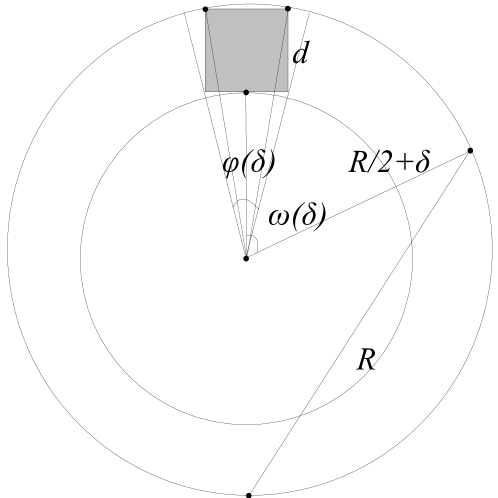
Figure 2: Sketch for the proof of Theorem 2.

For the square grid: we construct a ring around the circle of $\frac{R}{2}$ radius. The width of the ring is $\delta$ wide enough to fit a whole squre of dimensions $d\times d$. Such a square is bound to contain exactly one node of the grid. Using Figure 2, and the triangles relative to the small square, we calculate $\delta$ as

$$\delta=\frac{\sqrt{R^{2}+d(5d+4R)}-R}{2}.$$

Thus we can show that $d\leq\delta\leq\frac{3d}{2}$. If we use the largest possible value that guarantees that the ring contains one node at each step, namely $\delta=1.5d$, we can compute the angle that contains at least one node, which is of the order of $d$:

$$\phi(\delta)=\arcsin\left(\frac{\sqrt{2}d}{\sqrt{d^{2}+R^{2}}}\right).$$

Finally, we compute the angle which should be left empty in the valid combination such that any node outside this angle is reachable by the most distant node (the one at the bottom).

$$\omega(\delta)=\arcsin\left(\frac{R}{\sqrt{2}(R+1.5d)}\right).$$

This angle is of the order of $\sqrt{d}$. Finally an achievable combination is obtained if we alternate $\phi$ and $\omega$ until we fill the circle.

$$C_{\max}^{\textsl{square}}=\left\lfloor\frac{2\pi}{\phi(\delta)+\omega(\delta)}\right\rfloor,$$

which is bounded from below by a linear function of $\sqrt[4]{N}$. Note that the sparseness of the combination is due to $\omega(\delta)$ and a possible reasoning is that the bound is constructed to cover all the cases, thus also the case that the uncomfortable positioning of nodes matches the second case of the cyclic grid above. ∎

In [2], relative results on convex polygons in constrained sets guarantee the existence of convex polygons of size $\Omega(\sqrt[4]{N})$ when the $N$ thrown nodes are kept seperated by some distance.

IV Stochastic analysis

Assume that the locations of the nodes are determined by a Poisson point process with density $\lambda$. The connectivity properties of this model are well studied in the literature (see e.g. [15, 6]). In our work, we assume that the network is percolating, i.e. the nodes are dense enough to ensure multihop communications. As in the deterministic case, we assume that a relay is located at the origin. For a Poisson point process this assumption does not change the distribution of the other points. The main result is an upper bound in probability for the maximum coding number.

Theorem 3.

In a random network determined by a Poisson point process with density $\lambda$, the maximum coding number corresponding to combinations having the relay at the origin satisfies

$$\lim_{\lambda\to\infty}\mathrm{P}\!\left(C_{\max}(\lambda)=O(\lambda^{1/2+\epsilon})\right)=1,$$

for any $\epsilon>0$.

Proof.

Cover the disk of radius $R$ around the origin by disjoint boxes of size $\frac{1}{\sqrt{\lambda}}\times\frac{1}{\sqrt{\lambda}}$. The number of nodes inside the boxes is denoted by $N_{i}$, $i=1,\ldots,n(\lambda)$. The $N_{i}$ are identically and independently $\mathrm{Poisson}(1)$ distributed and thus there is a sequence $I_{n}$ such that

$$\lim_{n\to\infty}\mathrm{P}\!\left(\max_{1\leq i\leq n}N_{i}=\mbox{$I_{n}$ or $I_{n}+1$}\right)=1,$$

where $I_{n}=O\left(\frac{\log n}{\log\log n}\right)$ (see [3, 14]). Since $n(\lambda)=O(\lambda)$,

$$\lim_{\lambda\to\infty}\mathrm{P}\!\left(\max_{i=1,\ldots,n(\lambda)}N_{i}=O\left(\frac{\log\lambda}{\log\log\lambda}\right)\right)=1.$$ (3)

Next consider a valid combination. By Lemma 1, the nodes of the combination form a convex polygon. The perimeter of any convex polygon is at most $2\pi R$ because it is located inside the disk of radius $R$. Since at most $O(\sqrt{\lambda})$ boxes of size $\frac{1}{\sqrt{\lambda}}\times\frac{1}{\sqrt{\lambda}}$ are needed to cover the perimeter of any convex polygon,

$$C_{\max}(\lambda)\leq\max_{i=1,\ldots,n(\lambda)}N_{i}O(\sqrt{\lambda})\quad\mbox{a.s.}$$

This implies that

$$\mathrm{P}\!\left(C_{\max}(\lambda)\leq O(\sqrt{\lambda}g(\lambda))\right)\geq\mathrm{P}\!\left(\max_{i=1,\ldots,n(\lambda)}N_{i}\leq O\left(g(\lambda)\right)\right).$$

Setting $g(\lambda)=\log\lambda/\log\log\lambda$, applying equation (3) and finally noticing that $\log\lambda/\log\log\lambda=O\left(\lambda^{\epsilon}\right)$ for any $\epsilon>0$ completes the proof. ∎

V Rate efficiency of a network coding combination

We will focus on the downlink of a valid combination of size $C$. Without loss of generality, assume that the rate vector $\mathbf{r}=\{r_{i}\}_{i=1,2,\dots,C}$ is ordered, i.e., $r_{1}<r_{2}<\dots<r_{C}$, and that the flow set is permuted accordingly so that over the link $\left(v_{0},D(f_{i})\right)$ packets are transfered at a rate $r_{i}$.

The data rate is computed as the number of packets of size $P$ transmitted in a virtual frame over the time needed for these transmissions. Since an encoded packet is always transmitted at the lowest rate decodable by all receivers and assuming max-min fair allocation, we can deduce the maximum throughput rate with network coding as

$$r_{\textsl{NC}}(C)=\frac{CP}{\frac{P}{\min\{\mathbf{r}\}}}=Cr_{1}.$$

The rate without NC would be

$$r_{\textsl{w}}(C)=\frac{CP}{\frac{P}{r_{1}}+\frac{P}{r_{2}}+\dots+\frac{P}{r_{C}}}=C\left(\sum_{i=1}^{C}\frac{1}{r_{i}}\right)^{-1}=r_{h},$$

where $r_{h}$ is the harmonic mean of $\mathbf{r}$. Choosing any $m\leq C$ and allowing for combinations of size $m$ at most, it is easy to see that if the criteria for valid combinations are fulfilled for combination of size $C$ then they are fulfilled for all subsets. The corresponding achievable rate is

$$\begin{split}r_{m}(C)&=\frac{CP}{\sum_{i=1}^{\left\lfloor\frac{C}{m}\right\rfloor}\frac{P}{r_{m(i-1)+1}}+1_{\{\mathrm{rem}\left(C,m\right)>0\}}\frac{P}{r_{C-\mathrm{rem}(C,m)+1}}}\\ &=C\left(\sum_{i=1}^{\left\lfloor\frac{C}{m}\right\rfloor+1_{\{\mathrm{rem}\left(C,m\right)>0\}}}\frac{1}{r_{m(i-1)+1}}\right)^{-1},\end{split}$$

Next, we derive the network coding gain for the maximum combination ($C$) and for the constrained group ($m\leq C$).

$$g(C)\doteq\frac{r_{\textsl{NC}}(C)}{r_{\textsl{w}}(C)}=C\frac{r_{1}}{r_{h}}.$$

Note that the gain is a linear function of $C$ and depends on the particularities of the rate vector. Also,

$$\begin{split}g_{m}(C)&\doteq\frac{r_{m}(C)}{r_{\textsl{w}}(C)}=\\ &=\frac{C}{r_{h}}\left(\sum_{i=1}^{\left\lfloor\frac{C}{m}\right\rfloor+1_{\{\mathrm{rem}\left(C,m\right)>0\}}}\frac{1}{r_{m(i-1)+1}}\right)^{-1}\\ &\geq\frac{C}{r_{h}}\left(\frac{\left\lceil\frac{C}{m}\right\rceil}{r_{1}}\right)^{-1}\geq(m-1)\frac{r_{1}}{r_{h}},\end{split}$$

where in the first inequality we have used that $r_{1}$ is the minimum rate, and in the second we have used $m-1\leq\frac{C}{\left\lceil\frac{C}{m}\right\rceil}\leq m$. If we choose equal rates, then we readily get $g(C)=C$ and $\max\left\{g_{m}(C)\right\}=m$ as the maximum gain for both. Finally we can symbolize that $g(C)=\Theta(C)$ and moreover the difference $g(C)-g_{m}(C)=O(C-m)$. Therefore, the efficiency loss is of the order of $\sqrt{N}-m$ which means that for carefully chosen $m$, the loss can be kept small.

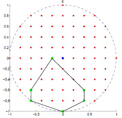
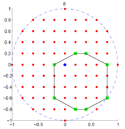
Figure 3: Coding combination examples for $C_{\max}=6$ and $C_{\max}=8$ in a square grid with $N=81$.

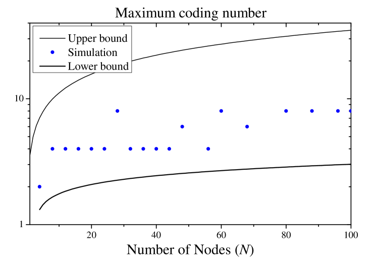
Figure 4: Simulation of maximum coding number of a square grid inside a disk with $N$ nodes. $C_{\max}$ is the upper bound and $C_{\min}$ is the achievable lower bound provided in the theoretical analysis.

VI Numerical results

In this section we present some simulation results that provide further evidence and insight for our work. For simulation purposes we consider a disk of radius $R=1$ and a node $v_{0}$ serving as a relay situated at the center of the disk. Initially we consider a square grid of nodes over this disk and we investigate the maximum coding number, i.e., a set of nodes that satisfies the constraints of section II. Then, the scenario of uniformly random thrown nodes is considered.

VI-A Experiments with square grids

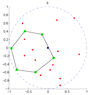
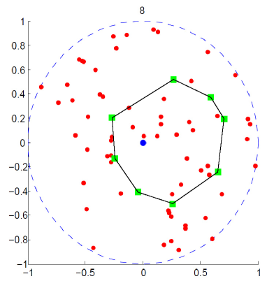
Figure 5: Maximum coding combination examples for $C_{\max}=6$ and $C_{\max}=8$ in a uniformly thrown network with $N=21$ and $N=70$ respectively.

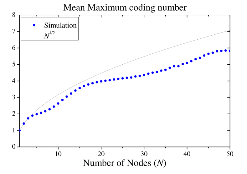
Figure 6: Mean maximum coding number in a network of $N$ uniformly thrown nodes.

Figure 3 showcases examples of combination size $C=6$ and $C=8$ (the maximum is $8$ in this case). During these experiments we identified an interesting property. We noticed that the maximum coding number depends only on the number of nodes inside the disk and not on the actual $d$ used. In particular, for all $\{d:N\text{ is fixed}\}$, $C_{\max}$ is constant. In Figure 4 we present the results for the square grid. The actual values seem to be closer to the lower bound than to the upper, leading to an order closer to $\sqrt[4]{N}$ (notice the logarithmic scale of the figure). Nevertheless, the oscillating effect due to the interplay between the radius and the number of nodes is evident.

VI-B Experiments with randomly positioned nodes

Next, we throw $N$ nodes uniformly inside the disk of radius $R=1$. Examples of maximum coding number are showcased in Figure 5. It is noted from these examples that large combinations tend to appear in a $\delta$–ring form where the inner side of the ring is a disk of radius $\frac{R}{2}$ and the outer side is a disk of radius $\frac{R}{2}+\delta$.

In Figure 6, we present the mean maximum coding number, for different number of nodes $N$. In each sample, the maximum coding number is calculated and the mean is obtained by averaging over $1000$ random samples. The $O(\sqrt{N})$ behavior is depicted in this picture.

Figure 7 shows the probability of existence of at least one coding combination of size $C$ in a network of $N$ uniformly thrown nodes. For example, the maximum component size for $20\leq N\leq 50$ is either 4 or 6 in the majority of cases. The simulation results show that in real networks of moderate size the usual combination size is quite small. The multiplicative constant seems to be close to 1. In this context, the focus should be on developing efficient algorithms that opportunistically exploit local network coding over a wide span of topologies using small XOR combinations rather than attempting to solve complex combinatorial problems in order to find the best combinations available.

Figure 7: Probability of existence of at least one coding combination of size $C$ in a network of $N$ uniformly thrown nodes.

VI-C A realistic scenario

Next, we set up a realistic experiment to be run in simulation environment. A relay node is positioned at the origin, willing to forward any traffic required and apply NC if beneficial. Then, we throw $\frac{N}{2}$ pairs of nodes randomly inside the disk defined by the relay and the communication distance $R$; note that all nodes are valid nodes. Each pair constitutes a symmetric flow. Each flow may be valid or invalid depending on the distance between the two nodes, see definition in section II. Whenever the flow is invalid, the nodes communicate directly by exchanging two packets over two slots (one for each direction). If the flow is valid, the relay is utilized to form a 2-hop linear network. Again, 2 packets are uploaded towards the relay using two slots while the downlink part is left for the end of the frame. Finally, the relay has collected a number of packets which may be combined in several ways using NC. To identify the minimum number of slots required to transmit those packets to the intended receivers, we solve the problem of minimum clique partition with the constraint of using cliques of size up to $\frac{m}{2}$ (equivalently, combining up to $m$ packets together). In the above we have assumed that all links have equal transmission rates and that the arrival rates of the flows are all equal (symmetric fair point of operation). The network coding gain is calculated by dividing the number of slots used without NC by the number of slots using NC.

Figure 8 depicts results from simulated random experiments. Evidently, it is enough to combine up to two packets per time in order to enjoy approximately the maximum NC gain. This example supports the intuition that in practice the network coding gain from large combinations is expected to be negligible.

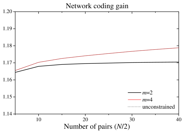
Figure 8: A realistic scenario. Pairs of nodes forming flows are randomly thrown inside the disk $(0,r)$. The relay node (situated at the origin) assists the flows that cannot communicate directly. We restrict NC combinations to size $m$ where $m=2,4,\infty$.

VII Conclusion

By considering the Boolean connectivity model and applying the basic properties required for correct decoding, we showed that for the local network coding there are certain geometric constraints bounding the maximum number of packets that can be encoded together. Particularly, due to the convexity of any valid combination, the sizes of combinations are at most order of $\sqrt{N}$ for all studied network topologies.

The fact that the number of packets is limited gives rise to approximate algorithms for local coding. Instead of attempting to solve the hard problem of calculating all possible coding combinations, we showed that an algorithm considering smaller combinations does not lose too much.

References

- [1] E. Ahmed, A. Eryilmaz, M. Medard, and A.E. Ozdaglar. On the scaling law of network coding gains in wireless networks. In proceedings of IEEE Military Communications Conference,MILCOM, pages 1–7, 2007.
- [2] N. Alon, M. Katchalski, and W. R. Pulleyblank. The maximum size of a convex polygon in a restricted set of points in the plane. Discrete Comput. Geom., 4(3):245–251, 1989.
- [3] C. W. Anderson. Extreme value theory for a class of discrete distributions with applications to some stochastic processes. Journal of Applied Probability, 7:99–113, 1970.
- [4] P. Chaporkar and A. Proutiere. Adaptive Network Coding and Scheduling for Maximizing Throughput in Wireless Networks. In ACM MOBICOM, 2007.
- [5] M. A. R. Chaudhry and A. Sprintson. Efficient algorithms for index coding. In proceedings of IEEE 27th Conference on Computer Communications (INFOCOM), 2008.
- [6] O. Dousse, P. Thiran, and M. Hassler. Connectivity in ad hoc and hybrid networks. In Proceedings of IEEE Infocom 2002. IEEE Computer Society, 2002.
- [7] M. Franceschetti and R. Meester. Random Networks for Communication: From statistical Physics to Information Systems. Cambridge University Press.
- [8] A. Goel and S. Khanna. On the network coding advantage for wireless multicast in euclidean space. pages 64–69, apr. 2008.
- [9] L. Jilin, J.C.S. Lui, and M.C. Dah. How many packets can we encode? - an analysis of practical wireless network coding. In IEEE INFOCOM 2008. The 27th Conference on Computer Communications, pages 371–375, apr 2008.
- [10] L. Junning, D. Goeckel, and D. Towsley. Bounds on the gain of network coding and broadcasting in wireless networks. In proceedings of IEEE INFOCOM, pages 724–732, 2007.
- [11] S. Katti, H. Rahul, W. Hu, D. Katabi, M. Medard, and J. Crowcroft. XORs in The Air: Practical Wireless Network Coding. In ACM SIGCOMM, 2006.
- [12] A. Keshavarz-Haddadt, , and R. Riedi. Bounds on the benefit of network coding: Throughput and energy saving in wireless networks. In proceedings of IEEE INFOCOM, pages 376–384, 2008.
- [13] Y. Kim and G. De Veciana. Is rate adaptation beneficial for inter-session network coding? Selected Areas in Communications, IEEE Journal on, 27(5):635–646, jun. 2009.
- [14] A.C. Kimber. A note on poisson maxima. Probability Theory and Related Fields, 63(4):551–552, 1983.
- [15] R. Meester and R. Roy. Continuum Percolation. Cambridge University Press.
- [16] S. Rayanchu, S. Sen, J. Wu, S. Banerjee, and S. Sengupta. Loss-Aware Network Coding for Unicast Wireless Sessions: Design, Implementation, and Performance Evaluation. In ACM SIGMETRICS, 2008.
- [17] E. Rozner, A. P. Iyer, Y. Mehta, L. Qiu, and M. Jafry. ER: Efficient Retransmission Scheme for Wireless LANs. In ACM CONEXT, 2007.
- [18] T. Wang and G. B. Giannakis. Capacity scaling of wireless networks with complex field network coding. Acoustics, Speech, and Signal Processing, IEEE International Conference on, 0:2425–2428, 2009.