Back To The Future: On Predicting User Uptime

Abstract

Correlation in user connectivity patterns is generally considered a problem for system designers, since it results in peaks of demand and also in the scarcity of resources for peer-to-peer applications. The other side of the coin is that these connectivity patterns are often predictable and that, to some extent, they can be dealt with proactively.

In this work, we build predictors aiming to determine the probability that any given user will be online at any given time in the future. We evaluate the quality of these predictors on various large traces from instant messaging and file sharing applications.

We also illustrate how availability prediction can be applied to enhance the behavior of peer-to-peer applications: we show through simulation how data availability is substantially increased in a distributed hash table simply by adjusting data placement policies according to peer availability prediction and without requiring any additional storage from any peer.

1 Introduction

User uptime patterns in Internet applications are known to be very different from what would be obtained from random, uncorrelated models. Many measurements [3, 1, 10, 5, 11, 6] confirmed that traces of different applications have daily and weekly patterns. User uptime therefore cannot be modeled as a simple Markovian process, because user activity is often correlated.

In system design, correlation is often seen as a problem: for instance, simultaneous requests from many users results in a “flash-crowd” phenomenon which is problematic for content distribution systems; in peer-to-peer storage systems, the fact that many user are offline at the same time creates problems with respect to data availability.

In this work, we strive to build a set of predictors to exploit the correlated nature of user activity. Indeed, if users do not behave randomly, then it should be possible to design mechanisms capable of anticipating user behavior with a certain degree of precision.

A considerable amount of effort has been devoted to characterizing and predicting session lengths and future uptime patterns within a short time span [10, 13, 5, 11, 7]; however, long-term predictions have been largely neglected, and the probability for a user to be online is generally modeled as the same for each user and each moment in the future.

In [10], which is the closest to our work, uptime predictors are built around the concept of saturating counters and refinements thereof, and go beyond a boolean classification of user online time. However, such techniques are not easily amenable to anticipate the long term user behavior and do not account for users that abandon an application.

In this work, we build refined mechanisms for predicting long-term user behavior that also account for user departures. We verify the quality of our techniques on traces of Internet applications such as instant messaging and peer-to-peer applications, and we show that elaborate predictors are able to consistently reduce the uncertainty about future user behavior.

Our techniques can be used in many cases where individual user behavior has an influence on application performance like for example social networks or peer-to-peer storage applications. To illustrate the benefits derived from using the information provided by our predictors, we simulate a distributed hash table (DHT) and show that an informed policy for choosing node identifiers can result in higher data availability without requiring additional storage resources from nodes nor major modifications to the base DHT mechanism.

2 Datasets

In the context of Internet applications, a user generally launches an application (e.g., a P2P client), establishes a connection to other users or to a server, and finally disconnects from the service. We term this series of actions the user’s online behavior. The online behavior is used to compute the user availability, defined as the cumulative amount of time spent online, in a reference period of 24 hours.

We analyzed a variety of application traces to study the online behavior of users and to compute user availability distributions. We considered an instant messaging application (labelled IM in the following), the eMule file-sharing application relying on the Kad network [9] (labelled Kad) and the Skype VoIP application (labelled Skype). For IM, an author of this work is one of the administrators of a large IM service in Italy and had access to server logs indicating the online behavior of users. For Kad, we used the traces collected in [11] and for Skype, we used the dataset from [5], obtained by crawling the Skype super-peer network and made available on [8]. Table 1 summarizes the salient features of the three datasets: the trace duration ranges from roughly 1 to 6 months and the number of captured users ranges from roughly 2000 up to several hundred thousand users.

Trace	Duration	Users	High availability ($\geq 0.17$)
IM	172 days	1,825	354 (19.4%)
Kad	179 days	400,375	10,279 (2.57%)
Skype	24 days	2,081	1,174 (56.52%)

Table 1: Basic dataset information.

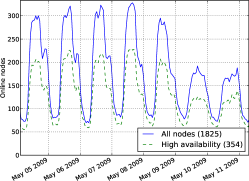
(a) IM.

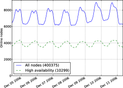
(b) Kad.

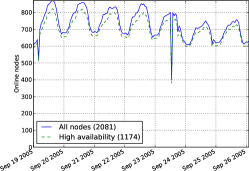
(c) Skype.

Figure 1: Number of online users in an arbitrary week of our different datasets.

What information do the above traces convey regarding the online behavior of users? Fig. 1 illustrates, for an arbitrary week of each datasets, the number of online users per day, detailing users with an availability larger than an average of four hours per day. The user behavior is highly correlated: hourly, daily, and weekly patterns clearly arise. Furthermore, we can pinpoint at important differences of such patterns depending on the application examined. In the IM trace, the online behavior is affected by weekends: in the last two days of the week displayed in Fig. 1a, a considerable fraction of users remained offline. In contrast, the Kad trace indicates a stable online behavior over a week: users connect mostly at night, which is particularly true for highly available users. Clearly, a regularity in the aggregate traces does not however imply that individual user behavior is regular. Lastly, in the Skype trace one can notice that most of the online users are highly available: this is a result of the crawling methodology used in [5] which only collects traces of super-peers. Some visible measurement artifacts are due to network problems on the measurement site.

The cumulative distribution of user availability is also clearly distinct for every application trace, as shown in Fig. 2. Indeed, user availability derives from the online behavior, as a result of implicit or explicit incentive mechanisms.

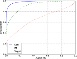
Figure 2: CDF of user availability.

For the IM application, incentives for users to stay online are implicit and intrinsic to the application itself. Indeed, IM applications are synchronous, although tolerant to delays, and require parties to be online at the same time to communicate. The CDF of user availability (Fig. 2) indicates that a large fraction of the users are sporadically online, and a small fraction of users have an availability larger than 0.4.

For the Kad application, incentives for users to stay online are explicit. Kad is used to support eMule, a file-sharing application, which implements a quite elaborate incentive mechanism that prioritizes users with a high availability when awarding upload slots [2]. The CDF of user availability is even more skewed (Fig. 2), indicating that a very large fraction of users are rarely available, while a tiny set of users have an availability larger than 0.2.

Finally, for the Skype application, incentives are implicit. VoIP applications are not delay tolerant and users need to be online to be reached by others. The distribution of user availability is more uniform than in the other cases (Fig. 2), apart from an appreciably small fraction of users that are not available.

As clearly highlighted above, the user behavior is a combination of personal factors, like for instance the user’s willingness to remain online or user time zone, and external factors, like application specific incentives or connectivity between hosts. Given the variety of resulting behaviors, the question we try and address in the following is whether simple predictors of the future availability of a user can be designed and tuned, and whether their prediction accuracy is influenced by the very nature of the application itself.

Before describing the details of our prediction techniques, some further observations have to be drawn. Any attempt at anticipating the online behavior of users would be doomed to introduce errors if the eventuality for a user to abandon indefinitely an application was omitted. For this reason, we analyzed the user mortality rate in our traces, defined as the rate of users “disappearing” from a dataset.

As a second observation, even though most related work focused on continuous availability estimates, correlated behaviors seem to be the most critical parameter that needs to be estimated. However, such correlated behaviors lead to the need for sophisticated predictors tailored to users rather than attempting to be generic. In Fig. 3, we focus on the IM and Kad traces and rearrange them by applying an off-the-shelf clustering algorithm ($k$-means). We arbitrarily define $k=6$ clusters (labelled $C_{i}$ in the figure) and plot the percentage of online users per cluster. It can be observed that there are two classes of peers (the first and the last cluster) that comprise a non-negligible fraction of the total user population, for which user availability is very high and very low, respectively. For such users, predicting their availability is simple. Instead, a large fraction of the user population exhibits very specific traits. For example, in Fig. 3a, users in $C_{1}$ have a regular online behavior that is marginally affected by a particular day of the week, while users in $C_{2}$ are highly influenced by weekends, i.e., the last two days displayed in the plot. Fig. 3b illustrates another kind of user-specific behavior: each cluster groups users with consistently distinct availability figures.

Both observations support our claim that the design of prediction algorithms, and in particular the tuning phase, should be tailored to the specific traits of a particular user. An evaluation of the accuracy of general predictors versus that obtained by individual predictors is provided in Sec. 4. The predictors described in the following are also adjusted to account for permanent user departures.

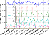
(a) IM.

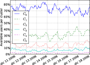
(b) Kad.

Figure 3: Clustered traces: detail of single weeks.

3 Prediction Algorithms

To describe the long-term behavior of users, our prediction algorithms face the task of anticipating, based on a history of past actions, the probability $p_{i,t}$ that a user $i$ will be online at any time $t$ in the future. To do so, we divide our traces between a training period from which past observations are drawn and a test period in which predictions are evaluated.

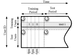
Figure 4: Chopping the traces: an illustrative example of our four-step approach.

Since tuning a handful of parameters was required to make our algorithms work properly, we adopted a four-step approach to the evaluation, as exemplified in Fig. 4. Besides dividing traces between a training and a test period, we distinguished between the nodes used to “train” the algorithm and those used to validate it. Predictors are first trained on the first quadrant; in the “fitting” phase, predictors are tuned to provide optimal performance on the training users for the test period (second quadrant). In the third phase the predictors, now properly tuned, get trained with the test users in the training period, and their accuracy is evaluated on the test periods in the fourth phase. In a real situation with growing traces, tuning would naturally be a dynamic process that would be re-evaluated as the mass of available information grows.

In the following, we use Mean Squared Error (MSE) as a metric to assess prediction accuracy, considering the prediction error as $\left(1-p_{i,t}\right)^{2}$ if user $i$ is actually observed online at time $t$, and $\left(p_{i,t}\right)^{2}$ if $i$ is instead offline. A “completely uninformed” predictor always predicting $p_{i,t}=0.5$ for any $i$ and $t$ would obtain a MSE of 0.25. The MSE exhibits a key property (as opposed to other metrics such as, for example, Mean Absolute Error): if an event has probability $\overline{p}$, the prediction $p$ that minimizes the MSE is exactly $p=\overline{p}$. Indeed, the expected MSE is $\overline{p}\left(1-p\right)^{2}+\left(1-\overline{p}\right)p^{2}=p^{2}-2p\overline{p}+\overline{p}$, whose differentiation leads to $2\left(p-\overline{p}\right)$. The function is therefore minimized when $p=\overline{p}$.

We now describe a range of algorithms that differ in the way the history of past user behavior is processed. For simplicity, we use Fig. 4 and illustrate the first training phase described above. The input to our algorithms is a matrix, where rows are user identifiers and columns correspond to a moment identified by time and day of week (e.g., monday, 6PM). The difference in time between columns is a tunable parameter (1 hour in the example). Each cell contains a value indicating the time ratio a user was online at that particular time during the training period. Fig. 4 provides example values for user $i$.

In the Flat predictor, we compute the average user availability for all users and all time-slots, i.e., using the entire matrix described above. Hence, $p_{i,t}$ equals the average user availability for all future time instants. A more refined approach takes into account weekly patterns. In the Weekly periodic predictor, $p_{i,t}$ is the average availability of all users for a reference day and time of the week, that is $p_{i,t}$ is computed for the column identified by the day of week and hour of $t$. For example, if $t$ corresponds to 6PM on a Monday, $p_{n,t}$ is the average availability for every Monday at 6PM in the training period. The Daily periodic predictor focuses on daily patterns: hence, $p_{i,t}$ is the average availability of all users for a reference time of the day, that is $p_{i,t}$ is computed for all the columns identified by the hour of $t$, irrespectively of the day of the week. As users exhibit very different behavior during the week and during weekends, as illustrated in Fig. 3, we designed a Weekend-aware daily periodic predictor, which isolates weekends from weekdays. This means that predictions in weekends (resp. weekdays) are only influenced by observations in weekends (resp. ordinary workdays).

Each approach elaborated above is implemented in two different “flavors”. A global version computes the statistic on all users, resulting in the same value of $p_{i,t}$ for each user; an individual variant only uses the behavior of user $i$ in the training period to compute $p_{i,t}$.

Moreover, we enhance the quality of prediction of all our approaches as follows (fitting step). First, we encode the possibility for users to leave indefinitely the system. We compute the user mortality rate $r$, as defined in Section 2, on the training users, and we update our original prediction to output $p^{\prime}_{n,t}=p_{n,t}\cdot r^{t}$: in our traces, we observed that highly available users quit an application with a roughly uniform probability. Secondly, we compute a linear regression such that the choice of $a$ and $b$ minimizes the MSE of $p^{\prime\prime}_{n,t}=ap^{\prime}_{n,t}+b$ on the training users, justified by the fact that we in general expect linear correlation between $p^{\prime}_{n,t}$ and the actual observations. We then use $p^{\prime\prime}_{n,t}$ adjusted with the new values of $r$, $a$, and $b$ as our predictor in the evaluation step.

Note that each of the predictors described so far specializes in capturing only a single trend of user behavior. A better predictor can take into account all these factors in order to output a more refined prediction. Our take at this task is a linear combination of all the previously defined predictors $p[i]$ (before linear correction): the resulting predictor is ${\hat{p}}_{n,t}=\sum_{i}c_{i}p[i]_{n,t}$, where the $c_{i}$ values are obtained via least-square fitting in order to minimize errors on the training users. We call this predictor ad-hoc, since the values of $c_{i}$ are different for each dataset and synthesize the regularities in the trace at hand.

4 Prediction Accuracy

In this section, we study the impact of the training period length on the accuracy of our predictors in terms of MSE. Both the IM and Kad traces are roughly 6 months long: we use the first three months of the trace as a candidate training period, while the test period begins on the first day of the fourth month. We therefore considered week, month, and three month long training periods, going backwards in time from the beginning of the test period (refer to Fig. 4).

For the accuracy analysis we filtered all users with an availability less or equal to 0.17 in the training period: indeed, those are the users whose behavior is the easiest to predict. Additionally, for the Kad dataset, we performed a random sampling of the user population and restricted our attention to 10,000 training users and 10,000 test users. The Skype trace is shorter than the other two traces: as a consequence, we only consider a week-long training period.

Dataset	Training period	Flat		Weekly		Daily		“Weekend”		Combined
		Global	Ind.	Global	Ind.	Glob.	Ind.	Glob.	Ind.	ad-hoc
	1 week	.2037	.1849	.2036	.1987	.2037	.1951	.2034	.1767	.1727
IM	1 month	.2039	.1770	.2036	.1936	.2037	.1912	.2032	.1657	.1601
	3 months	.2169	.1732	.2038	.1933	.2037	.1877	.2032	.1517	.1478
	1 week	.1780	.1638	.1783	.1699	.1779	.1612	.1779	.1632	.1608
Kad	1 month	.1778	.1636	.1778	.1666	.1777	.1605	.1777	.1615	.1598
	3 months	.1779	.1707	.1780	.1697	.1779	.1664	.1779	.1671	.1662
Skype	1 week	.2491	.2054	.2489	.2259	.2481	.1971	.2480	.2054	.1955

Table 2: MSE for the various basic predictors (lower is better).

Table 2 summarizes the MSE errors for the various predictors we designed in this work. We report measures for different training period lengths, as well as for the ad-hoc predictor, which combines the features of all preceding mechanisms. It should be mentioned that comparing the prediction accuracy across the three dataset reported in this table is somehow irrelevant. For example, the behavior of Skype users is more difficult to predict than the others, as the average availability is roughly 0.5. Hence, it is generally difficult to do better than an uninformed guess of $p_{n,t}=0.5$ that yields a MSE of 0.25. Instead, the prediction quality should be observed within a single dataset, comparing the various predictors to the Flat predictor.

As a general observation that applies to all our results, it appears that individual predictors perform better than global ones, which confirms the intuition that users are characterized by specific traits, as discussed in Sec. 2. Considering node mortality also ensures consistently better predictions, especially for the Kad dataset, where user mortality is higher.

Another global trend that can be observed from Table 2 is that prediction accuracy is related to the intrinsic nature of the datasets we study. For the IM dataset, which involves users connecting also from work, considering “specialized” predictors that include week days and weekends improves the prediction accuracy. In comparison, for the Kad dataset, users largely connect from home and at night and their behavior is not influenced by weekends. Thus, “specialized” predictors are not necessarily more accurate.

Finally, the ad-hoc predictor outperforms all other mechanisms we have designed, confirming that incorporating a range of periodic patterns effectively increases the prediction quality.

We now discuss the impact of the length of the training period on prediction accuracy. Global predictors are largely insensitive to training period lengths: one week of observations on user behavior appears to be sufficient to reach a plateau for MSE values. Instead, the individual and ad-hoc predictors are affected by the length of the history of past user behavior. In general, one could think that a longer training period would mitigate the “noise” introduced by a small number of samples on which the predictors are tuned. However, user behavior can also evolve with time, and as a consequence, the training phase used to tune our predictors might use obsolete data.

These observations are verified in our traces. As the rows corresponding to the IM trace in Table 2 show, longer training periods imply better accuracy, i.e., lower MSE values. Indeed, the behavior of the users of an IM application is regular on the long term. The Kad dataset exhibits an inverted trend: a longer training period entails lower prediction accuracy. Since the online behavior of Kad users evolves with time, shorter training periods are better to reflect these dynamics.

Overall, our results indicate that when properly tuned, our predictors can effectively anticipate user behavior, as confirmed by the low MSE values obtained. It is of course legitimate to question the concrete meaning of low MSE values. In particular, what is an acceptable level of accuracy? Obviously, it is impossible to design a predictor which makes no errors, and it is easy to define MSE=0.25 as an upper bound for the prediction error. We try and address this question in the following, where we study the impact of prediction accuracy in practice, our predictors being used to optimize the performance of an example application.

5 An Application Example

DHT applications are generic infrastructures mapping straightforwardly to the traces we have at hand as they can be used in both IM as well as file-sharing applications (as in the case of Kad). Here, we consider a Chord-like [12] DHT providing a key-value lookup primitive.

In our DHT model, identifiers and hash values for keys are distributed on a logical ring, and each information is replicated on a neighbor set of $n$ nodes whose identifiers are the closest successors to the hash of the key in the ring. We assume that information is stored on a long-term basis, so the data does not get erased from nodes between sessions: hence, data maintenance is required only when peers abandon the system for good. For simplicity, we do not implement maintenance mechanisms: data redundancy decreases with peer “death”.

In contrast to approaches that reduce object copying in a DHT by biasing replicas towards highly available nodes [10], we focus on improving data availability without imposing additional storage burden on any peer.

In general, node identifiers in DHTs are chosen via a random or pseudo-random function. We propose instead the application of a smart policy that maximizes data availability, i.e., the probability that at least one peer in each neighbor set will be online at any moment in the future. For example, a smart replica placement policy would distribute pieces of data between peers which are frequently online at day and at night in order to obtain high data availability.

The predicted availability of data placed in the DHT can be computed using the ad-hoc predictor for a neighbor set $N$ and a set of samples in time $T$ as

$$1-\frac{\sum_{t\in T}1-\prod_{n\in N}(1-p_{n,t})}{|T|}.$$

Since our predictors have a weekly period, we limit our analysis to the first week after the training period, sampling with a frequency of one hour.

Our optimizing algorithm works iteratively by repeatedly considering a pair of random nodes and verifying whether exchanging their identifiers would enhance, on average, the predicted data availability for the involved neighbor sets. If so, their identifiers get exchanged. The algorithm proceeds until swapping operations do not improve data availability over a fixed threshold. Although centralized in our simulations, this strategy can easily be implemented in a distributed fashion.

We executed our DHT simulation on the IM and Kad traces with a training period of 1 month, and on Skype with a training period of 1 week. All results are averaged on 10 simulation runs. Here we compute the replication factor $n$ using the traditional approach where user uptime is assumed to be uncorrelated. That is, we used the smallest $n$ that satisfies $1-(1-\overline{a})^{n}\geq 0.99$, where $\overline{a}$ is the average availability observed in the training period. Applying this formula resulted in a value of $n=15$ for Kad, $n=11$ for IM, and $n=5$ for Skype. Obviously, our predictions obtain different values for the estimated data availability, since in reality user behavior is strongly correlated.

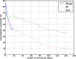
Figure 5: DHT simulation: benefits vs. test period.

The simulated data availability was computed by sampling the available nodes in the test period with a granularity of one hour, then computing the ratio of neighbor sets with at least one online node. The overall data availability was finally obtained by considering different lengths for the test period. For example, when a month is used as a training period, the average simulated data availability grows in IM from 0.95 to 0.98.

Data availability using the optimized ID allocation is consistently better than with a random placement. In Fig. 5 we show the benefits of the optimized ID allocation in terms of reduced data unavailability. For example, a 50% unavailability reduction means that the probability that a piece of data is unavailable is halved in the optimized case with respect to the original random allocation. As the test period grows, the benefits of the smart allocation policy decrease, both because some peers leave the system and because others change their behavior. In a real system, periodic data maintenance and identifier reallocation can be used to maintain good performances.

6 Conclusions

In this work, we studied the online behavior of users for a range of Internet applications. We designed and implemented simple predictors that anticipate user behavior capturing individual, global, daily, and weekly patterns. We evaluated the accuracy of our mechanisms and studied their impact on a “toy” DHT application, showing that user behaviors are predictable, which can be used to achieve considerable benefits in terms of data availability.

We believe that our work can be continued in various interesting directions. First, better predictors can be designed and tested, in particular on longer traces once they are available. While there is obviously an inherent level of unpredictability in the future behavior of users and even the smartest possible predictor will have a considerable margin of error, we are at the moment unable to guess if it is possible to obtain results that are substantially better than the ones that we are presenting here.

The DHT application that we presented in Section 5 is admittedly only a proof of concept. The task of incorporating our techniques into a real system will incur various tradeoffs, considering issues such as the cost of running the optimization algorithm and performing node repositioning. Also, security issues will need to be examined: could a malicious node be able to exploit such a repositioning protocol in order to disrupt the system?

Using our predictors to improve data placement in current P2P storage applications is an important objective. Additionally, we will explore other applications where availability predictions can be exploited. We believe that the knowledge of which users will be more likely to connect at a given moment in time could benefit social networking applications, e.g., to optimize pre-fetching schemes for home pages of users which are most likely to connect.

References

- [1] Ranjita Bhagwan, Stefan Savage, and Geoffrey Voelker. Understanding availability. In Peer-to-Peer Systems II, pages 256–267, 2003.
- [2] Luca Caviglione, Cristiano Cervellera, Franco Davoli, and Filippo Aldo Grassia. Optimization of an emule-like modifier strategy. Computer Communications, 31(16):3876 – 3882, 2008. Performance Evaluation of Communication Networks (SPECTS 2007).
- [3] Jacky Chu, Kevin Labonte, and Brian N. Levine. Availability and locality measurements of peer-to-peer file systems. In Proc. of ITCom: Scalability and Traffic Control in IP Networks, 2002.
- [4] D. Grolimund. Wuala - a distributed file system. Google TechTalks video, http://www.youtube.com/watch?v=3xKZ4KGkQY8, 2007.
- [5] Saikat Guha, Neil Daswani, and Ravi Jain. An experimental study of the skype peer-to-peer voip system. In Proc. IPTPS, 2006.
- [6] Bahman Javadi, Derrick Kondo, Jean M. Vincent, and David P. Anderson. Mining for Availability Models in Large-Scale Distributed Systems:A Case Study of SETI@home. In MASCOTS 2009. IEEE, September 2009.
- [7] D. Kondo, A. Andrzejak, and D. P. Anderson. On correlated availability in internet-distributed systems. In Proceedings of the 2008 9th IEEE/ACM International Conference on Grid Computing, pages 276–283. IEEE Computer Society, 2008.
- [8] D. Kondo, B. Javadi, A. Iosup, and D. Epema. The failure trace archive: Enabling comparative analysis of failures in diverse distributed systems. In 10th IEEE/ACM International Symposium on Cluster, Cloud and Grid Computing (CCGrid), 2010.
- [9] P. Maymounkov and D. Mazières. Kademlia: A Peer-to-Peer Information System Based on the XOR Metric. In Revised Papers from the First International Workshop on Peer-to-Peer Systems, pages 53–65. Springer-Verlag, 2002.
- [10] J.W. Mickens and B.D. Noble. Exploiting availability prediction in distributed systems. In Proceedings of the 3rd conference on Networked Systems Design & Implementation-Volume 3, page 6. USENIX Association, 2006.
- [11] Moritz Steiner, Taoufik E. Najjary, and Ernst W. Biersack. A global view of Kad. In IMC ’07: Proceedings of the 7th ACM SIGCOMM conference on Internet measurement, pages 117–122, New York, NY, USA, 2007. ACM.
- [12] I. Stoica, R. Morris, D. Karger, M.F. Kaashoek, and H. Balakrishnan. Chord: A scalable peer-to-peer lookup service for internet applications. In Proceedings of the 2001 conference on Applications, technologies, architectures, and protocols for computer communications, page 160. ACM, 2001.
- [13] Daniel Stutzbach and Reza Rejaie. Understanding churn in peer-to-peer networks. In IMC ’06: Proceedings of the 6th ACM SIGCOMM conference on Internet measurement, pages 189–202, New York, NY, USA, 2006. ACM.