A Random Matrix–Theoretic Approach to Handling Singular Covariance Estimates

Thomas L. Marzetta, Gabriel H. Tucci and Steven H. Simon T. L. Marzetta and G. H. Tucci are with Bell Laboratories, Alcatel–Lucent, 600 Mountain Ave, Murray Hill, NJ 07974, e-mail: marzetta@alcatel-lucent.com, gabriel.tucci@alcatel-lucent.com. Steven H. Simon is with University of Oxford, e-mail: s.simon1@physics.ox.ac.uk.
Abstract

In many practical situations we would like to estimate the covariance matrix of a set of variables from an insufficient amount of data. More specifically, if we have a set of N𝑁N independent, identically distributed measurements of an M𝑀M dimensional random vector the maximum likelihood estimate is the sample covariance matrix. Here we consider the case where N<M𝑁𝑀N<M such that this estimate is singular (non–invertible) and therefore fundamentally bad. We present a radically new approach to deal with this situation. Let X𝑋X be the M×N𝑀𝑁M\times N data matrix, where the columns are the N𝑁N independent realizations of the random vector with covariance matrix ΣΣ\Sigma. Without loss of generality, and for simplicity, we can assume that the random variables have zero mean. We would like to estimate ΣΣ\Sigma from X𝑋X. Let K𝐾K be the classical sample covariance matrix. Fix a parameter 1LN1𝐿𝑁1\leq L\leq N and consider an ensemble of L×M𝐿𝑀L\times M random unitary matrices, {Φ}Φ\{\Phi\}, having Haar probability measure (isotropically random). Pre– and post–multiply K𝐾K by ΦΦ\Phi, and by the conjugate transpose of ΦΦ\Phi respectively, to produce a non–singular L×L𝐿𝐿L\times L reduced dimension covariance estimate. A new estimate for ΣΣ\Sigma, denoted by covL(K)subscriptcov𝐿𝐾\mathrm{cov}_{L}(K), is obtained by a) projecting the reduced covariance estimate out (to M×M𝑀𝑀M\times M) through pre– and post–multiplication by the conjugate transpose of ΦΦ\Phi, and by ΦΦ\Phi respectively, and b) taking the expectation over the unitary ensemble. Another new estimate (this time for Σ1superscriptΣ1\Sigma^{-1}), invcovL(K)subscriptinvcov𝐿𝐾\mathrm{invcov}_{L}(K), is obtained by a) inverting the reduced covariance estimate, b) projecting the inverse out (to M×M𝑀𝑀M\times M) through pre– and post–multiplication by the conjugate transpose of ΦΦ\Phi, and by ΦΦ\Phi respectively, and c) taking the expectation over the unitary ensemble. We show that the estimate covcov\mathrm{cov} is equivalent to diagonal loading. Both estimates invcovinvcov\mathrm{invcov} and covcov\mathrm{cov} retain the original eigenvectors and make nonzero the formerly zero eigenvalues. We have a closed form analytical expression for invcovinvcov\mathrm{invcov} in terms of its eigenvector and eigenvalue decomposition. We motivate the use of invcovinvcov\mathrm{invcov} through applications to linear estimation, supervised learning, and high–resolution spectral estimation. We also compare the performance of the estimator invcovinvcov\mathrm{invcov} with respect to diagonal loading.

Index Terms:
Singular Covariance Matrices, Random Matrices, Limiting Distribution, Sensor Networks, Isotropically Random, Stiefel Manifold, Curse of Dimensionality

I Introduction

The estimation of a covariance matrix from an insufficient amount of data is one of the most common multivariate problems in statistics, signal processing, and learning theory. Inexpensive sensors permit ever more measurements to be taken simultaneously. Thus the dimensions of feature vectors are growing. But typically the number of independent measurements of the feature vector are not increasing at a commensurate rate. Consequently, for many problems, the sample covariance matrix is almost always singular (non–invertible). More precisely, given a set of independent multivariate Gaussian feature vectors, the sample covariance matrix is a maximum likelihood estimate. When the number of feature vectors is smaller than their dimension then the estimate is singular, and the sample covariance is a fundamentally bad estimate in the sense that the maximum likelihood principle yields a non–unique estimate having infinite likelihood. The sample covariance finds linear relations among the random variables when there may be none. The estimates for the larger eigenvalues are typically too big, and the estimates for the small eigenvalues are typically too small.

The conventional treatment of covariance singularity artificially converts the singular sample covariance matrix into an invertible (positive–definite) covariance by the simple expedient of adding a positive diagonal matrix, or more generally, by taking a linear combination of the sample covariance and an identity matrix. This procedure is variously called “diagonal loading” or “ridge regression” [12], [10]. The resulting covariance has the same eigenvectors as the sample covariance, and eigenvalues which are uniformly scaled and shifted versions of the sample covariance eigenvalues. The method of Ledoit and Wolf [7] automatically chooses the combining coefficients for diagonal loading.

We propose a radically different alternative to diagonal loading which is based on an ensemble of dimensionality reducing random unitary matrices. The concept is that the unitary matrix multiplies the feature vectors to produce shortened feature vectors, having dimension significantly smaller than the number of feature vectors, which produce a statistically meaningful and invertible covariance estimate. The covariance estimate is used to compute an estimate for the ultimate quantity or quantities of interest. Finally this estimate is averaged over the ensemble of unitary matrices. We consider two versions of this scheme which we call covcov\mathrm{cov} and incovincov\mathrm{incov}. We show that the estimate covcov\mathrm{cov} is equivalent to diagonal loading. Both estimates invcovinvcov\mathrm{invcov} and covcov\mathrm{cov} retain the original eigenvectors and make nonzero the formerly zero eigenvalues. We have a closed form analytical expression for invcovinvcov\mathrm{invcov} in terms of its eigenvector and eigenvalue decomposition. We motivate the use of invcovinvcov\mathrm{invcov} through applications to linear estimation, supervised learning, and high–resolution spectral estimation. We also compare the performance of the estimator invcovinvcov\mathrm{invcov} with respect to diagonal loading.

Throughout the paper we will denote by Asuperscript𝐴A^{*} the complex conjugate transpose of the matrix A𝐴A. INsubscript𝐼𝑁I_{N} will represent the N×N𝑁𝑁N\times N identity matrix. We let TrTr\mathrm{Tr} be the non–normalized trace for square matrices, defined by,

Tr(A):=i=1Naii,assignTr𝐴superscriptsubscript𝑖1𝑁subscript𝑎𝑖𝑖\mathrm{Tr}(A):=\sum_{i=1}^{N}{a_{ii}},

where aiisubscript𝑎𝑖𝑖a_{ii} are the diagonal elements of the N×N𝑁𝑁N\times N matrix A𝐴A. We also let trtr\mathrm{tr} be the normalized trace, defined by tr(A)=1NTr(A)tr𝐴1𝑁Tr𝐴\mathrm{tr}(A)=\frac{1}{N}\mathrm{Tr}(A).

II New Approach to Handling Covariance Singularity

We begin with a set of N𝑁N independent identically distributed measurements of an M𝑀M dimensional random vector where N<M𝑁𝑀N<M. We introduce an ensemble of L×M𝐿𝑀L\times M random unitary matrices, such that LN𝐿𝑁L\leq N. The unitary matrix multiplies the feature vectors to produce a set of N𝑁N feature vectors of dimension L𝐿L from which we obtain an invertible sample covariance matrix. The dimensionality reduction process is reversible (i.e., no information is thrown away) provided it is done for a sufficient multiplicity of independent unitary matrices. The key question is what to do with the ensemble of reduced dimension covariance estimates.

II-A Notation and sample covariance

We are given a M×N𝑀𝑁M\times N data matrix, X𝑋X, the columns of which comprise N𝑁N independent identically distributed realizations of a random vector. For convenience we assume that the random vector is zero-mean. We also will assume that the random vector is circularly-symmetric complex. The sample covariance is

K=1NXX.𝐾1𝑁𝑋superscript𝑋K=\frac{1}{N}XX^{*}. (1)

We are interested in the case where N<M𝑁𝑀N<M. Consequently the sample covariance is singular with rank equal to N𝑁N.

II-B Dimensionality–reducing ensemble

We introduce an ensemble of L×M𝐿𝑀L\times M random unitary matrices, ΦΦ{\Phi} where LN𝐿𝑁L\leq N and ΦΦ=ILΦsuperscriptΦsubscript𝐼𝐿\Phi\Phi^{*}=I_{L}, where ILsubscript𝐼𝐿I_{L} is the L×L𝐿𝐿L\times L identity matrix. The multiplication of the data matrix by the unitary matrix results in a data matrix of reduced dimension, L×N𝐿𝑁L\times N, which in turn produces a statistically meaningful sample covariance matrix provided that L𝐿L is sufficiently small compared with N𝑁N,

1NΦXXΦ=ΦKΦ.1𝑁Φ𝑋superscript𝑋superscriptΦΦ𝐾superscriptΦ\frac{1}{N}\Phi XX^{*}\Phi^{*}=\Phi K\Phi^{*}. (2)

We need to specify the distribution of the random unitary matrix. One possibility would be to use a random permutation matrix, the effect of which would be to discard all but L𝐿L of the M𝑀M components of the data vectors. Instead we utilize the Haar measure (sometimes called the “isotropically random” distribution [11]). A fundamental property of the Haar distribution is its invariance to multiplication of the random unitary matrix by an unrelated unitary matrix. Specifically, let p(Φ)𝑝Φp(\Phi) be the joint probability density for the components of the unitary matrix, and let ΘΘ\Theta be any unrelated M×M𝑀𝑀M\times M unitary matrix (i.e., either ΘΘ\Theta is deterministic, or it is statistically independent of ΦΦ\Phi). Then ΦΦ\Phi has Haar measure if and only if for all unitary ΘΘ\Theta

p(ΦΘ)=p(Φ).𝑝ΦΘ𝑝Φp(\Phi\Theta)=p(\Phi). (3)

Compared with the random permutation matrix, the Haar measure is more flexible as it permits linear constraints to be imposed.

II-C Two nonsingular covariance estimates

The generation of the ensemble of reduced-dimension covariance estimates (2) is well–motivated. It is less obvious what to do with this ensemble. We have investigated two approaches: covcov\mathrm{cov} which yields directly a non–singular estimate for the M×M𝑀𝑀M\times M covariance matrix, and invcovinvcov\mathrm{invcov} which yields directly an estimate for the inverse M×M𝑀𝑀M\times M covariance matrix.

II-C1 covcov\mathrm{cov}

If we project the L×L𝐿𝐿L\times L covariance (2) out to a M×M𝑀𝑀M\times M covariance using the same random unitary matrix, and then take the expectation over the unitary ensemble, we obtain the following:

covL(K)=𝔼Φ(Φ(ΦKΦ)Φ).subscriptcov𝐿𝐾subscript𝔼ΦsuperscriptΦΦ𝐾superscriptΦΦ\mathrm{cov}_{L}(K)=\mathbb{E}_{\Phi}\Big{(}\Phi^{*}(\Phi K\Phi^{*})\Phi\Big{)}. (4)

This expectation can be evaluated in closed form (either by evaluating fourth moments, or by using Schur polynomials as shown later):

covL(K)=L(M21)M[(ML1)K+(ML)Tr(K)IM].subscriptcov𝐿𝐾𝐿superscript𝑀21𝑀delimited-[]𝑀𝐿1𝐾𝑀𝐿Tr𝐾subscript𝐼𝑀\mathrm{cov}_{L}(K)=\frac{L}{(M^{2}-1)M}\Big{[}(ML-1)K+(M-L)\mathrm{Tr}(K)I_{M}\Big{]}. (5)

Thus the procedure covcov\mathrm{cov} is equivalent to diagonal loading for a particular pair of loading parameters. The dimensionality parameter, L𝐿L, determines the amount of diagonal loading. It is reasonable to re-scale the covariance expression (5) by the factor M/L𝑀𝐿M/L because the dimensionality reduction yields shortened feature vectors whose energy is typically L/M𝐿𝑀L/M times the energy of the original feature vectors. Note that we use the term energy to denote the x22superscriptsubscriptnorm𝑥22\|x\|_{2}^{2} of a vector x𝑥x. If the covariance is scaled in this manner then the trace of the sample covariance is preserved.

Although it is both interesting and surprising that covcov\mathrm{cov} is equivalent to diagonal loading, we instead pursue an approach which is better motivated and which promises more compelling action.

II-C2 invcovinvcov\mathrm{invcov}

We first invert the L×L𝐿𝐿L\times L covariance (2) (which is invertible with probability one), project out to M×M𝑀𝑀M\times M using the same unitary matrix, and then take the expectation over the unitary ensemble to obtain the following:

invcovL(K)=𝔼Φ(Φ(ΦKΦ)1Φ).subscriptinvcov𝐿𝐾subscript𝔼ΦsuperscriptΦsuperscriptΦ𝐾superscriptΦ1Φ\mathrm{invcov}_{L}(K)=\mathbb{E}_{\Phi}\Big{(}\Phi^{*}(\Phi K\Phi^{*})^{-1}\Phi\Big{)}. (6)

The estimate invcovinvcov\rm{invcov} (as well as covcov\rm{cov}) preserves the eigenvectors. In other words, if we perform the eigenvector and eigenvalue decomposition,

K=UDU,𝐾𝑈𝐷superscript𝑈K=UDU^{*}, (7)

where D𝐷D is the M×M𝑀𝑀M\times M diagonal matrix, whose diagonals are the eigenvalues, ordered from largest to smallest, and U𝑈U is the M×M𝑀𝑀M\times M unitary matrix of eigenvectors, then we prove (in Section IV) that

invcovL(K)=UinvcovL(D)U.subscriptinvcov𝐿𝐾𝑈subscriptinvcov𝐿𝐷superscript𝑈\mathrm{invcov}_{L}(K)=U\mathrm{invcov}_{L}(D)U^{*}. (8)

Therefore it is enough to compute invcovL(D)subscriptinvcov𝐿𝐷\mathrm{invcov}_{L}(D). We also show that invcovL(D)subscriptinvcov𝐿𝐷\mathrm{invcov}_{L}(D) is a diagonal matrix. Moreover, we show that if D=diag(DN,0MN)𝐷diagsubscript𝐷𝑁subscript0𝑀𝑁D=\mathrm{diag}(D_{N},0_{M-N}) where DN=diag(d1,,dN)subscript𝐷𝑁diagsubscript𝑑1subscript𝑑𝑁D_{N}=\mathrm{diag}(d_{1},\ldots,d_{N}) is the matrix with the non–zero entries. The matrix invcovL(D)subscriptinvcov𝐿𝐷\mathrm{invcov}_{L}(D) is a diagonal matrix that can be decomposed as

invcovL(D)=diag(λ1,,λN,μIMN).subscriptinvcov𝐿𝐷diagsubscript𝜆1subscript𝜆𝑁𝜇subscript𝐼𝑀𝑁\mathrm{invcov}_{L}(D)=\mathrm{diag}(\lambda_{1},\ldots,\lambda_{N},\mu I_{M-N}).

In other words all the zero–eigenvalues are transformed to a non–zero constant μ𝜇\mu. In Section VI we prove an exact expression for the entries of invcovL(D)subscriptinvcov𝐿𝐷\mathrm{invcov}_{L}(D). More specifically we prove that

μ=Tr[𝔼((XDNX)1)]𝜇Trdelimited-[]𝔼superscriptsuperscript𝑋subscript𝐷𝑁𝑋1\mu=\mathrm{Tr}\Big{[}\mathbb{E}\big{(}(X^{*}D_{N}X)^{-1}\big{)}\Big{]}

where the average is taken over the ensemble of all N×L𝑁𝐿N\times L Gaussian random matrices X𝑋X with independent and complex entries with zero mean and unit variance. Proposition 1 (in Section VI) gives us an explicit formula for μ𝜇\mu. On the other hand, using Lemma 1 (in the same Section) we prove that

λk=dkΩL,NTrlog(ΦDNΦ)𝑑ϕ.subscript𝜆𝑘subscript𝑑𝑘subscriptsubscriptΩ𝐿𝑁TrsuperscriptΦsubscript𝐷𝑁Φdifferential-ditalic-ϕ\lambda_{k}=\frac{\partial}{\partial d_{k}}\int_{\Omega_{L,N}}{\mathrm{Tr}\log(\Phi^{*}D_{N}\Phi)\,d\phi}.

where

ΩL,NTrlog(ΦDNΦ)𝑑ϕsubscriptsubscriptΩ𝐿𝑁TrsuperscriptΦsubscript𝐷𝑁Φdifferential-ditalic-ϕ\int_{\Omega_{L,N}}{\mathrm{Tr}\log(\Phi^{*}D_{N}\Phi)\,d\phi}

can be explicitly computed using Theorem 1 in Section VI. Therefore, given D𝐷D we obtain close form expressions for all the entries of the matrix invcovL(D)subscriptinvcov𝐿𝐷\mathrm{invcov}_{L}(D) for every M,N𝑀𝑁M,N and L𝐿L.

In Section VIII using Free Probability techniques we prove asymptotic formulas for the entries of invcovL(D)subscriptinvcov𝐿𝐷\mathrm{invcov}_{L}(D) for large values of N𝑁N.

We focus the remainder of the paper on some potential applications of invcovinvcov\mathrm{invcov}, the derivation of its fundamental properties, and how to compute it.

III Potential Applications of invcovinvcov\mathrm{invcov}

Typically neither the covariance matrix nor its inverse is of direct interest. Rather some derived quantity is desired. Here we discuss three potential applications where invcovinvcov\mathrm{invcov} arises in a natural way.

III-A Design of a linear estimator from training data

The problem is to design a minimum mean square linear estimator for a Mx×1subscript𝑀𝑥1M_{x}\times 1 random vector x𝑥x given an observation of a My×1subscript𝑀𝑦1M_{y}\times 1 random vector y𝑦y. Exact statistics are not available; instead we have to work with statistics that are estimated from a set of training data. If the statistics were available then the optimum estimator would be (assuming that the vectors have zero–mean)

x^(y)=KxyKy1y,^𝑥𝑦subscript𝐾𝑥𝑦superscriptsubscript𝐾𝑦1𝑦\hat{x}(y)=K_{xy}K_{y}^{-1}y, (9)

where Kysubscript𝐾𝑦K_{y} is the covariance matrix of vector y𝑦y and Kxysubscript𝐾𝑥𝑦K_{xy} is the cross–covariance matrix of vectors x𝑥x and y𝑦y. In this case, the mean-square error is

MMSEMMSE\displaystyle\rm{MMSE} =\displaystyle= 𝔼((x^(y)x)(x^(y)x))𝔼^𝑥𝑦𝑥superscript^𝑥𝑦𝑥\displaystyle\mathbb{E}\left(\left(\hat{x}(y)-x\right)\left(\hat{x}(y)-x\right)^{*}\right) (10)
=\displaystyle= KxKxyKy1Kyx.subscript𝐾𝑥subscript𝐾𝑥𝑦superscriptsubscript𝐾𝑦1subscript𝐾𝑦𝑥\displaystyle K_{x}-K_{xy}K_{y}^{-1}K_{yx}.

For the design of the estimator we have training data comprising N𝑁N independent joint realizations of x𝑥x and y𝑦y: X𝑋X (Mx×Nsubscript𝑀𝑥𝑁M_{x}\times N) and Y𝑌Y (My×Nsubscript𝑀𝑦𝑁M_{y}\times N), where N<My𝑁subscript𝑀𝑦N<M_{y}.

We introduce an ensemble of L×My𝐿subscript𝑀𝑦L\times M_{y} isotropically random unitary matrices, ΦΦ\Phi, where LN𝐿𝑁L\leq N. We reduce the dimensionality of the observed vector, yΦy𝑦Φ𝑦y\rightarrow\Phi y, and the training set, YΦY𝑌Φ𝑌Y\rightarrow\Phi Y, and we estimate the relevant covariances as follows,

Kx,Φy=1NXYΦ,subscript𝐾𝑥Φ𝑦1𝑁𝑋superscript𝑌superscriptΦK_{x,\Phi y}=\frac{1}{N}XY^{*}\Phi^{*}, (11)
KΦy=1NΦYYΦ.subscript𝐾Φ𝑦1𝑁Φ𝑌superscript𝑌superscriptΦK_{\Phi y}=\frac{1}{N}\Phi YY^{*}\Phi^{*}. (12)

We estimate x𝑥x given the reduced observation ΦyΦ𝑦\Phi y by treating the covariance estimates (11) and (12) as if they were correct:

x^(Φy)^𝑥Φ𝑦\displaystyle\hat{x}(\Phi y) =\displaystyle= Kx,ΦyKΦy1Φysubscript𝐾𝑥Φ𝑦superscriptsubscript𝐾Φ𝑦1Φ𝑦\displaystyle K_{x,\Phi y}K_{\Phi y}^{-1}\Phi y (13)
=\displaystyle= XYΦ(ΦYYΦ)1Φy.𝑋superscript𝑌superscriptΦsuperscriptΦ𝑌superscript𝑌superscriptΦ1Φ𝑦\displaystyle XY^{*}\Phi^{*}\left(\Phi YY^{*}\Phi^{*}\right)^{-1}\Phi y.

The mean-square error of this estimator conditioned on the random unitary matrix, ΦΦ\Phi, is found by taking an expectation with respect to the training data, {X,Y}𝑋𝑌\{X,Y\}, the observation, y𝑦y, (which is independent of the training data), and the true value of the unknown vector, x𝑥x:

𝔼{[x^(Φy)x][x^(Φy)x]Φ}=𝔼conditional-setdelimited-[]^𝑥Φ𝑦𝑥superscriptdelimited-[]^𝑥Φ𝑦𝑥Φabsent\mathbb{E}\left\{\left[\hat{x}(\Phi y)-x\right]\left[\hat{x}(\Phi y)-x\right]^{*}\mid\Phi\right\}= (14)
[KxKxyΦ(ΦKyΦ)1ΦKyx][1+𝔼(tr((VV)1))]delimited-[]subscript𝐾𝑥subscript𝐾𝑥𝑦superscriptΦsuperscriptΦsubscript𝐾𝑦superscriptΦ1Φsubscript𝐾𝑦𝑥delimited-[]1𝔼trsuperscriptsuperscript𝑉𝑉1\left[K_{x}-K_{xy}\Phi^{*}\left(\Phi K_{y}\Phi^{*}\right)^{-1}\Phi K_{yx}\right]\left[1+\mathbb{E}\big{(}\mathrm{tr}\left((V^{*}V)^{-1}\right)\big{)}\right]

where V𝑉V is a N×L𝑁𝐿N\times L random matrix comprising independent CN(0,1) random variables. We note the asymptotic result,

𝔼(tr((VV)1))N,LLNL.superscript𝑁𝐿𝔼trsuperscriptsuperscript𝑉𝑉1𝐿𝑁𝐿\mathbb{E}\Big{(}\mathrm{tr}\left((V^{*}V)^{-1}\right)\Big{)}\stackrel{{\scriptstyle N,L\to\infty}}{{\longrightarrow}}\frac{L}{N-L}. (15)

The mean–square error (14) is equal to the product of two terms: the mean-square error which results from performing estimation with a reduced observation vector and with exact statistics available, and a penalty term which account for the fact that exact statistics are not available. The first term typically decreases with increasing dimensionality parameter, L𝐿L, which the second term increases with L𝐿L.

Instead of performing the estimation using one value of the dimensionality-reducing matrix, ΦΦ\Phi, one can average the estimator (13) over the unitary ensemble:

x^(y)^𝑥𝑦\displaystyle\hat{x}(y) =\displaystyle= 𝔼Φ(x^(Φy))subscript𝔼Φ^𝑥Φ𝑦\displaystyle\mathbb{E}_{\Phi}\big{(}\hat{x}(\Phi y)\big{)} (16)
=\displaystyle= XY𝔼Φ(Φ(ΦYYΦ)1Φ)y𝑋superscript𝑌subscript𝔼ΦsuperscriptΦsuperscriptΦ𝑌superscript𝑌superscriptΦ1Φ𝑦\displaystyle XY^{*}\mathbb{E}_{\Phi}\Big{(}\Phi^{*}(\Phi YY^{*}\Phi^{*})^{-1}\Phi\Big{)}y
=\displaystyle= XYinvcovL(YY)y.𝑋superscript𝑌subscriptinvcov𝐿𝑌superscript𝑌𝑦\displaystyle XY^{*}\cdot\mathrm{invcov}_{L}(YY^{*})\cdot y.

Jensen’s inequality implies that the ensemble-averaged estimator (16) has better performance than the estimator (13) that is based on a single realization of ΦΦ\Phi,

𝔼([𝔼Φ(x^(Φy))x][𝔼Φ(x^(Φy))x])𝔼delimited-[]subscript𝔼Φ^𝑥Φ𝑦𝑥superscriptdelimited-[]subscript𝔼Φ^𝑥Φ𝑦𝑥absent\mathbb{E}\Big{(}\big{[}\mathbb{E}_{\Phi}(\hat{x}(\Phi y))-x\big{]}\cdot\big{[}\mathbb{E}_{\Phi}(\hat{x}(\Phi y))-x\big{]}^{*}\Big{)}\leq
𝔼Φ(𝔼([x^(Φy)x][x^(Φy)x])).subscript𝔼Φ𝔼delimited-[]^𝑥Φ𝑦𝑥superscriptdelimited-[]^𝑥Φ𝑦𝑥\mathbb{E}_{\Phi}\Big{(}\mathbb{E}\big{(}\left[\hat{x}(\Phi y)-x\right]\left[\hat{x}(\Phi y)-x\right]^{*}\big{)}\Big{)}. (17)

III-B Supervised learning: Design of a quadratic classifier from training data

The problem is to design a quadratic classifier from labeled training data. Given an observation of a M×1𝑀1M\times 1 zero-mean complex Gaussian random vector, the classifier has to choose one of two hypotheses. Under hypothesis Hjsubscript𝐻𝑗H_{j}, j=0,1𝑗01j=0,1, the observation is distributed as CN(0,Kj)CN0subscript𝐾𝑗\mathrm{CN}(0,K_{j}), j=0,1𝑗01j=0,1. If the two covariance matrices were known the optimum classifier is a “likelihood ratio test” [15],

x(K11K01)xH1><H0γ,superscript𝑥superscriptsubscript𝐾11superscriptsubscript𝐾01𝑥subscript𝐻1subscript𝐻0𝛾-x^{*}\left(K_{1}^{-1}-K_{0}^{-1}\right)x\begin{array}[]{c}H_{1}\\ >\\ <\\ H_{0}\end{array}\gamma, (18)

where γ𝛾\gamma is a threshold. Instead the covariances have to be estimated from two M×N𝑀𝑁M\times N matrices of labeled training data, Xjsubscript𝑋𝑗X_{j}, j=0,1𝑗01j=0,1, each of which comprises N<M𝑁𝑀N<M independent observations of the random vector under their respective hypotheses.

We introduce an ensemble of L×M𝐿𝑀L\times M random unitary matrices, ΦΦ\Phi, where LN𝐿𝑁L\leq N. For a given ΦΦ\Phi we reduce the dimension of both sets of training data and then estimate the reduced covariance matrices,

Kj=1NΦXjXjΦ,j=0,1.formulae-sequencesubscript𝐾𝑗1𝑁Φsubscript𝑋𝑗superscriptsubscript𝑋𝑗superscriptΦ𝑗01K_{j}=\frac{1}{N}\Phi X_{j}X_{j}^{*}\Phi^{*},\>j=0,1. (19)

For any ΦΦ\Phi we could implement a likelihood ratio test based on the estimated reduced covariances (19) and the reduced observation, ΦxΦ𝑥\Phi x. Alternatively we could base the hypothesis test on the expectation of the log–likelihood ratio with respect to the unitary ensemble,

x𝔼Φ(Φ((ΦX1X1Φ)1(ΦX0X0Φ)1)Φ)x=superscript𝑥subscript𝔼ΦsuperscriptΦsuperscriptΦsubscript𝑋1superscriptsubscript𝑋1superscriptΦ1superscriptΦsubscript𝑋0superscriptsubscript𝑋0superscriptΦ1Φ𝑥absent-x^{*}\mathbb{E}_{\Phi}\Big{(}\Phi^{*}\big{(}(\Phi X_{1}X_{1}^{*}\Phi^{*})^{-1}-(\Phi X_{0}X_{0}^{*}\Phi^{*})^{-1}\big{)}\Phi\Big{)}x=
x(invcovL(X1X1)invcovL(X0X0))xH1><H0γ.superscript𝑥subscriptinvcov𝐿subscript𝑋1superscriptsubscript𝑋1subscriptinvcov𝐿subscript𝑋0superscriptsubscript𝑋0𝑥subscript𝐻1subscript𝐻0𝛾-x^{*}\left(\mathrm{invcov}_{L}(X_{1}X_{1}^{*})-\mathrm{invcov}_{L}(X_{0}X_{0}^{*})\right)x\begin{array}[]{c}H_{1}\\ >\\ <\\ H_{0}\end{array}\gamma. (20)

This classifer is of the “naive Bayes” type [16], in which statistical dependencies (in this case the individual likelihood ratios are not statistically dependent) are ignored in order to simplify the construction of the classifier.

III-C Capon MVDR spectral estimator

The Capon MVDR (minimum variance distortionless response) spectral estimator estimates power as a function of angle-of-arrival given N𝑁N independent realizations of a M𝑀M-dimensional measurement vector from an array of sensors [17]. Let X𝑋X be the M×N𝑀𝑁M\times N vector of measurements, M<N𝑀𝑁M<N, and let the “steering vector”, a𝑎a, be the M𝑀M dimensional unit vector which describes the wavefront at the array. The conventional power estimate, as a function of the steering vector, is

Pconv=aKa,subscript𝑃convsuperscript𝑎𝐾𝑎P_{\mathrm{conv}}=a^{*}Ka, (21)

where K𝐾K is the sample covariance matrix. The Capon MVDR power estimate is

PCapon=1aK1a.subscript𝑃Capon1superscript𝑎superscript𝐾1𝑎P_{\mathrm{Capon}}=\frac{1}{a^{*}K^{-1}a}. (22)

A justification for the Capon estimator is the following: one considers the estimated covariance matrix to be the sum of two terms, the first corresponding to power arriving from the direction that is specified by the steering vector, and the second corresponding to power arriving from all other directions,

K=Paa+Kother.𝐾𝑃𝑎superscript𝑎subscript𝐾otherK=P\cdot aa^{*}+K_{\mathrm{other}}. (23)

It can be shown that the Capon power estimate (22) is equal to the largest value of power P𝑃P such that, in the decomposition (23), Kothersubscript𝐾otherK_{\mathrm{other}} is nonnegative definite [1]. In other words the decomposition (23) is nonunique, and the Capon power estimate is an upper bound on the possible value that the power can take.

We deal with the singularity of the covariance matrix by introducing an ensemble of L×M𝐿𝑀L\times M unitary matrices, ΦΦ\Phi. Since we are looking for power that arrives from a particular direction we constrain the unitary matrices to preserve the energy of the steering vector, i.e., aΦΦa=aa=1superscript𝑎superscriptΦΦ𝑎superscript𝑎𝑎1a^{*}\Phi^{*}\Phi a=a^{*}a=1. This is readily done through a Householder unitary matrix, Q𝑄Q, such that

Q=[aA],𝑄delimited-[]superscript𝑎subscript𝐴perpendicular-toQ=\left[\begin{array}[]{c}a^{*}\\ A_{\perp}\end{array}\right], (24)

where Asubscript𝐴perpendicular-toA_{\perp} is a M1×M𝑀1𝑀M-1\times M unitary matrix whose rows are orthogonal to a𝑎a. We represent the ensemble ΦΦ\Phi as follows:

Φ=[aΘA],Φdelimited-[]superscript𝑎Θsubscript𝐴perpendicular-to\Phi=\left[\begin{array}[]{c}a^{*}\\ \Theta A_{\perp}\end{array}\right], (25)

where ΘΘ\Theta is a L1×M1𝐿1𝑀1L-1\times M-1 isotropically random unitary matrix. We now use the constrained unitary matrix ΦΦ\Phi to reduce the dimensionality of the sample covariance matrix and the steering vector, we compute the Capon power estimate from the reduced quantities, and finally we average the power with respect to the unitary ensemble [2]:

P^^𝑃\displaystyle\hat{P} =\displaystyle= 𝔼Φ[1aΦ(ΦKΦ)1Φa]subscript𝔼Φdelimited-[]1superscript𝑎superscriptΦsuperscriptΦ𝐾superscriptΦ1Φ𝑎\displaystyle\mathbb{E}_{\Phi}\Bigg{[}\frac{1}{a^{*}\Phi^{*}\left(\Phi K\Phi^{*}\right)^{-1}\Phi a}\Bigg{]}
=\displaystyle= aKaaKAinvcovL1(AKA)AKasuperscript𝑎𝐾𝑎superscript𝑎𝐾superscriptsubscript𝐴perpendicular-tosubscriptinvcov𝐿1subscript𝐴perpendicular-to𝐾superscriptsubscript𝐴perpendicular-tosubscript𝐴perpendicular-to𝐾𝑎\displaystyle a^{*}Ka-a^{*}KA_{\perp}^{*}\,\mathrm{invcov}_{L-1}(A_{\perp}KA_{\perp}^{*})A_{\perp}Ka

where

invcovL1(AKA)=𝔼Θ(Θ(ΘAKAΘ)1Θ).subscriptinvcov𝐿1subscript𝐴perpendicular-to𝐾superscriptsubscript𝐴perpendicular-tosubscript𝔼ΘsuperscriptΘsuperscriptΘsubscript𝐴perpendicular-to𝐾superscriptsubscript𝐴perpendicular-tosuperscriptΘ1Θ\mathrm{invcov}_{L-1}(A_{\perp}KA_{\perp}^{*})=\mathbb{E}_{\Theta}\Big{(}\Theta^{*}\left(\Theta A_{\perp}KA_{\perp}^{*}\Theta^{*}\right)^{-1}\Theta\Big{)}. (27)

III-D Distantly related research

Our approach to handling covariance singularity is based on an ensemble of dimensionality–reducing random unitary matrices. Here we mention some other lines of research which also involve random dimensionality reduction.

III-D1 Johnson–Lindenstauss Lemma

In qualitative terms, the Johnson–Lindenstrauss Lemma [13] has the following implication: the angle between two vectors of high dimension tends to be preserved accurately when the vectors are shortened through multiplication by a random unitary dimensionality–reducing matrix.

III-D2 Compressive Sampling or Sensing

Compressive sampling or sensing permits the recovery of a sparsely-sampled data vector (for example, obtained by multiplying the original vector by a random dimensionality–reducing matrix), provided the original data vector can be linearly transformed to a domain in which it has sparse support [14]. Compressive sampling utilizes only one dimensionality–reducing matrix. In contrast our approach to handling covariance singularity utilizes an ensemble of random dimensionality–reducing matrices.

IV Derivation of Some Basic Properties of invcovinvcov\mathrm{invcov}

In this Section we state and prove two basic and fundamental properties of invcovL(K)subscriptinvcov𝐿𝐾\mathrm{invcov}_{L}(K). We perform the eigenvector and eigenvalue decomposition,

K=UDU,𝐾𝑈𝐷superscript𝑈K=UDU^{*}, (28)

where D𝐷D is the M×M𝑀𝑀M\times M diagonal matrix, whose diagonals are the eigenvalues, ordered from largest to smallest, and U𝑈U is the M×M𝑀𝑀M\times M unitary matrix of eigenvectors.

IV-A Eigenvectors of sample covariance are preserved

We substitute the eigenvalue decomposition (7) into the expression (6) for invcovL(K)subscriptinvcov𝐿𝐾\mathrm{invcov}_{L}(K) to obtain the following:

invcovL(K)subscriptinvcov𝐿𝐾\displaystyle\mathrm{invcov}_{L}(K) =\displaystyle= 𝔼Φ(Φ(ΦKΦ)1Φ)subscript𝔼ΦsuperscriptΦsuperscriptΦ𝐾superscriptΦ1Φ\displaystyle\mathbb{E}_{\Phi}\Big{(}\Phi^{*}\left(\Phi K\Phi^{*}\right)^{-1}\Phi\Big{)} (29)
=\displaystyle= 𝔼Φ(U(ΦU)(ΦUDUΦ)1(ΦU)U)subscript𝔼Φ𝑈superscriptΦ𝑈superscriptΦ𝑈𝐷superscript𝑈superscriptΦ1Φ𝑈superscript𝑈\displaystyle\mathbb{E}_{\Phi}\Big{(}U(\Phi U)^{*}\left(\Phi UDU^{*}\Phi^{*}\right)^{-1}(\Phi U)U^{*}\Big{)}
=\displaystyle= U𝔼Φ(Φ(ΦDΦ)1Φ)U𝑈subscript𝔼ΦsuperscriptΦsuperscriptΦ𝐷superscriptΦ1Φsuperscript𝑈\displaystyle U\mathbb{E}_{\Phi}\Big{(}\Phi^{*}\left(\Phi D\Phi^{*}\right)^{-1}\Phi\Big{)}U^{*}
=\displaystyle= UinvcovL(D)U𝑈subscriptinvcov𝐿𝐷superscript𝑈\displaystyle U\mathrm{invcov}_{L}(D)U^{*}

where we have used the fundamental definition of the isotropic distribution (3), i.e. that the product ΦUΦ𝑈\Phi U has the same distribution as ΦΦ\Phi. We intend to show that invcovL(D)subscriptinvcov𝐿𝐷\mathrm{invcov}_{L}(D) is itself diagonal. We utilize the fact that a matrix A𝐴A is diagonal if and only if, for all diagonal unitary matrices, ΩΩ\Omega, ΩAΩ=AΩ𝐴superscriptΩ𝐴\Omega A\Omega^{*}=A. Let ΩΩ\Omega be a diagonal unitary matrix, we have

ΩinvcovL(D)Ω=Ωsubscriptinvcov𝐿𝐷superscriptΩabsent\displaystyle\Omega\,\,\mathrm{invcov}_{L}(D)\,\,\Omega^{*}= (30)
=\displaystyle= 𝔼Φ((ΦΩ)((ΦΩ)ΩDΩ(ΦΩ))1(ΦΩ))subscript𝔼ΦsuperscriptΦsuperscriptΩsuperscriptΦsuperscriptΩΩ𝐷superscriptΩsuperscriptΦsuperscriptΩ1ΦsuperscriptΩ\displaystyle\mathbb{E}_{\Phi}\Big{(}(\Phi\Omega^{*})^{*}\big{(}(\Phi\Omega^{*})\Omega D\Omega^{*}(\Phi\Omega^{*})^{*}\big{)}^{-1}(\Phi\Omega^{*})\Big{)}
=\displaystyle= 𝔼Φ(Φ(ΦDΦ)1Φ)subscript𝔼ΦsuperscriptΦsuperscriptΦ𝐷superscriptΦ1Φ\displaystyle\mathbb{E}_{\Phi}\Big{(}\Phi^{*}\big{(}\Phi D\Phi^{*}\big{)}^{-1}\Phi\Big{)}
=\displaystyle= invcovL(D)subscriptinvcov𝐿𝐷\displaystyle\mathrm{invcov}_{L}(D)

where we used the fact that ΦΩΦsuperscriptΩ\Phi\Omega^{*} has the same distribution as ΦΦ\Phi, and that ΩDΩ=DΩ𝐷superscriptΩ𝐷\Omega D\Omega^{*}=D. Therefore we have established that the final expression in (29) is the eigenvector/eigenvalue decomposition of invcovL(K)subscriptinvcov𝐿𝐾\mathrm{invcov}_{L}(K), for which the eigenvector matrix is U𝑈U and the diagonal matrix of eigenvalues is invcovL(D)subscriptinvcov𝐿𝐷\mathrm{invcov}_{L}(D). Hence, we need only consider applying invcovinvcov\mathrm{invcov} to diagonal matrices.

IV-B The zero-eigenvalues of the sample covariance are converted to equal positive values

When the rank of the covariance matrix is equal to N<M𝑁𝑀N<M, the eigenvalue matrix of K𝐾K has the form

D=[DN000MN].𝐷delimited-[]subscript𝐷𝑁00subscript0𝑀𝑁D=\left[\begin{array}[]{cc}D_{N}&0\\ 0&0_{M-N}\end{array}\right]. (31)

We want to establish that the last MN𝑀𝑁M-N eigenvalues of invcovL(K)subscriptinvcov𝐿𝐾\mathrm{invcov}_{L}(K) are equal. To that end we introduce a unitary matrix, ΞΞ\Xi,

Ξ=[IN00PMN],Ξdelimited-[]subscript𝐼𝑁00subscript𝑃𝑀𝑁\Xi=\left[\begin{array}[]{cc}I_{N}&0\\ 0&P_{M-N}\end{array}\right], (32)

where PMNsubscript𝑃𝑀𝑁P_{M-N} is an arbitrary MN×MN𝑀𝑁𝑀𝑁M-N\times M-N permutation matrix. We now pre– and post–multiply invcovL(D)subscriptinvcov𝐿𝐷\mathrm{invcov}_{L}(D) by ΞΞ\Xi and ΞsuperscriptΞ\Xi^{*} respectively: it will be shown that this does not change the diagonal matrix, so consequently the last MN𝑀𝑁M-N eigenvalues are equal. We have

ΞinvcovL(D)ΞΞsubscriptinvcov𝐿𝐷superscriptΞ\displaystyle\Xi\,\,\mathrm{invcov}_{L}(D)\,\,\Xi^{*} =\displaystyle= ΞEΦ(Φ(ΦDΦ)1Φ)ΞΞsubscriptEΦsuperscriptΦsuperscriptΦ𝐷superscriptΦ1ΦsuperscriptΞ\displaystyle\Xi\,\,\mathrm{E}_{\Phi}\Big{(}\Phi^{*}(\Phi D\Phi^{*})^{-1}\Phi\Big{)}\,\,\Xi^{*} (33)
=\displaystyle= 𝔼Φ(Φ(ΦΞDΞΦ)1Φ)subscript𝔼ΦsuperscriptΦsuperscriptΦΞ𝐷superscriptΞsuperscriptΦ1Φ\displaystyle\mathbb{E}_{\Phi}\Big{(}\Phi^{*}(\Phi\Xi D\Xi^{*}\Phi^{*})^{-1}\Phi\Big{)}
=\displaystyle= 𝔼Φ(Φ(ΦDΦ)1Φ)subscript𝔼ΦsuperscriptΦsuperscriptΦ𝐷superscriptΦ1Φ\displaystyle\mathbb{E}_{\Phi}\Big{(}\Phi^{*}(\Phi D\Phi^{*})^{-1}\Phi\Big{)}
=\displaystyle= invcovL(D),subscriptinvcov𝐿𝐷\displaystyle\mathrm{invcov}_{L}(D),

where we used the fact that ΦΞΦsuperscriptΞ\Phi\Xi^{*} has the same distribution as ΦΦ\Phi, and that ΞDΞ=DΞ𝐷superscriptΞ𝐷\Xi D\Xi^{*}=D.

V Functional Equation

In this Section we will prove a functional equation for the inverse covariance estimate invcovL(K)subscriptinvcov𝐿𝐾\mathrm{invcov}_{L}(K).

Let K𝐾K be an M×M𝑀𝑀M\times M sample covariance matrix K𝐾K of rank N𝑁N. Since K𝐾K is positive definite there exists U𝑈U an M×M𝑀𝑀M\times M unitary and D𝐷D an M×M𝑀𝑀M\times M diagonal matrix of rank N𝑁N such that K=UDU𝐾𝑈𝐷superscript𝑈K=UDU^{*}. Fix LN𝐿𝑁L\leq N. We would like to compute,

invcovL(K)=𝔼(Φ(ΦKΦ)1Φ)subscriptinvcov𝐿𝐾𝔼superscriptΦsuperscriptΦ𝐾superscriptΦ1Φ\mathrm{invcov}_{L}(K)=\mathbb{E}(\Phi^{*}(\Phi K\Phi^{*})^{-1}\Phi) (34)

where ΦΦ\Phi is an L×M𝐿𝑀L\times M unitary matrix and the average is taken with respect to the isotropic measure. Let Z𝑍Z be an L×M𝐿𝑀L\times M Gaussian random matrix with complex, independent and identically distributed entries with zero mean and variance 1. It is a well known result in random matrix theory (see [6]) that we can decompose Z=CΦ𝑍𝐶ΦZ=C\Phi where C𝐶C is an L×L𝐿𝐿L\times L positive definite and invertible matrix (with probability one). Hence, Z(ZKZ)1Z=Φ(ΦKΦ)1Φsuperscript𝑍superscript𝑍𝐾superscript𝑍1𝑍superscriptΦsuperscriptΦ𝐾superscriptΦ1ΦZ^{*}(ZKZ^{*})^{-1}Z=\Phi^{*}(\Phi K\Phi^{*})^{-1}\Phi. Therefore,

invcovL(K)=𝔼(Z(ZKZ)1Z).subscriptinvcov𝐿𝐾𝔼superscript𝑍superscript𝑍𝐾superscript𝑍1𝑍\mathrm{invcov}_{L}(K)=\mathbb{E}\Big{(}Z^{*}(ZKZ^{*})^{-1}Z\Big{)}. (35)

Moreover, as shown in the previous Section

invcovL(K)=U𝔼(Z(ZDZ)1Z)U.subscriptinvcov𝐿𝐾𝑈𝔼superscript𝑍superscript𝑍𝐷superscript𝑍1𝑍superscript𝑈\mathrm{invcov}_{L}(K)=U\mathbb{E}\Big{(}Z^{*}(ZDZ^{*})^{-1}Z\Big{)}U^{*}. (36)

Therefore it is enough to compute 𝔼(Z(ZDZ)1Z)𝔼superscript𝑍superscript𝑍𝐷superscript𝑍1𝑍\mathbb{E}(Z^{*}(ZDZ^{*})^{-1}Z). Decompose Z𝑍Z as Z=[X,Y]𝑍𝑋𝑌Z=[X,Y] where X𝑋X is L×N𝐿𝑁L\times N and Y𝑌Y is L×(MN)𝐿𝑀𝑁L\times(M-N). Now performing the block matrix multiplications and taking the expectation we obtain that invcovL(D)subscriptinvcov𝐿𝐷\mathrm{invcov}_{L}(D) is equal to

[𝔼(X(XDNX)1X)00𝔼(Y(XDNX)1Y)]delimited-[]𝔼superscript𝑋superscript𝑋subscript𝐷𝑁superscript𝑋1𝑋00𝔼superscript𝑌superscript𝑋subscript𝐷𝑁superscript𝑋1𝑌\Bigg{[}\begin{array}[]{ll}\mathbb{E}(X^{*}(XD_{N}X^{*})^{-1}X)&0\\ 0&\mathbb{E}(Y^{*}(XD_{N}X^{*})^{-1}Y)\end{array}\Bigg{]} (37)

where D=diag(DN,0MN)𝐷diagsubscript𝐷𝑁subscript0𝑀𝑁D=\mathrm{diag}(D_{N},0_{M-N}) and DNsubscript𝐷𝑁D_{N} an N×N𝑁𝑁N\times N diagonal matrix of full rank.

Let us first focus on the N×N𝑁𝑁N\times N matrix 𝔼(X(XDNX)1X)𝔼superscript𝑋superscript𝑋subscript𝐷𝑁superscript𝑋1𝑋\mathbb{E}(X^{*}(XD_{N}X^{*})^{-1}X), denote this matrix by

ΛL(DN):=𝔼(X(XDNX)1X).assignsubscriptΛ𝐿subscript𝐷𝑁𝔼superscript𝑋superscript𝑋subscript𝐷𝑁superscript𝑋1𝑋\Lambda_{L}(D_{N}):=\mathbb{E}(X^{*}(XD_{N}X^{*})^{-1}X). (38)

Let W𝑊W be the matrix W=XDN1/2𝑊𝑋superscriptsubscript𝐷𝑁12W=XD_{N}^{1/2}. Then

ΛL(DN)subscriptΛ𝐿subscript𝐷𝑁\displaystyle\Lambda_{L}(D_{N}) =\displaystyle= E(X(XDNX)1X)𝐸superscript𝑋superscript𝑋subscript𝐷𝑁superscript𝑋1𝑋\displaystyle E(X^{*}(XD_{N}X^{*})^{-1}X)
=\displaystyle= DN1/2𝔼(W(WW)1W)DN1/2superscriptsubscript𝐷𝑁12𝔼superscript𝑊superscript𝑊superscript𝑊1𝑊superscriptsubscript𝐷𝑁12\displaystyle D_{N}^{-1/2}\mathbb{E}(W^{*}(WW^{*})^{-1}W)D_{N}^{-1/2}

and

𝔼(W(WW)1W)𝔼superscript𝑊superscript𝑊superscript𝑊1𝑊\displaystyle\mathbb{E}(W^{*}(WW^{*})^{-1}W) =\displaystyle= limγ0𝔼[W(γIL+WW)1W]subscript𝛾0𝔼delimited-[]superscript𝑊superscript𝛾subscript𝐼𝐿𝑊superscript𝑊1𝑊\displaystyle\lim_{\gamma\to 0}{\,\mathbb{E}\Big{[}W^{*}(\gamma I_{L}+WW^{*})^{-1}W\Big{]}}
=\displaystyle= INlimγ0𝔼[(IN+1γWW)1].subscript𝐼𝑁subscript𝛾0𝔼delimited-[]superscriptsubscript𝐼𝑁1𝛾superscript𝑊𝑊1\displaystyle I_{N}-\lim_{\gamma\to 0}{\mathbb{E}\Big{[}\big{(}I_{N}+\frac{1}{\gamma}W^{*}W\big{)}^{-1}\Big{]}}.

Therefore it is enough to compute

limγ0𝔼[(IN+1γWW)1]subscript𝛾0𝔼delimited-[]superscriptsubscript𝐼𝑁1𝛾superscript𝑊𝑊1\lim_{\gamma\to 0}{\,\,\mathbb{E}\Big{[}\Big{(}I_{N}+\frac{1}{\gamma}W^{*}W\Big{)}^{-1}\Big{]}}

which is equal to

limγ0DN1/2𝔼[(DN1+1γXX)1]DN1/2.subscript𝛾0superscriptsubscript𝐷𝑁12𝔼delimited-[]superscriptsuperscriptsubscript𝐷𝑁11𝛾superscript𝑋𝑋1superscriptsubscript𝐷𝑁12\lim_{\gamma\to 0}{\,\,D_{N}^{-1/2}\,\mathbb{E}\Big{[}\Big{(}D_{N}^{-1}+\frac{1}{\gamma}X^{*}X\Big{)}^{-1}\Big{]}D_{N}^{-1/2}}.

Let us decompose XX=ΩDxΩsuperscript𝑋𝑋Ωsubscript𝐷𝑥superscriptΩX^{*}X=\Omega D_{x}\Omega^{*} where ΩΩ\Omega is an N×N𝑁𝑁N\times N unitary matrix and Dxsubscript𝐷𝑥D_{x} is an N×N𝑁𝑁N\times N diagonal matrix of rank L𝐿L. Then Dx=diag(D0,0NL)subscript𝐷𝑥diagsubscript𝐷0subscript0𝑁𝐿D_{x}=\mathrm{diag}(D_{0},0_{N-L}). It is a straightforward calculation to see that

DN1/2𝔼[(DN1+1γXX)1]DN1/2superscriptsubscript𝐷𝑁12𝔼delimited-[]superscriptsuperscriptsubscript𝐷𝑁11𝛾superscript𝑋𝑋1superscriptsubscript𝐷𝑁12\,\,D_{N}^{-1/2}\,\mathbb{E}\Big{[}\Big{(}D_{N}^{-1}+\frac{1}{\gamma}X^{*}X\Big{)}^{-1}\Big{]}D_{N}^{-1/2}

it is equal to

DN1/2𝔼[Ω(ΩDN1Ω+1γDx)1Ω]DN1/2.superscriptsubscript𝐷𝑁12𝔼delimited-[]ΩsuperscriptsuperscriptΩsuperscriptsubscript𝐷𝑁1Ω1𝛾subscript𝐷𝑥1superscriptΩsuperscriptsubscript𝐷𝑁12D_{N}^{-1/2}\,\mathbb{E}\Big{[}\Omega\Big{(}\Omega^{*}D_{N}^{-1}\Omega+\frac{1}{\gamma}D_{x}\Big{)}^{-1}\Omega^{*}\Big{]}D_{N}^{-1/2}.

Doing the block matrix decomposition

ΩDN1Ω=[A11A12A21A22]superscriptΩsuperscriptsubscript𝐷𝑁1Ωdelimited-[]subscript𝐴11subscript𝐴12subscript𝐴21subscript𝐴22\Omega^{*}D_{N}^{-1}\Omega=\Bigg{[}\begin{array}[]{ll}A_{11}&A_{12}\\ A_{21}&A_{22}\end{array}\Bigg{]}

where A11subscript𝐴11A_{11} is L×L𝐿𝐿L\times L and A22subscript𝐴22A_{22} is (NL)×(NL)𝑁𝐿𝑁𝐿(N-L)\times(N-L) we see that

(ΩDN1Ω+1γDx)1superscriptsuperscriptΩsuperscriptsubscript𝐷𝑁1Ω1𝛾subscript𝐷𝑥1\displaystyle\Big{(}\Omega^{*}D_{N}^{-1}\Omega+\frac{1}{\gamma}D_{x}\Big{)}^{-1} =\displaystyle= [A11+1γD0A12A21A22]1superscriptdelimited-[]subscript𝐴111𝛾subscript𝐷0subscript𝐴12subscript𝐴21subscript𝐴221\displaystyle\Bigg{[}\begin{array}[]{ll}A_{11}+\frac{1}{\gamma}D_{0}&A_{12}\\ A_{21}&A_{22}\end{array}\Bigg{]}^{-1}
=\displaystyle= [XYZW]delimited-[]𝑋𝑌𝑍𝑊\displaystyle\Bigg{[}\begin{array}[]{ll}X&Y\\ Z&W\end{array}\Bigg{]}

where X=(A11+1γD0A12A221A21)1𝑋superscriptsubscript𝐴111𝛾subscript𝐷0subscript𝐴12superscriptsubscript𝐴221subscript𝐴211X=\big{(}A_{11}+\frac{1}{\gamma}D_{0}-A_{12}A_{22}^{-1}A_{21}\big{)}^{-1}, Y=XA12A221𝑌𝑋subscript𝐴12superscriptsubscript𝐴221Y=-XA_{12}A_{22}^{-1}, Z=A221A21X𝑍superscriptsubscript𝐴221subscript𝐴21𝑋Z=-A_{22}^{-1}A_{21}X and W=A221+A221A21XA12A221𝑊superscriptsubscript𝐴221superscriptsubscript𝐴221subscript𝐴21𝑋subscript𝐴12superscriptsubscript𝐴221W=A_{22}^{-1}+A_{22}^{-1}A_{21}XA_{12}A_{22}^{-1}. Since limγ0X=0subscript𝛾0𝑋0\lim_{\gamma\to 0}{X}=0 we see that

limγ0(ΩDN1Ω+1γDx)1=[000A221].subscript𝛾0superscriptsuperscriptΩsuperscriptsubscript𝐷𝑁1Ω1𝛾subscript𝐷𝑥1delimited-[]000superscriptsubscript𝐴221\lim_{\gamma\to 0}{\Big{(}\Omega^{*}D_{N}^{-1}\Omega+\frac{1}{\gamma}D_{x}\Big{)}^{-1}}=\Bigg{[}\begin{array}[]{ll}0&0\\ 0&A_{22}^{-1}\end{array}\Bigg{]}.

Putting all the pieces together we obtain that

ΛL(DN)=DN1DN1𝔼(Ω[000A221]Ω)DN1subscriptΛ𝐿subscript𝐷𝑁superscriptsubscript𝐷𝑁1superscriptsubscript𝐷𝑁1𝔼Ωdelimited-[]000superscriptsubscript𝐴221superscriptΩsuperscriptsubscript𝐷𝑁1\Lambda_{L}(D_{N})=D_{N}^{-1}-D_{N}^{-1}\cdot\mathbb{E}\Bigg{(}\Omega\Bigg{[}\begin{array}[]{ll}0&0\\ 0&A_{22}^{-1}\end{array}\Bigg{]}\Omega^{*}\Bigg{)}\cdot D_{N}^{-1} (42)

where ΩΩ\Omega is an isotropically distributed N×N𝑁𝑁N\times N unitary matrix and

ΩDN1Ω=[A11A12A21A22].superscriptΩsuperscriptsubscript𝐷𝑁1Ωdelimited-[]subscript𝐴11subscript𝐴12subscript𝐴21subscript𝐴22\Omega^{*}D_{N}^{-1}\Omega=\Bigg{[}\begin{array}[]{ll}A_{11}&A_{12}\\ A_{21}&A_{22}\end{array}\Bigg{]}.

Let us decompose the unitary matrix ΩΩ\Omega as Ω=[Ω1Ω2]Ωdelimited-[]subscriptΩ1subscriptΩ2\Omega=[\Omega_{1}\,\,\,\Omega_{2}], where Ω1subscriptΩ1\Omega_{1} is N×L𝑁𝐿N\times L and Ω2subscriptΩ2\Omega_{2} is N×(NL)𝑁𝑁𝐿N\times(N-L) matrix. Then Ω1Ω1=ILsuperscriptsubscriptΩ1subscriptΩ1subscript𝐼𝐿\Omega_{1}^{*}\Omega_{1}=I_{L} and Ω2Ω2=INLsuperscriptsubscriptΩ2subscriptΩ2subscript𝐼𝑁𝐿\Omega_{2}^{*}\Omega_{2}=I_{N-L} isotropically distributed unitaries. It is an easy calculation to see that

𝔼(Ω[000A221]Ω)𝔼Ωdelimited-[]000superscriptsubscript𝐴221superscriptΩ\displaystyle\mathbb{E}\Bigg{(}\Omega\Bigg{[}\begin{array}[]{ll}0&0\\ 0&A_{22}^{-1}\end{array}\Bigg{]}\Omega^{*}\Bigg{)} =\displaystyle= 𝔼(Ω2(Ω2DN1Ω2)1Ω2)𝔼subscriptΩ2superscriptsuperscriptsubscriptΩ2superscriptsubscript𝐷𝑁1subscriptΩ21superscriptsubscriptΩ2\displaystyle\mathbb{E}\Big{(}\Omega_{2}\big{(}\Omega_{2}^{*}D_{N}^{-1}\Omega_{2}\big{)}^{-1}\Omega_{2}^{*}\Big{)} (45)
=\displaystyle= ΛNL(DN1).subscriptΛ𝑁𝐿superscriptsubscript𝐷𝑁1\displaystyle\Lambda_{N-L}(D_{N}^{-1}). (46)

Therefore, using equation (42) and equation (45) we found the following functional equation

DNΛL(DN)+DN1ΛNL(DN1)=IN.subscript𝐷𝑁subscriptΛ𝐿subscript𝐷𝑁superscriptsubscript𝐷𝑁1subscriptΛ𝑁𝐿superscriptsubscript𝐷𝑁1subscript𝐼𝑁D_{N}\Lambda_{L}(D_{N})+D_{N}^{-1}\Lambda_{N-L}(D_{N}^{-1})=I_{N}. (47)
Remark 1

Here we list a few results on ΛL(DN)subscriptΛ𝐿subscript𝐷𝑁\Lambda_{L}(D_{N}).

  1. 1.

    If N=L𝑁𝐿N=L then DNΛN(DN)=INsubscript𝐷𝑁subscriptΛ𝑁subscript𝐷𝑁subscript𝐼𝑁D_{N}\Lambda_{N}(D_{N})=I_{N} and therefore ΛN(DN)=DN1subscriptΛ𝑁subscript𝐷𝑁superscriptsubscript𝐷𝑁1\Lambda_{N}(D_{N})=D_{N}^{-1}.

  2. 2.

    It is not difficult to see, and well known result on random matrices, see [6], that ΛL(IN)=LNINsubscriptΛ𝐿subscript𝐼𝑁𝐿𝑁subscript𝐼𝑁\Lambda_{L}(I_{N})=\frac{L}{N}I_{N}. Therefore,

    ΛL(αIN)=LαNIN.subscriptΛ𝐿𝛼subscript𝐼𝑁𝐿𝛼𝑁subscript𝐼𝑁\Lambda_{L}(\alpha I_{N})=\frac{L}{\alpha N}I_{N}. (48)

    Hence,

    αINΛL(αIN)+α1INΛNL(α1IN)=IN𝛼subscript𝐼𝑁subscriptΛ𝐿𝛼subscript𝐼𝑁superscript𝛼1subscript𝐼𝑁subscriptΛ𝑁𝐿superscript𝛼1subscript𝐼𝑁subscript𝐼𝑁\alpha I_{N}\Lambda_{L}(\alpha I_{N})+\alpha^{-1}I_{N}\Lambda_{N-L}(\alpha^{-1}I_{N})=I_{N}

    which agrees with equation (47).

  3. 3.

    Tr(DNΛL(DN))=Tr(𝔼(DNX(XDNX)1X))=LTrsubscript𝐷𝑁subscriptΛ𝐿subscript𝐷𝑁Tr𝔼subscript𝐷𝑁superscript𝑋superscript𝑋subscript𝐷𝑁superscript𝑋1𝑋𝐿\mathrm{Tr}(D_{N}\Lambda_{L}(D_{N}))=\mathrm{Tr}(\mathbb{E}(D_{N}X^{*}(XD_{N}X^{*})^{-1}X))=L where in the last equality we used the trace property.

As we saw in Equation (37) the other important term in invcovL(D)subscriptinvcov𝐿𝐷\mathrm{invcov}_{L}(D) is

𝔼(Y(XDNX)1Y).𝔼superscript𝑌superscript𝑋subscript𝐷𝑁superscript𝑋1𝑌\mathbb{E}(Y^{*}(XD_{N}X^{*})^{-1}Y).

Let us define μ>0𝜇0\mu>0 as

μ:=Tr[𝔼((XDNX)1)].assign𝜇Trdelimited-[]𝔼superscript𝑋subscript𝐷𝑁superscript𝑋1\mu:=\mathrm{Tr}\Big{[}\mathbb{E}((XD_{N}X^{*})^{-1})\Big{]}. (49)

Since X𝑋X and Y𝑌Y are Gaussian independent random matrices it is clear that

𝔼(Y(XDNX)1Y)𝔼superscript𝑌superscript𝑋subscript𝐷𝑁superscript𝑋1𝑌\displaystyle\mathbb{E}(Y^{*}(XD_{N}X^{*})^{-1}Y) =\displaystyle= Tr[𝔼((XDNX)1)]IMNTrdelimited-[]𝔼superscript𝑋subscript𝐷𝑁superscript𝑋1subscript𝐼𝑀𝑁\displaystyle\mathrm{Tr}\Big{[}\mathbb{E}((XD_{N}X^{*})^{-1})\Big{]}I_{M-N}
=\displaystyle= μIMN,𝜇subscript𝐼𝑀𝑁\displaystyle\mu I_{M-N},

where IMNsubscript𝐼𝑀𝑁I_{M-N} is the identity matrix of dimension MN𝑀𝑁M-N. Putting all the pieces together we see that the estimate invcovL(D)subscriptinvcov𝐿𝐷\mathrm{invcov}_{L}(D) is equal to

invcovL(D)=diag(ΛL(DN),μIMN).subscriptinvcov𝐿𝐷diagsubscriptΛ𝐿subscript𝐷𝑁𝜇subscript𝐼𝑀𝑁\mathrm{invcov}_{L}(D)=\mathrm{diag}(\Lambda_{L}(D_{N}),\mu I_{M-N}). (50)

VI fcov exact formula

In this Section we will prove an exact and close form expression for the entries of invcovL(D)subscriptinvcov𝐿𝐷\mathrm{invcov}_{L}(D). We will treat separately the entries of ΛL(DN)subscriptΛ𝐿subscript𝐷𝑁\Lambda_{L}(D_{N}) and the constant term μ𝜇\mu. As a matter of fact the analysis developed in this Section will allow us to obtain close form expressions for more general averages.

Recall that we say a matrix A𝐴A is said to be normal if it commutes with its conjugate transpose AA=AA𝐴superscript𝐴superscript𝐴𝐴AA^{*}=A^{*}A. Given a normal matrix A𝐴A and f::𝑓f:\mathbb{C}\to\mathbb{C} a continuous function we can always define f(A)𝑓𝐴f(A) using functional calculus. Being more precise we know by the spectral Theorem that exist U𝑈U unitary and D=diag(d1,,dN)𝐷diagsubscript𝑑1subscript𝑑𝑁D=\mathrm{diag}(d_{1},\ldots,d_{N}) such that

A=UDU.𝐴𝑈𝐷superscript𝑈A=UDU^{*}.

We then define

f(A)=UDfU𝑓𝐴𝑈subscript𝐷𝑓superscript𝑈f(A)=UD_{f}U^{*}

where Df=diag(f(d1),,f(dN))subscript𝐷𝑓diag𝑓subscript𝑑1𝑓subscript𝑑𝑁D_{f}=\mathrm{diag}(f(d_{1}),\ldots,f(d_{N})). In particular, let D𝐷D be as before and let f𝑓f be a continuous function, we will obtain an exact expression for

fcovL(D):=𝔼(Φf(ΦDΦ)Φ)assignsubscriptfcov𝐿𝐷𝔼superscriptΦ𝑓Φ𝐷superscriptΦΦ\mathrm{fcov}_{L}(D):=\mathbb{E}\Big{(}\Phi^{*}f(\Phi D\Phi^{*})\Phi\Big{)} (51)

where ΦΦ\Phi is an L×N𝐿𝑁L\times N unitary isotropically random. Note that our covariance estimate invcovL(D)subscriptinvcov𝐿𝐷\mathrm{invcov}_{L}(D) is a particular case of the last expression when f(x)=x1𝑓𝑥superscript𝑥1f(x)=x^{-1}.

Let ΩL,N={ΦN×L:ΦΦ=IL}subscriptΩ𝐿𝑁conditional-setΦsuperscript𝑁𝐿superscriptΦΦsubscript𝐼𝐿\Omega_{L,N}=\{\Phi\in\mathbb{C}^{N\times L}\,\,:\,\,\Phi^{*}\Phi=I_{L}\} be the Stiefel manifold with the isotropic measure dϕ𝑑italic-ϕd\phi. By equation (18) in [3] we know that

ΩL,Nsλ(ΦDNΦ)𝑑ϕ=sλ(DN)sλ(IL)sλ(IN)subscriptsubscriptΩ𝐿𝑁subscript𝑠𝜆superscriptΦsubscript𝐷𝑁Φdifferential-ditalic-ϕsubscript𝑠𝜆subscript𝐷𝑁subscript𝑠𝜆subscript𝐼𝐿subscript𝑠𝜆subscript𝐼𝑁\int_{\Omega_{L,N}}{s_{\lambda}(\Phi^{*}D_{N}\Phi)d\phi}=\frac{s_{\lambda}(D_{N})s_{\lambda}(I_{L})}{s_{\lambda}(I_{N})} (52)

where sλsubscript𝑠𝜆s_{\lambda} is the Schur polynomial associated with the partition λ𝜆\lambda. The latter are explicitly defined for any N×N𝑁𝑁N\times N matrix A𝐴A in terms of the eigenvalues a1,,aNsubscript𝑎1subscript𝑎𝑁a_{1},\ldots,a_{N} as

sλ(A)=sλ(a1,,aN)=det(aiN+λjj)i,j=1Ndet(aiNj)i,j=1N,subscript𝑠𝜆𝐴subscript𝑠𝜆subscript𝑎1subscript𝑎𝑁superscriptsubscriptsuperscriptsubscript𝑎𝑖𝑁subscript𝜆𝑗𝑗𝑖𝑗1𝑁superscriptsubscriptsuperscriptsubscript𝑎𝑖𝑁𝑗𝑖𝑗1𝑁s_{\lambda}(A)=s_{\lambda}(a_{1},\ldots,a_{N})=\frac{\det(a_{i}^{N+\lambda_{j}-j})_{i,j=1}^{N}}{\det(a_{i}^{N-j})_{i,j=1}^{N}}, (53)

with λ𝜆\lambda being a partition, i.e. a non–increasing sequence of non–negative integers λjsubscript𝜆𝑗\lambda_{j}. For an introduction to the theory of symmetric functions and properties of the Schur polynomials see [4] and [5].

Denote by (nk,1k)𝑛𝑘superscript1𝑘(n-k,1^{k}) the partition (nk,1,1,,1)𝑛𝑘111(n-k,1,1,\ldots,1) with k𝑘k ones. One of the properties of the Schur polynomials is that

Tr(An)=k=0N1(1)ks(nk,1k)(A)Trsuperscript𝐴𝑛superscriptsubscript𝑘0𝑁1superscript1𝑘subscript𝑠𝑛𝑘superscript1𝑘𝐴\mathrm{Tr}(A^{n})=\sum_{k=0}^{N-1}{(-1)^{k}s_{(n-k,1^{k})}(A)} (54)

Using equation (52) and (54) we see that

ΩL,NTr((ΦDNΦ)n)𝑑ϕsubscriptsubscriptΩ𝐿𝑁TrsuperscriptsuperscriptΦsubscript𝐷𝑁Φ𝑛differential-ditalic-ϕ\int_{\Omega_{L,N}}{\mathrm{Tr}\Big{(}(\Phi^{*}D_{N}\Phi)^{n}\Big{)}\,d\phi}

is equal to

k=0L1(1)ks(nk,1k)(DN)s(nk,1k)(IL)s(nk,1k)(IN).superscriptsubscript𝑘0𝐿1superscript1𝑘subscript𝑠𝑛𝑘superscript1𝑘subscript𝐷𝑁subscript𝑠𝑛𝑘superscript1𝑘subscript𝐼𝐿subscript𝑠𝑛𝑘superscript1𝑘subscript𝐼𝑁\sum_{k=0}^{L-1}{(-1)^{k}\,\,\frac{s_{(n-k,1^{k})}(D_{N})s_{(n-k,1^{k})}(I_{L})}{s_{(n-k,1^{k})}(I_{N})}}. (55)

The constant s(nk,1k)(Ip)=(n+pk1)!k!(pk1)!(nk1)!nsubscript𝑠𝑛𝑘superscript1𝑘subscript𝐼𝑝𝑛𝑝𝑘1𝑘𝑝𝑘1𝑛𝑘1𝑛s_{(n-k,1^{k})}(I_{p})=\frac{(n+p-k-1)!}{k!(p-k-1)!(n-k-1)!n} see [4]. Therefore,

s(nk,1k)(IL)s(nk,1k)(IN)=(n+L(k+1))!(n+N(k+1))!(N(k+1))!(L(k+1))!.subscript𝑠𝑛𝑘superscript1𝑘subscript𝐼𝐿subscript𝑠𝑛𝑘superscript1𝑘subscript𝐼𝑁𝑛𝐿𝑘1𝑛𝑁𝑘1𝑁𝑘1𝐿𝑘1\frac{s_{(n-k,1^{k})}(I_{L})}{s_{(n-k,1^{k})}(I_{N})}=\frac{(n+L-(k+1))!}{(n+N-(k+1))!}\cdot\frac{(N-(k+1))!}{(L-(k+1))!}. (56)

For each p0𝑝0p\geq 0 consider the operator I(p)superscript𝐼𝑝I^{(p)} defined in xnsuperscript𝑥𝑛x^{n} by I(p)(xn)=xn+p(n+1)(n+p)superscript𝐼𝑝superscript𝑥𝑛superscript𝑥𝑛𝑝𝑛1𝑛𝑝I^{(p)}(x^{n})=\frac{x^{n+p}}{(n+1)\ldots(n+p)}. This extends linearly and continuously to a well defined linear operator I(p):C[0,r]C[0,r]:superscript𝐼𝑝𝐶0𝑟𝐶0𝑟I^{(p)}:C[0,r]\to C[0,r] where C[0,r]𝐶0𝑟C[0,r] are the continuous functions in the interval [0,r]0𝑟[0,r]. Now we are ready to state the main Theorem of this Section.

Theorem 1

Let DNsubscript𝐷𝑁D_{N} be an N×N𝑁𝑁N\times N diagonal matrix of rank N𝑁N. For any continuous (complex or real valued) function fC[dmin,dmax]𝑓𝐶subscript𝑑minsubscript𝑑maxf\in C[d_{\mathrm{min}},d_{\mathrm{max}}]

ΩL,NTr(f(ΦDNΦ))𝑑ϕsubscriptsubscriptΩ𝐿𝑁Tr𝑓superscriptΦsubscript𝐷𝑁Φdifferential-ditalic-ϕ\int_{\Omega_{L,N}}{\mathrm{Tr}\Big{(}f(\Phi^{*}D_{N}\Phi)\Big{)}\,d\phi} (57)

is equal to

k=0L1(N(k+1))!(L(k+1))!det(Gk)det(Δ(DN))superscriptsubscript𝑘0𝐿1𝑁𝑘1𝐿𝑘1subscript𝐺𝑘Δsubscript𝐷𝑁\sum_{k=0}^{L-1}{\frac{(N-(k+1))!}{(L-(k+1))!}\cdot\frac{\det(G_{k})}{\det(\Delta(D_{N}))}}

where Δ(DN)Δsubscript𝐷𝑁\Delta(D_{N}) is the Vandermonde matrix associated to DNsubscript𝐷𝑁D_{N} and Gksubscript𝐺𝑘G_{k} is the matrix defined by replacing the (k+1)𝑘1(k+1) row of the Vandermonde matrix Δ(DN)Δsubscript𝐷𝑁\Delta(D_{N}), {diN(k+1)}i=1nsuperscriptsubscriptsuperscriptsubscript𝑑𝑖𝑁𝑘1𝑖1𝑛\{d_{i}^{N-(k+1)}\}_{i=1}^{n}, by the row

{I(NL)(x(L(k+1))f(x))|x=di}i=1N.superscriptsubscriptevaluated-atsuperscript𝐼𝑁𝐿superscript𝑥𝐿𝑘1𝑓𝑥𝑥subscript𝑑𝑖𝑖1𝑁\Big{\{}I^{(N-L)}(x^{(L-(k+1))}f(x))|_{x=d_{i}}\Big{\}}_{i=1}^{N}.
Proof:

By linearity and continuity (polynomials are dense in the set of continuous functions) it is enough to prove (57) in the case f(x)=xn𝑓𝑥superscript𝑥𝑛f(x)=x^{n}. By (55) and (56) we know that

ΩL,NTr((ΦDNΦ)n)𝑑ϕsubscriptsubscriptΩ𝐿𝑁TrsuperscriptsuperscriptΦsubscript𝐷𝑁Φ𝑛differential-ditalic-ϕ\int_{\Omega_{L,N}}{\mathrm{Tr}\Big{(}(\Phi^{*}D_{N}\Phi)^{n}\Big{)}\,d\phi}

is equal to

k=0L1(1)kck(N,L)s(nk,1k)(DN)superscriptsubscript𝑘0𝐿1superscript1𝑘superscriptsubscript𝑐𝑘𝑁𝐿subscript𝑠𝑛𝑘superscript1𝑘subscript𝐷𝑁\sum_{k=0}^{L-1}{(-1)^{k}\,\,c_{k}^{(N,L)}\cdot s_{(n-k,1^{k})}(D_{N})} (58)

where

ck(N,L):=(N(k+1))!(L(k+1))!(n+L(k+1))!(n+N(k+1))!.assignsuperscriptsubscript𝑐𝑘𝑁𝐿𝑁𝑘1𝐿𝑘1𝑛𝐿𝑘1𝑛𝑁𝑘1c_{k}^{(N,L)}:=\frac{(N-(k+1))!}{(L-(k+1))!}\cdot\frac{(n+L-(k+1))!}{(n+N-(k+1))!}.

By definition of the Schur polynomials (see [4])

s(nk,1k)(DN)=det(Sk)det(Δ(DN))subscript𝑠𝑛𝑘superscript1𝑘subscript𝐷𝑁subscript𝑆𝑘Δsubscript𝐷𝑁s_{(n-k,1^{k})}(D_{N})=\frac{\det(S_{k})}{\det(\Delta(D_{N}))}

where the ithsuperscript𝑖𝑡i^{th}–column of the matrix Sksubscript𝑆𝑘S_{k} is

(diN1+nkdiN2+1diN3+1diN(k+1)+1diN(k+2)diN(N1)1).matrixsuperscriptsubscript𝑑𝑖𝑁1𝑛𝑘superscriptsubscript𝑑𝑖𝑁21superscriptsubscript𝑑𝑖𝑁31superscriptsubscript𝑑𝑖𝑁𝑘11superscriptsubscript𝑑𝑖𝑁𝑘2superscriptsubscript𝑑𝑖𝑁𝑁11\begin{pmatrix}d_{i}^{N-1+n-k}\\ d_{i}^{N-2+1}\\ d_{i}^{N-3+1}\\ \vdots\\ d_{i}^{N-(k+1)+1}\\ d_{i}^{N-(k+2)}\\ \vdots\\ d_{i}^{N-(N-1)}\\ 1\\ \end{pmatrix}.

Doing k𝑘k row transpositions on the rows of the matrix Sksubscript𝑆𝑘S_{k} we obtain a new matrix S~ksubscript~𝑆𝑘\tilde{S}_{k} where the ithsuperscript𝑖𝑡i^{th}–column of this new matrix is

(diN1diN2diN3diNkdiN+n(k+1)diN(k+2)diN(N1)1).matrixsuperscriptsubscript𝑑𝑖𝑁1superscriptsubscript𝑑𝑖𝑁2superscriptsubscript𝑑𝑖𝑁3superscriptsubscript𝑑𝑖𝑁𝑘superscriptsubscript𝑑𝑖𝑁𝑛𝑘1superscriptsubscript𝑑𝑖𝑁𝑘2superscriptsubscript𝑑𝑖𝑁𝑁11\begin{pmatrix}d_{i}^{N-1}\\ d_{i}^{N-2}\\ d_{i}^{N-3}\\ \vdots\\ d_{i}^{N-k}\\ d_{i}^{N+n-(k+1)}\\ d_{i}^{N-(k+2)}\\ \vdots\\ d_{i}^{N-(N-1)}\\ 1\\ \end{pmatrix}.

Note that this matrix S~ksubscript~𝑆𝑘\tilde{S}_{k} is identical to Δ(DN)Δsubscript𝐷𝑁\Delta(D_{N}) except of the (k+1)𝑘1(k+1) row which was replaced by the row {diN+n(k+1)}i=1Nsuperscriptsubscriptsuperscriptsubscript𝑑𝑖𝑁𝑛𝑘1𝑖1𝑁\{d_{i}^{N+n-(k+1)}\}_{i=1}^{N} instead of {diN(k+1)}i=1Nsuperscriptsubscriptsuperscriptsubscript𝑑𝑖𝑁𝑘1𝑖1𝑁\{d_{i}^{N-(k+1)}\}_{i=1}^{N} as in Δ(DN)Δsubscript𝐷𝑁\Delta(D_{N}). Therefore,

ΩL,NTr((ΦDNΦ)n)𝑑ϕsubscriptsubscriptΩ𝐿𝑁TrsuperscriptsuperscriptΦsubscript𝐷𝑁Φ𝑛differential-ditalic-ϕ\int_{\Omega_{L,N}}{\mathrm{Tr}\Big{(}(\Phi^{*}D_{N}\Phi)^{n}\Big{)}\,d\phi}

is equal to

k=0L1ck(N,L)det(S~k)det(Δ(DN)).superscriptsubscript𝑘0𝐿1superscriptsubscript𝑐𝑘𝑁𝐿detsubscript~𝑆𝑘detΔsubscript𝐷𝑁\sum_{k=0}^{L-1}{\,c_{k}^{(N,L)}\cdot\frac{\mathrm{det}(\tilde{S}_{k})}{\mathrm{det}(\Delta(D_{N}))}}. (59)

Now and using the fact that

I(NL)(xn+L(k+1))|x=di=(n+L(k+1))!(n+N(k+1))!diN+n(k+1)evaluated-atsuperscript𝐼𝑁𝐿superscript𝑥𝑛𝐿𝑘1𝑥subscript𝑑𝑖𝑛𝐿𝑘1𝑛𝑁𝑘1superscriptsubscript𝑑𝑖𝑁𝑛𝑘1I^{(N-L)}(x^{n+L-(k+1)})\big{|}_{x=d_{i}}=\frac{(n+L-(k+1))!}{(n+N-(k+1))!}d_{i}^{N+n-(k+1)}

we obtain that

Gk=(n+L(k+1))!(n+N(k+1))!S~k.subscript𝐺𝑘𝑛𝐿𝑘1𝑛𝑁𝑘1subscript~𝑆𝑘G_{k}=\frac{(n+L-(k+1))!}{(n+N-(k+1))!}\cdot\tilde{S}_{k}.

Putting all the pieces together we obtain that

ΩL,NTr((ΦDNΦ)n)𝑑ϕsubscriptsubscriptΩ𝐿𝑁TrsuperscriptsuperscriptΦsubscript𝐷𝑁Φ𝑛differential-ditalic-ϕ\int_{\Omega_{L,N}}{\mathrm{Tr}((\Phi^{*}D_{N}\Phi)^{n})\,d\phi}

is equal to

k=0L1(N(k+1))!(L(k+1))!det(Gk)det(Δ(DN)).superscriptsubscript𝑘0𝐿1𝑁𝑘1𝐿𝑘1subscript𝐺𝑘Δsubscript𝐷𝑁\sum_{k=0}^{L-1}{\frac{(N-(k+1))!}{(L-(k+1))!}\cdot\frac{\det(G_{k})}{\det(\Delta(D_{N}))}}.

The next Proposition gives us, in particular, an exact and close form expression for the term μ𝜇\mu in equation (49) discussed previously.

Proposition 1

Let DNsubscript𝐷𝑁D_{N} be an N×N𝑁𝑁N\times N diagonal matrix of rank N𝑁N. Let 1L<N1𝐿𝑁1\leq L<N and X𝑋X be an N×L𝑁𝐿N\times L Gaussian random matrix with independent and identically distributed entries with zero mean and variance 111. Then

ΩL,NTr((ΦDNΦ)1)𝑑ϕ=(NL)det(G)det(Δ(DN))subscriptsubscriptΩ𝐿𝑁TrsuperscriptsuperscriptΦsubscript𝐷𝑁Φ1differential-ditalic-ϕ𝑁𝐿𝐺Δsubscript𝐷𝑁\int_{\Omega_{L,N}}{\mathrm{Tr}((\Phi^{*}D_{N}\Phi)^{-1})\,d\phi}=(N-L)\cdot\frac{\det(G)}{\det(\Delta(D_{N}))} (60)

and

μ:=𝔼[Tr((XDNX)1)]=det(G)det(Δ(DN))assign𝜇𝔼delimited-[]Trsuperscriptsuperscript𝑋subscript𝐷𝑁𝑋1𝐺Δsubscript𝐷𝑁\mu:=\mathbb{E}\Big{[}\mathrm{Tr}\big{(}(X^{*}D_{N}X)^{-1}\big{)}\Big{]}=\frac{\det(G)}{\det(\Delta(D_{N}))} (61)

where G𝐺G is the matrix constructed by replacing the Lthsuperscript𝐿𝑡L^{th} row of the Vandermonde matrix by the row

(d1N(L+1)log(d1),,dNN(L+1)log(dN)).superscriptsubscript𝑑1𝑁𝐿1subscript𝑑1superscriptsubscript𝑑𝑁𝑁𝐿1subscript𝑑𝑁\Big{(}d_{1}^{N-(L+1)}\log(d_{1}),\ldots,d_{N}^{N-(L+1)}\log(d_{N})\Big{)}.
Proof:

Let 1L<N1𝐿𝑁1\leq L<N and let us consider f(x)=x1𝑓𝑥superscript𝑥1f(x)=x^{-1} then for each 0kL20𝑘𝐿20\leq k\leq L-2 we see that

I(NL)(xL(k+1)x1)|x=di=diN(k+2)(Lk1)(Nk2)evaluated-atsuperscript𝐼𝑁𝐿superscript𝑥𝐿𝑘1superscript𝑥1𝑥subscript𝑑𝑖superscriptsubscript𝑑𝑖𝑁𝑘2𝐿𝑘1𝑁𝑘2I^{(N-L)}(x^{L-(k+1)}x^{-1})\big{|}_{x=d_{i}}=\frac{d_{i}^{N-(k+2)}}{(L-k-1)\ldots(N-k-2)}

since this is a multiple of the (k+2)thsuperscript𝑘2𝑡(k+2)^{th} row of the Vandermonde matrix Δ(DN)Δsubscript𝐷𝑁\Delta(D_{N}) we see that det(Gk)=0subscript𝐺𝑘0\det(G_{k})=0 for all 0kL20𝑘𝐿20\leq k\leq L-2.

It is not difficult to see that for k=L1𝑘𝐿1k=L-1

I(NL)(x1)|x=di=diN(L+1)log(di)(N(L+1))!.evaluated-atsuperscript𝐼𝑁𝐿superscript𝑥1𝑥subscript𝑑𝑖superscriptsubscript𝑑𝑖𝑁𝐿1subscript𝑑𝑖𝑁𝐿1I^{(N-L)}(x^{-1})\big{|}_{x=d_{i}}=\frac{d_{i}^{N-(L+1)}\log(d_{i})}{(N-(L+1))!}.

Therefore using Theorem 1 we see that

ΩL,NTr((ΦDNΦ)1)𝑑ϕ=(NL)det(G)det(Δ(DN))subscriptsubscriptΩ𝐿𝑁TrsuperscriptsuperscriptΦsubscript𝐷𝑁Φ1differential-ditalic-ϕ𝑁𝐿𝐺Δsubscript𝐷𝑁\int_{\Omega_{L,N}}{\mathrm{Tr}((\Phi^{*}D_{N}\Phi)^{-1})\,d\phi}=(N-L)\cdot\frac{\det(G)}{\det(\Delta(D_{N}))} (62)

where G𝐺G is constructed by replacing the Lthsuperscript𝐿𝑡L^{th} row of the Vandermonde matrix by the row

(d1N(L+1)log(d1),,dNN(L+1)log(dN)).superscriptsubscript𝑑1𝑁𝐿1subscript𝑑1superscriptsubscript𝑑𝑁𝑁𝐿1subscript𝑑𝑁\Big{(}d_{1}^{N-(L+1)}\log(d_{1}),\ldots,d_{N}^{N-(L+1)}\log(d_{N})\Big{)}.

Now we will prove the second part of the Proposition. Given X𝑋X an N×L𝑁𝐿N\times L random matrix as in the hypothesis we can decompose X𝑋X as

X=ΦC𝑋Φ𝐶X=\Phi C

where ΦΦ\Phi is an isotropically random N×L𝑁𝐿N\times L unitary and C𝐶C is a positive definite L×L𝐿𝐿L\times L independent from ΦΦ\Phi (see Section 2.1.5 from [6]). The matrix C𝐶C is invertible with probability 1. Hence,

(XDNX)1=(CΦDNΦC)1=C1(ΦDNΦ)1C1.superscriptsuperscript𝑋subscript𝐷𝑁𝑋1superscript𝐶superscriptΦsubscript𝐷𝑁Φ𝐶1superscript𝐶1superscriptsuperscriptΦsubscript𝐷𝑁Φ1superscript𝐶1(X^{*}D_{N}X)^{-1}=(C\Phi^{*}D_{N}\Phi C)^{-1}=C^{-1}(\Phi^{*}D_{N}\Phi)^{-1}C^{-1}.

Therefore,

𝔼[Tr((XDNX)1)]𝔼delimited-[]Trsuperscriptsuperscript𝑋subscript𝐷𝑁𝑋1\displaystyle\mathbb{E}\Big{[}\mathrm{Tr}\big{(}(X^{*}D_{N}X)^{-1}\big{)}\Big{]} =\displaystyle= 𝔼[Tr(C1(ΦDNΦ)1C1)]𝔼delimited-[]Trsuperscript𝐶1superscriptsuperscriptΦsubscript𝐷𝑁Φ1superscript𝐶1\displaystyle\mathbb{E}\Big{[}\mathrm{Tr}\big{(}C^{-1}(\Phi^{*}D_{N}\Phi)^{-1}C^{-1}\big{)}\Big{]}
=\displaystyle= 𝔼[Tr(C2(ΦDNΦ)1)]𝔼delimited-[]Trsuperscript𝐶2superscriptsuperscriptΦsubscript𝐷𝑁Φ1\displaystyle\mathbb{E}\Big{[}\mathrm{Tr}\big{(}C^{-2}(\Phi^{*}D_{N}\Phi)^{-1}\big{)}\Big{]}

where in the second equality we used the trace property. Recall from random matrix theory that if A,B𝐴𝐵A,B are independent n×n𝑛𝑛n\times n random matrices then

𝔼[Tr(AB)]=1n𝔼[Tr(A)]𝔼[Tr(B)].𝔼delimited-[]Tr𝐴𝐵1𝑛𝔼delimited-[]Tr𝐴𝔼delimited-[]Tr𝐵\mathbb{E}\Big{[}\mathrm{Tr}(AB)\Big{]}=\frac{1}{n}\mathbb{E}\Big{[}\mathrm{Tr}(A)\Big{]}\mathbb{E}\Big{[}\mathrm{Tr}(B)\Big{]}.

Since the matrix C𝐶C is independent with respect to ΦΦ\Phi and DNsubscript𝐷𝑁D_{N} we conclude that

𝔼[Tr((XDNX)1)]𝔼delimited-[]Trsuperscriptsuperscript𝑋subscript𝐷𝑁𝑋1\mathbb{E}\Big{[}\mathrm{Tr}\big{(}(X^{*}D_{N}X)^{-1}\big{)}\Big{]}

is equal to

1L𝔼[Tr(C2)]𝔼[Tr((ΦDNΦ)1)].1𝐿𝔼delimited-[]Trsuperscript𝐶2𝔼delimited-[]TrsuperscriptsuperscriptΦsubscript𝐷𝑁Φ1\frac{1}{L}\mathbb{E}\Big{[}\mathrm{Tr}\big{(}C^{-2}\big{)}\Big{]}\mathbb{E}\Big{[}\mathrm{Tr}\big{(}(\Phi^{*}D_{N}\Phi)^{-1}\big{)}\Big{]}.

Let DN=INsubscript𝐷𝑁subscript𝐼𝑁D_{N}=I_{N} then (XDNX)1=(XX)1=C2superscriptsuperscript𝑋subscript𝐷𝑁𝑋1superscriptsuperscript𝑋𝑋1superscript𝐶2(X^{*}D_{N}X)^{-1}=(X^{*}X)^{-1}=C^{-2} and it is known (see Lemma 2.10 [6]) that

𝔼[Tr(C2)]=LNL.𝔼delimited-[]Trsuperscript𝐶2𝐿𝑁𝐿\mathbb{E}\Big{[}\mathrm{Tr}\big{(}C^{-2}\big{)}\Big{]}=\frac{L}{N-L}.

Putting all the pieces together we see that

μ:=𝔼[Tr((XDNX)1)]=det(G)det(Δ(DN))assign𝜇𝔼delimited-[]Trsuperscriptsuperscript𝑋subscript𝐷𝑁𝑋1𝐺Δsubscript𝐷𝑁\mu:=\mathbb{E}\Big{[}\mathrm{Tr}\big{(}(X^{*}D_{N}X)^{-1}\big{)}\Big{]}=\frac{\det(G)}{\det(\Delta(D_{N}))} (63)

finishing the proof. ∎

VI-A Application of the Main Results to covL(D)subscriptcov𝐿𝐷\mathrm{cov}_{L}(D)

Using Theorem 1 we can compute several averages over the Stiefel manifold. As an application let us compute

covL(D)=ΩL,MΦ(ΦDΦ)Φ𝑑ϕ=diag(t1,,tM).subscriptcov𝐿𝐷subscriptsubscriptΩ𝐿𝑀ΦsuperscriptΦ𝐷ΦsuperscriptΦdifferential-ditalic-ϕdiagsubscript𝑡1subscript𝑡𝑀\mathrm{cov}_{L}(D)=\int_{\Omega_{L,M}}{\Phi(\Phi^{*}D\Phi)\Phi^{*}\,d\phi}=\mathrm{diag}(t_{1},\ldots,t_{M}). (64)

First let us note that the same proof in Lemma 2 gives us the following result.

Lemma 1

Let f𝑓f be a differentiable function in the interval [dmin,dmax]subscript𝑑𝑚𝑖𝑛subscript𝑑𝑚𝑎𝑥[d_{min},d_{max}] where dmin=min{di}subscript𝑑𝑚𝑖𝑛subscript𝑑𝑖d_{min}=\min\{d_{i}\} and dmax=max{di}subscript𝑑𝑚𝑎𝑥subscript𝑑𝑖d_{max}=\max\{d_{i}\}. Then the following formula holds,

dkΩL,NTr(f(ΦDNΦ))𝑑ϕsubscript𝑑𝑘subscriptsubscriptΩ𝐿𝑁Tr𝑓superscriptΦsubscript𝐷𝑁Φdifferential-ditalic-ϕ\frac{\partial}{\partial d_{k}}\int_{\Omega_{L,N}}{\mathrm{Tr}\Big{(}f(\Phi^{*}D_{N}\Phi)\Big{)}\,\,d\phi} (65)

is equal to

[ΩL,NΦf(ΦDNΦ)Φ𝑑ϕ]kksubscriptdelimited-[]subscriptsubscriptΩ𝐿𝑁Φsuperscript𝑓superscriptΦsubscript𝐷𝑁ΦsuperscriptΦdifferential-ditalic-ϕ𝑘𝑘\Bigg{[}\int_{\Omega_{L,N}}{\Phi f^{\prime}(\Phi^{*}D_{N}\Phi)\Phi^{*}\,\,d\phi}\Bigg{]}_{kk}

where Akksubscript𝐴𝑘𝑘A_{kk} means the (k,k)𝑘𝑘(k,k) entry of the matrix A𝐴A.

Let D𝐷D an M×M𝑀𝑀M\times M diagonal matrix of rank N𝑁N and let LN𝐿𝑁L\leq N. By equation (64) and Lemma 1 we know that

tk=12dkΩL,MTr((ΦDΦ)2)𝑑ϕ.subscript𝑡𝑘12subscript𝑑𝑘subscriptsubscriptΩ𝐿𝑀TrsuperscriptsuperscriptΦ𝐷Φ2differential-ditalic-ϕt_{k}=\frac{1}{2}\cdot\frac{\partial}{\partial d_{k}}\int_{\Omega_{L,M}}{\mathrm{Tr}\Big{(}(\Phi^{*}D\Phi)^{2}\Big{)}\,d\phi}.

Since

ΩL,MTr((ΦDΦ)2)𝑑ϕsubscriptsubscriptΩ𝐿𝑀TrsuperscriptsuperscriptΦ𝐷Φ2differential-ditalic-ϕ\displaystyle\int_{\Omega_{L,M}}{\mathrm{Tr}\Big{(}(\Phi^{*}D\Phi)^{2}\Big{)}\,d\phi} =\displaystyle= LML+1M+1s(2,0)(D)𝐿𝑀𝐿1𝑀1subscript𝑠20𝐷\displaystyle\frac{L}{M}\cdot\frac{L+1}{M+1}s_{(2,0)}(D)
\displaystyle- LML1M1s(1,1)(D)𝐿𝑀𝐿1𝑀1subscript𝑠11𝐷\displaystyle\frac{L}{M}\cdot\frac{L-1}{M-1}s_{(1,1)}(D)

where

s(2,0)(D)=i=1Mdi2+i<jdidjsubscript𝑠20𝐷superscriptsubscript𝑖1𝑀superscriptsubscript𝑑𝑖2subscript𝑖𝑗subscript𝑑𝑖subscript𝑑𝑗s_{(2,0)}(D)=\sum_{i=1}^{M}{d_{i}^{2}}+\sum_{i<j}{d_{i}d_{j}}

and

s(1,1)(D)=i<jdidj.subscript𝑠11𝐷subscript𝑖𝑗subscript𝑑𝑖subscript𝑑𝑗s_{(1,1)}(D)=\sum_{i<j}{d_{i}d_{j}}.

Then

s(2,0)(D)dk=Tr(D)+dkands(1,1)(D)dk=Tr(D)dk.formulae-sequencesubscript𝑠20𝐷subscript𝑑𝑘Tr𝐷subscript𝑑𝑘andsubscript𝑠11𝐷subscript𝑑𝑘Tr𝐷subscript𝑑𝑘\frac{\partial s_{(2,0)(D)}}{\partial d_{k}}=\mathrm{Tr}(D)+d_{k}\quad\text{and}\quad\frac{\partial s_{(1,1)(D)}}{\partial d_{k}}=\mathrm{Tr}(D)-d_{k}.

Therefore, tksubscript𝑡𝑘t_{k} is equal to

12LM[L+1M+1(dk+Tr(D))L1M1(Tr(D)dk)],12𝐿𝑀delimited-[]𝐿1𝑀1subscript𝑑𝑘Tr𝐷𝐿1𝑀1Tr𝐷subscript𝑑𝑘\frac{1}{2}\cdot\frac{L}{M}\Bigg{[}\frac{L+1}{M+1}\Big{(}d_{k}+\mathrm{Tr}(D)\Big{)}-\frac{L-1}{M-1}\Big{(}\mathrm{Tr}(D)-d_{k}\Big{)}\Bigg{]},

hence

tk=LM[MLM21Tr(D)+ML1M21dk].subscript𝑡𝑘𝐿𝑀delimited-[]𝑀𝐿superscript𝑀21Tr𝐷𝑀𝐿1superscript𝑀21subscript𝑑𝑘t_{k}=\frac{L}{M}\Bigg{[}\frac{M-L}{M^{2}-1}\mathrm{Tr}(D)+\frac{ML-1}{M^{2}-1}d_{k}\Bigg{]}.

Therefore,

covL(D)subscriptcov𝐿𝐷\displaystyle\mathrm{cov}_{L}(D) =\displaystyle= ΩL,MΦ(ΦDΦ)Φ𝑑ϕsubscriptsubscriptΩ𝐿𝑀ΦsuperscriptΦ𝐷ΦsuperscriptΦdifferential-ditalic-ϕ\displaystyle\int_{\Omega_{L,M}}{\Phi(\Phi^{*}D\Phi)\Phi^{*}\,d\phi}
=\displaystyle= LM[MLM21Tr(D)IM+ML1M21D].𝐿𝑀delimited-[]𝑀𝐿superscript𝑀21Tr𝐷subscript𝐼𝑀𝑀𝐿1superscript𝑀21𝐷\displaystyle\frac{L}{M}\Bigg{[}\frac{M-L}{M^{2}-1}\mathrm{Tr}(D)\cdot I_{M}+\frac{ML-1}{M^{2}-1}\cdot D\Bigg{]}.

VI-B Application of the Main Results to invcovL(D)subscriptinvcov𝐿𝐷\mathrm{invcov}_{L}(D)

As we mention in the introduction and subsequent Sections the problem we are mainly interested is to compute invcovL(D)subscriptinvcov𝐿𝐷\mathrm{invcov}_{L}(D) when D𝐷D is an M×M𝑀𝑀M\times M diagonal matrix of rank N𝑁N and LN𝐿𝑁L\leq N. Let D=diag(DN,0MN)𝐷diagsubscript𝐷𝑁subscript0𝑀𝑁D=\mathrm{diag}(D_{N},0_{M-N}) where DN=diag(d1,,dN)subscript𝐷𝑁diagsubscript𝑑1subscript𝑑𝑁D_{N}=\mathrm{diag}(d_{1},\ldots,d_{N}). As we previously saw invcovL(D)subscriptinvcov𝐿𝐷\mathrm{invcov}_{L}(D) is a diagonal matrix that can be decomposed as

invcovL(D)=diag(ΛL(DN),μIMN)subscriptinvcov𝐿𝐷diagsubscriptΛ𝐿subscript𝐷𝑁𝜇subscript𝐼𝑀𝑁\mathrm{invcov}_{L}(D)=\mathrm{diag}(\Lambda_{L}(D_{N}),\mu I_{M-N})

where

ΛL(DN)=ΩL,NΦ(ΦDNΦ)1Φ𝑑ϕ=diag(λ1,,λN)subscriptΛ𝐿subscript𝐷𝑁subscriptsubscriptΩ𝐿𝑁ΦsuperscriptsuperscriptΦsubscript𝐷𝑁Φ1superscriptΦdifferential-ditalic-ϕdiagsubscript𝜆1subscript𝜆𝑁\mathrm{\Lambda}_{L}(D_{N})=\int_{\Omega_{L,N}}{\Phi(\Phi^{*}D_{N}\Phi)^{-1}\Phi^{*}\,d\phi}=\mathrm{diag}(\lambda_{1},\ldots,\lambda_{N})

and

μ=Tr[𝔼((XDNX)1)]𝜇Trdelimited-[]𝔼superscriptsuperscript𝑋subscript𝐷𝑁𝑋1\mu=\mathrm{Tr}\Big{[}\mathbb{E}\big{(}(X^{*}D_{N}X)^{-1}\big{)}\Big{]}

where the average is taken over the ensemble of all N×L𝑁𝐿N\times L Gaussian random matrices X𝑋X with independent and complex entries with zero mean and unit variance.

Using Lemma 1 we see that

λk=dkΩL,NTrlog(ΦDNΦ)𝑑ϕ.subscript𝜆𝑘subscript𝑑𝑘subscriptsubscriptΩ𝐿𝑁TrsuperscriptΦsubscript𝐷𝑁Φdifferential-ditalic-ϕ\lambda_{k}=\frac{\partial}{\partial d_{k}}\int_{\Omega_{L,N}}{\mathrm{Tr}\log(\Phi^{*}D_{N}\Phi)\,d\phi}.

where

ΩL,NTrlog(ΦDNΦ)𝑑ϕsubscriptsubscriptΩ𝐿𝑁TrsuperscriptΦsubscript𝐷𝑁Φdifferential-ditalic-ϕ\int_{\Omega_{L,N}}{\mathrm{Tr}\log(\Phi^{*}D_{N}\Phi)\,d\phi}

can be explicitly computed using Theorem 1. On the other hand, Proposition 1 gives us an explicit formula for μ𝜇\mu. Therefore, given D𝐷D we obtained close form expressions for all the entries of the matrix invcovL(D)subscriptinvcov𝐿𝐷\mathrm{invcov}_{L}(D) for every M,N𝑀𝑁M,N and L𝐿L.

VI-C Small Dimension Example

In this subsection we will compute invcovL(D)subscriptinvcov𝐿𝐷\mathrm{invcov}_{L}(D) for a small dimensional example. Let M=4𝑀4M=4, N=2𝑁2N=2 and L=1𝐿1L=1 and D=diag(d1,d2,0,0)𝐷diagsubscript𝑑1subscript𝑑200D=\mathrm{diag}(d_{1},d_{2},0,0). Hence following our previous notation D2=diag(d1,d2)subscript𝐷2diagsubscript𝑑1subscript𝑑2D_{2}=\mathrm{diag}(d_{1},d_{2}). Let us first consider the case d1=d2=dsubscript𝑑1subscript𝑑2𝑑d_{1}=d_{2}=d. In this case using equation (48) and equation (82) we see that

invcov1(D)=diag(d1/2,d1/2,d1,d1).subscriptinvcov1𝐷diagsuperscript𝑑12superscript𝑑12superscript𝑑1superscript𝑑1\mathrm{invcov}_{1}(D)=\mathrm{diag}(d^{-1}/2,d^{-1}/2,d^{-1},d^{-1}).

The more interesting case is d1d2subscript𝑑1subscript𝑑2d_{1}\neq d_{2}. Applying Theorem 1 and Lemma 1 we see that

invcov1(D)=diag(λ1,λ2,μ,μ)subscriptinvcov1𝐷diagsubscript𝜆1subscript𝜆2𝜇𝜇\mathrm{invcov}_{1}(D)=\mathrm{diag}(\lambda_{1},\lambda_{2},\mu,\mu)

where

λisubscript𝜆𝑖\displaystyle\lambda_{i} =\displaystyle= diΩ1,2Trlog(ΦD2Φ)𝑑ϕsubscript𝑑𝑖subscriptsubscriptΩ12TrsuperscriptΦsubscript𝐷2Φdifferential-ditalic-ϕ\displaystyle\frac{\partial}{\partial d_{i}}\int_{\Omega_{1,2}}{\mathrm{Tr}\log(\Phi^{*}D_{2}\Phi)\,d\phi}
=\displaystyle= di(det(H)det(Δ(D2)))subscript𝑑𝑖det𝐻detΔsubscript𝐷2\displaystyle\frac{\partial}{\partial d_{i}}\Bigg{(}\frac{\mathrm{det}(H)}{\mathrm{det}(\Delta(D_{2}))}\Bigg{)}

where

Δ(D2)=[d1d211]Δsubscript𝐷2delimited-[]subscript𝑑1subscript𝑑211\Delta(D_{2})=\Bigg{[}\begin{array}[]{ll}d_{1}&d_{2}\\ 1&1\end{array}\Bigg{]}

and

H=[d1logd1d1d2logd2d211].𝐻delimited-[]subscript𝑑1subscript𝑑1subscript𝑑1subscript𝑑2subscript𝑑2subscript𝑑211H=\Bigg{[}\begin{array}[]{ll}d_{1}\log d_{1}-d_{1}&d_{2}\log d_{2}-d_{2}\\ 1&1\end{array}\Bigg{]}.

Doing the calculations we see that

λ1=d2logd2d2logd1+d1d2(d1d2)2subscript𝜆1subscript𝑑2subscript𝑑2subscript𝑑2subscript𝑑1subscript𝑑1subscript𝑑2superscriptsubscript𝑑1subscript𝑑22\lambda_{1}=\frac{d_{2}\log d_{2}-d_{2}\log d_{1}+d_{1}-d_{2}}{(d_{1}-d_{2})^{2}} (66)

and

λ2=d1logd1d1logd2+d2d1(d1d2)2.subscript𝜆2subscript𝑑1subscript𝑑1subscript𝑑1subscript𝑑2subscript𝑑2subscript𝑑1superscriptsubscript𝑑1subscript𝑑22\lambda_{2}=\frac{d_{1}\log d_{1}-d_{1}\log d_{2}+d_{2}-d_{1}}{(d_{1}-d_{2})^{2}}. (67)

On the other hand using Proposition 1

μ=Tr[𝔼((XD2X)1)]=det(G)det(Δ(D2))𝜇Trdelimited-[]𝔼superscript𝑋subscript𝐷2superscript𝑋1det𝐺detΔsubscript𝐷2\mu=\mathrm{Tr}\Big{[}\mathbb{E}((XD_{2}X^{*})^{-1})\Big{]}=\frac{\mathrm{det}(G)}{\mathrm{det}(\Delta(D_{2}))}

where

G=[logd1logd211].𝐺delimited-[]subscript𝑑1subscript𝑑211G=\Bigg{[}\begin{array}[]{ll}\log d_{1}&\log d_{2}\\ 1&1\end{array}\Bigg{]}.

Therefore,

μ=logd1logd2d1d2.𝜇subscript𝑑1subscript𝑑2subscript𝑑1subscript𝑑2\mu=\frac{\log d_{1}-\log d_{2}}{d_{1}-d_{2}}. (68)

To summarize, computation of invcovinvcov\mathrm{invcov} is facilitated by first taking the eigenvector and eigenvalue decomposition of the sample covariance matrix and then applying invcovinvcov\mathrm{invcov} to the diagonal eigenvalue matrix. At that point there are three alternatives: a straight Monte Carlo expectation, the asymptotic expressions (81) and (88), or the closed form analytical expressions according to Proposition 1 and Theorem 1.

VII Preliminaries on the Limit of Large Random Matrices

A random matrix is a measurable map X𝑋X, defined on some probability space (Ω,P)Ω𝑃(\Omega,P) and which takes values in a matrix algebra, Mn()subscript𝑀𝑛M_{n}(\mathbb{C}) say. In other words, X𝑋X is a matrix whose entries are (complex) random variables on (Ω,P)Ω𝑃(\Omega,P). One often times identifies X𝑋X with the probability measure X(P)𝑋𝑃X(P) it induces on Mn()subscript𝑀𝑛M_{n}(\mathbb{C}) and forgets about the underlying space (Ω,P)Ω𝑃(\Omega,P). Random matrices appear in a variety of mathematical fields and in physics too. For a more complete and detailed discussion of random matrix limits and free probability see [21], [20], [18], [19] and [6]. Here we will review only some key points.

Let us consider a sequence {AN}Nsubscriptsubscript𝐴𝑁𝑁\{A_{N}\}_{N\in\mathbb{N}} of self–adjoint N×N𝑁𝑁N\times N random matrices ANsubscript𝐴𝑁A_{N}. In which sense can we talk about the limit of these matrices? It is evident that such a limit does not exist as an ×\infty\times\infty matrix and there is no convergence in the usual topologies. What converges and survives in the limit are the moments of the random matrices. Let A=(aij(ω))i,j=1N𝐴superscriptsubscriptsubscript𝑎𝑖𝑗𝜔𝑖𝑗1𝑁A=(a_{ij}(\omega))_{i,j=1}^{N} where the entries aijsubscript𝑎𝑖𝑗a_{ij} are random variables on some probability space ΩΩ\Omega equipped with a probability measure P𝑃P. Therefore,

𝔼(trN(AN)):=1Ni=1NΩaii(ω)𝑑P(ω)assign𝔼subscripttrNsubscript𝐴𝑁1𝑁superscriptsubscript𝑖1𝑁subscriptΩsubscript𝑎𝑖𝑖𝜔differential-d𝑃𝜔\mathbb{E}(\mathrm{tr_{N}}(A_{N})):=\frac{1}{N}\sum_{i=1}^{N}\int_{\Omega}{a_{ii}(\omega)\,dP(\omega)} (69)

and we can talk about the k𝑘k–th moment 𝔼(trN(ANk))𝔼subscripttrNsuperscriptsubscript𝐴𝑁𝑘\mathbb{E}(\mathrm{tr_{N}}(A_{N}^{k})) of our random matrix ANsubscript𝐴𝑁A_{N}, and it is well known that for nice random matrix ensembles these moments converge for N𝑁N\to\infty. So let us denote by αksubscript𝛼𝑘\alpha_{k} the limit of the k𝑘k–th moment,

αk:=limN𝔼(trN(ANk)).assignsubscript𝛼𝑘subscript𝑁𝔼subscripttrNsuperscriptsubscript𝐴𝑁𝑘\alpha_{k}:=\lim_{N\to\infty}{\mathbb{E}(\mathrm{tr_{N}}(A_{N}^{k}))}. (70)

Thus we can say that the limit consists exactly of the collection of all these numbers αksubscript𝛼𝑘\alpha_{k}. However, instead of talking about a collection of numbers we prefer to identify these numbers as moments of some random variable A𝐴A. Now we can say that our random matrices ANsubscript𝐴𝑁A_{N} converge to a variable A𝐴A in distribution (which just means that the moments of ANsubscript𝐴𝑁A_{N} converge to the moments of A𝐴A). We will denote this by ANAsubscript𝐴𝑁𝐴A_{N}\to A.

One should note that for a self–adjoint N×N𝑁𝑁N\times N matrix A=A𝐴superscript𝐴A=A^{*}, the collection of moments corresponds also to a probability measure μAsubscript𝜇𝐴\mu_{A} on the real line, determined by

trN(Ak)=tk𝑑μA(t).subscripttr𝑁superscript𝐴𝑘subscriptsuperscript𝑡𝑘differential-dsubscript𝜇𝐴𝑡\mathrm{tr}_{N}(A^{k})=\int_{\mathbb{R}}{t^{k}\,d\mu_{A}(t)}. (71)

This measure is given by the eigenvalue distribution of A𝐴A, i.e. it puts mass 1N1𝑁\frac{1}{N} on each of the eigenvalues of A𝐴A (counted with multiplicity):

μA=1Ni=1Nδλi,subscript𝜇𝐴1𝑁superscriptsubscript𝑖1𝑁subscript𝛿subscript𝜆𝑖\mu_{A}=\frac{1}{N}\sum_{i=1}^{N}{\delta_{\lambda_{i}}}, (72)

where λ1,,λNsubscript𝜆1subscript𝜆𝑁\lambda_{1},\ldots,\lambda_{N} are the eigenvalues of A𝐴A. In the same way, for a random matrix A𝐴A, μAsubscript𝜇𝐴\mu_{A} is given by the averaged eigenvalue distribution of A𝐴A. Thus, moments of random matrices with respect to the averaged trace contain exactly that type of information in which one is usually interested when dealing with random matrices.

Example 1

Let us consider the basic example of random matrix theory. Let GNsubscript𝐺𝑁G_{N} be an N×N𝑁𝑁N\times N self-adjoint random matrix whose upper–triangular entries are independent zero-mean random variables with variance 1N1𝑁\frac{1}{N} and fourth moments of order O(1N2)𝑂1superscript𝑁2O(\frac{1}{N^{2}}). Then the famous Theorem of Wigner can be stated in our language as

GNs,where s is a semicircular random variable,subscript𝐺𝑁𝑠where s is a semicircular random variableG_{N}\to s,\hskip 11.38092pt\text{where $s$ is a semicircular random variable}, (73)

where semicircular just means that the measure μssubscript𝜇𝑠\mu_{s} is given by the semicircular distribution (or, equivalently, the even moments of the variable s𝑠s are given by the Catalan numbers).

Example 2

Another important example in random matrix theory is the Wishart ensemble. Let X𝑋X be an N×K𝑁𝐾N\times K random matrix whose entries are independent zero-mean random variables with variance 1N1𝑁\frac{1}{N} and fourth moments of order O(1N2)𝑂1superscript𝑁2O(\frac{1}{N^{2}}). As K,N𝐾𝑁K,N\to\infty with KNβ𝐾𝑁𝛽\frac{K}{N}\to\beta,

XXxβ,superscript𝑋𝑋subscript𝑥𝛽X^{*}X\to x_{\beta}, (74)

where xβsubscript𝑥𝛽x_{\beta} is a random variable with the Marcenko–Pastur law μβsubscript𝜇𝛽\mu_{\beta} with parameter β𝛽\beta.

The empirical cumulative eigenvalue distribution function of an N×N𝑁𝑁N\times N self–adjoint random matrix A𝐴A is defined by the random function

FAN(ω,x):=#{k:λkx}Nassignsuperscriptsubscript𝐹𝐴𝑁𝜔𝑥#conditional-set𝑘subscript𝜆𝑘𝑥𝑁F_{A}^{N}(\omega,x):=\frac{\#\{k\,:\,\lambda_{k}\leq x\}}{N}

where λksubscript𝜆𝑘\lambda_{k} are the (random) eigenvalues of A(ω)𝐴𝜔A(\omega) for each realization ω𝜔\omega. For each ω𝜔\omega this function determines a probability measure μN(ω)subscript𝜇𝑁𝜔\mu_{N}(\omega) supported on the real line. These measures {μN(ω)}ωsubscriptsubscript𝜇𝑁𝜔𝜔\{\mu_{N}(\omega)\}_{\omega} define a Borel measure μNsubscript𝜇𝑁\mu_{N} in the following way. Let B𝐵B\subset\mathbb{R} be a Borel subset then

μN(B):=𝔼(μN(ω)(B)).assignsubscript𝜇𝑁𝐵𝔼subscript𝜇𝑁𝜔𝐵\mu_{N}(B):=\mathbb{E}\Big{(}\mu_{N}(\omega)(B)\Big{)}.

A new and crucial concept, however, appears if we go over from the case of one variable to the case of more variables.

Definition 1

Consider N×N𝑁𝑁N\times N random matrices AN(1),,AN(m)superscriptsubscript𝐴𝑁1superscriptsubscript𝐴𝑁𝑚A_{N}^{(1)},\ldots,A_{N}^{(m)} and variables A1,,Amsubscript𝐴1subscript𝐴𝑚A_{1},\ldots,A_{m} (living in some abstract algebra 𝒜𝒜\mathcal{A} equipped with a state φ𝜑\varphi). We say that

(AN(1),,AN(m))(A1,,Am)superscriptsubscript𝐴𝑁1superscriptsubscript𝐴𝑁𝑚subscript𝐴1subscript𝐴𝑚(A_{N}^{(1)},\ldots,A_{N}^{(m)})\to(A_{1},\ldots,A_{m})

in distribution if and only if

limN𝔼(trN(AN(i1)AN(ik)))=φ(A(i1)A(ik))subscript𝑁𝔼subscripttrNsuperscriptsubscript𝐴𝑁subscript𝑖1superscriptsubscript𝐴𝑁subscript𝑖𝑘𝜑superscript𝐴subscript𝑖1superscript𝐴subscript𝑖𝑘\lim_{N\to\infty}{\mathbb{E}\Big{(}\mathrm{tr_{N}}\Big{(}A_{N}^{(i_{1})}\cdots A_{N}^{(i_{k})}\Big{)}\Big{)}}=\varphi(A^{(i_{1})}\cdots A^{(i_{k})}) (75)

for all choices of k𝑘k, 1i1,,ikmformulae-sequence1subscript𝑖1subscript𝑖𝑘𝑚1\leq i_{1},\ldots,i_{k}\leq m.

The A1,,Amsubscript𝐴1subscript𝐴𝑚A_{1},\ldots,A_{m} arising in the limit of random matrices are a priori abstract elements in some algebra 𝒜𝒜\mathcal{A}, but it is good to know that in many cases they can also be concretely realized by some kind of creation and annihilation operators on a full Fock space. Indeed, free probability theory was introduced by Voiculescu for investigating the structure of special operator algebras generated by these type of operators. In the beginning, free probability had nothing to do with random matrices.

Example 3

Let us now consider the example of two independent Gaussian random matrices GN(1),GN(2)superscriptsubscript𝐺𝑁1superscriptsubscript𝐺𝑁2G_{N}^{(1)},G_{N}^{(2)} (i.e., each of them is a self–adjoint Gaussian random matrix and all entries of GN(1)superscriptsubscript𝐺𝑁1G_{N}^{(1)} are independent from all entries of GN(2)superscriptsubscript𝐺𝑁2G_{N}^{(2)} ). Then one knows that all joint moments converge, and we can say that

(GN(1),GN(2))(s1,s2),superscriptsubscript𝐺𝑁1superscriptsubscript𝐺𝑁2subscript𝑠1subscript𝑠2(G_{N}^{(1)},G_{N}^{(2)})\to(s_{1},s_{2}), (76)

where Wigner’s Theorem tells us that both s1subscript𝑠1s_{1} and s2subscript𝑠2s_{2} are semicircular. The question is: What is the relation between s1subscript𝑠1s_{1} and s2subscript𝑠2s_{2}? Does the independence between GN(1)superscriptsubscript𝐺𝑁1G_{N}^{(1)} and GN(2)superscriptsubscript𝐺𝑁2G_{N}^{(2)} survive in some form also in the limit? The answer is yes and is provided by a basic theorem of Voiculescu which says that s1subscript𝑠1s_{1} and s2subscript𝑠2s_{2} are free. For a formal definition of freeness and more results in free probability see [21], [20], [18] and [19].

VIII Asymptotic results

In practical application when the values of M𝑀M and N𝑁N are too large the expressions of the previous Section could be difficult to evaluate and we need simpler mathematical formulas. It is for this reason that in this Section we will provide asymptotic results for the entries of invcovL(D)subscriptinvcov𝐿𝐷\mathrm{invcov}_{L}(D). As we previously saw invcovL(D)subscriptinvcov𝐿𝐷\mathrm{invcov}_{L}(D) is equal to

[𝔼(X(XDNX)1X)00𝔼(Y(XDNX)1Y)]delimited-[]𝔼superscript𝑋superscript𝑋subscript𝐷𝑁superscript𝑋1𝑋00𝔼superscript𝑌superscript𝑋subscript𝐷𝑁superscript𝑋1𝑌\Bigg{[}\begin{array}[]{ll}\mathbb{E}(X^{*}(XD_{N}X^{*})^{-1}X)&0\\ 0&\mathbb{E}(Y^{*}(XD_{N}X^{*})^{-1}Y)\end{array}\Bigg{]}

where D=diag(DN,0MN)𝐷diagsubscript𝐷𝑁subscript0𝑀𝑁D=\mathrm{diag}(D_{N},0_{M-N}) and DNsubscript𝐷𝑁D_{N} an N×N𝑁𝑁N\times N diagonal matrix of full rank. In this Section we will get asymptotic results for both terms 𝔼(X(XDNX)1X)𝔼superscript𝑋superscript𝑋subscript𝐷𝑁superscript𝑋1𝑋\mathbb{E}(X^{*}(XD_{N}X^{*})^{-1}X) and 𝔼(Y(XDNX)1Y)𝔼superscript𝑌superscript𝑋subscript𝐷𝑁superscript𝑋1𝑌\mathbb{E}(Y^{*}(XD_{N}X^{*})^{-1}Y) as N,L𝑁𝐿N,L\to\infty with limNNL=βsubscript𝑁𝑁𝐿𝛽\lim_{N\to\infty}\frac{N}{L}=\beta.

Recall that μ>0𝜇0\mu>0 was defined as

μ=Tr[𝔼((XDNX)1)].𝜇Trdelimited-[]𝔼superscript𝑋subscript𝐷𝑁superscript𝑋1\mu=\mathrm{Tr}\Big{[}\mathbb{E}((XD_{N}X^{*})^{-1})\Big{]}. (77)

As we already observed, if X𝑋X and Y𝑌Y are Gaussian independent random matrices it is clear that

𝔼(Y(XDNX)1Y)𝔼superscript𝑌superscript𝑋subscript𝐷𝑁superscript𝑋1𝑌\displaystyle\mathbb{E}(Y^{*}(XD_{N}X^{*})^{-1}Y) =\displaystyle= Tr[𝔼((XDNX)1)]IMNTrdelimited-[]𝔼superscript𝑋subscript𝐷𝑁superscript𝑋1subscript𝐼𝑀𝑁\displaystyle\mathrm{Tr}\Big{[}\mathbb{E}((XD_{N}X^{*})^{-1})\Big{]}I_{M-N}
=\displaystyle= μIMN.𝜇subscript𝐼𝑀𝑁\displaystyle\mu I_{M-N}.

Let us introduce the η𝜂\eta–transform of an N×N𝑁𝑁N\times N random matrix A𝐴A as,

ηA(γ):=1NTr[𝔼((1+γA)1)]forγ>0.formulae-sequenceassignsubscript𝜂𝐴𝛾1𝑁Trdelimited-[]𝔼superscript1𝛾𝐴1for𝛾0\eta_{A}(\gamma):=\frac{1}{N}\mathrm{Tr}\Big{[}\mathbb{E}((1+\gamma A)^{-1})\Big{]}\quad\text{for}\quad\gamma>0.

Analogously, given ν𝜈\nu a probability measure on \mathbb{R} we can define the η𝜂\eta–transform of ν𝜈\nu as

ην(γ)=11+γt𝑑ν(t).subscript𝜂𝜈𝛾subscript11𝛾𝑡differential-d𝜈𝑡\eta_{\nu}(\gamma)=\int_{\mathbb{R}}{\frac{1}{1+\gamma t}d\nu(t)}.

It is not difficult to see that

limγην(γ)=ν({0})subscript𝛾subscript𝜂𝜈𝛾𝜈0\lim_{\gamma\to\infty}{\eta_{\nu}(\gamma)}=\nu(\{0\})

and

limγγην(γ)=t1𝑑ν(t).subscript𝛾𝛾subscript𝜂𝜈𝛾subscriptsuperscript𝑡1differential-d𝜈𝑡\lim_{\gamma\to\infty}{\gamma\eta_{\nu}(\gamma)}=\int_{\mathbb{R}}{t^{-1}d\nu(t)}.

Consider D=(DN)N𝐷subscriptsubscript𝐷𝑁𝑁D=(D_{N})_{N\in\mathbb{N}} a collection of diagonal N×N𝑁𝑁N\times N diagonal matrices such that DNsubscript𝐷𝑁D_{N} converge in distribution to a probability measure ν𝜈\nu, i.e. for all k0𝑘0k\geq 0

limN1N𝔼(Tr(DNk))=0tk𝑑ν(t).subscript𝑁1𝑁𝔼Trsuperscriptsubscript𝐷𝑁𝑘superscriptsubscript0superscript𝑡𝑘differential-d𝜈𝑡\lim_{N\to\infty}{\frac{1}{N}\mathbb{E}\Big{(}\mathrm{Tr}(D_{N}^{k})\Big{)}}=\int_{0}^{\infty}{t^{k}\,d\nu(t)}.

Let (XN)Nsubscriptsubscript𝑋𝑁𝑁(X_{N})_{N\in\mathbb{N}} be a sequence of L×N𝐿𝑁L\times N complex Gaussian random matrices with standard i.i.d. entries. Then by Theorem 2.39 in [6] we know that 1LXNDNXN1𝐿subscript𝑋𝑁subscript𝐷𝑁superscriptsubscript𝑋𝑁\frac{1}{L}X_{N}D_{N}X_{N}^{*} converges in distribution (moreover, almost surely) as as N,L𝑁𝐿N,L\to\infty with limNNL=βsubscript𝑁𝑁𝐿𝛽\lim_{N\to\infty}\frac{N}{L}=\beta to a probability distribution whose η𝜂\eta–transform satisfies

β(1ην(γη))=1η(γ)𝛽1subscript𝜂𝜈𝛾𝜂1𝜂𝛾\beta(1-\eta_{\nu}(\gamma\eta))=1-\eta(\gamma) (78)

where ηνsubscript𝜂𝜈\eta_{\nu} is the η𝜂\eta–transform of the limit in distribution of D=(DN)N𝐷subscriptsubscript𝐷𝑁𝑁D=(D_{N})_{N\in\mathbb{N}}. Note that limγη(γ)=0subscript𝛾𝜂𝛾0\lim_{\gamma\to\infty}{\eta(\gamma)}=0 and limγγη(γ)=μsubscript𝛾𝛾𝜂𝛾𝜇\lim_{\gamma\to\infty}{\gamma\eta(\gamma)}=\mu. Therefore, taking limit as γ𝛾\gamma goes to infinity on both sides of equation (78) we get

ην(μ)=β1βsubscript𝜂𝜈𝜇𝛽1𝛽\eta_{\nu}(\mu)=\frac{\beta-1}{\beta} (79)

since by definition and the convergence in distribution for N𝑁N sufficiently large we have that

ην(μ)1NTr[𝔼(1+μDN)1]subscript𝜂𝜈𝜇1𝑁Trdelimited-[]𝔼superscript1𝜇subscript𝐷𝑁1\eta_{\nu}(\mu)\approx\frac{1}{N}\mathrm{Tr}\Big{[}\mathbb{E}(1+\mu D_{N})^{-1}\Big{]} (80)

and

NLNβ1β.𝑁𝐿𝑁𝛽1𝛽\frac{N-L}{N}\approx\frac{\beta-1}{\beta}.

The symbol \approx denotes that equality holds in the limit.

Using equation (79) and equation (80) we obtain

NLN1Nk=1N11+μdk𝑁𝐿𝑁1𝑁superscriptsubscript𝑘1𝑁11𝜇subscript𝑑𝑘\frac{N-L}{N}\approx\frac{1}{N}\sum_{k=1}^{N}{\frac{1}{1+\mu d_{k}}} (81)

where DN=diag(d1,,dN)subscript𝐷𝑁diagsubscript𝑑1subscript𝑑𝑁D_{N}=\mathrm{diag}(d_{1},\ldots,d_{N}). Note that this equation implicitly and uniquely defines μ>0𝜇0\mu>0.

Remark 2
  1. 1.

    If N=L𝑁𝐿N=L then μ=𝜇\mu=\infty (which is not surprising).

  2. 2.

    If d1==dN=αsubscript𝑑1subscript𝑑𝑁𝛼d_{1}=\ldots=d_{N}=\alpha then μ=α1Tr𝔼((XX)1)𝜇superscript𝛼1Tr𝔼superscript𝑋superscript𝑋1\mu=\alpha^{-1}\mathrm{Tr}\,\mathbb{E}((XX^{*})^{-1}). Using Lemma 2.10 from [6] we know that Tr𝔼((XX)1)=LNLTr𝔼superscript𝑋superscript𝑋1𝐿𝑁𝐿\mathrm{Tr}\,\mathbb{E}((XX^{*})^{-1})=\frac{L}{N-L}. Therefore for this case

    μ=Lα(NL)𝜇𝐿𝛼𝑁𝐿\mu=\frac{L}{\alpha(N-L)} (82)

    which agrees exactly (without the approximation) with equation (81).

Now we will compute the asymptotics of the other, and more complicated, term

ΛL(DN)=𝔼(X(XDNX)1X)=diag(λ1,,λN).subscriptΛ𝐿subscript𝐷𝑁𝔼superscript𝑋superscript𝑋subscript𝐷𝑁superscript𝑋1𝑋diagsubscript𝜆1subscript𝜆𝑁\Lambda_{L}(D_{N})=\mathbb{E}(X^{*}(XD_{N}X^{*})^{-1}X)=\mathrm{diag}(\lambda_{1},\ldots,\lambda_{N}).
Lemma 2

Let f𝑓f be a differentiable function on the interval [dmin,dmax]subscript𝑑𝑚𝑖𝑛subscript𝑑𝑚𝑎𝑥[d_{min},d_{max}] where dmin=min{di}subscript𝑑𝑚𝑖𝑛subscript𝑑𝑖d_{min}=\min\{d_{i}\} and dmax=max{di}subscript𝑑𝑚𝑎𝑥subscript𝑑𝑖d_{max}=\max\{d_{i}\}. Then the following formula holds

dk𝔼[Tr(f(XDX))]=𝔼[Xf(XDX)X]kk.subscript𝑑𝑘𝔼delimited-[]Tr𝑓𝑋𝐷superscript𝑋𝔼subscriptdelimited-[]superscript𝑋superscript𝑓𝑋𝐷superscript𝑋𝑋𝑘𝑘\frac{\partial}{\partial d_{k}}\mathbb{E}\Big{[}\mathrm{Tr}(f(XDX^{*}))\Big{]}=\mathbb{E}\Big{[}X^{*}f^{\prime}(XDX^{*})X\Big{]}_{kk}. (83)
Proof:

It is enough to prove this Lemma for the case f𝑓f is a polynomial and by linearity it is enough to prove it for the case f(x)=xn𝑓𝑥superscript𝑥𝑛f(x)=x^{n}. Let Eksubscript𝐸𝑘E_{k} be the N×N𝑁𝑁N\times N matrix whose entries are all zero except the entry Ekksubscript𝐸𝑘𝑘E_{kk} which is equal to 1. Note that dk(D)=Eksubscript𝑑𝑘𝐷subscript𝐸𝑘\frac{\partial}{\partial d_{k}}(D)=E_{k}. If f(x)=xn𝑓𝑥superscript𝑥𝑛f(x)=x^{n} then f(XDX)=(XDX)n𝑓𝑋𝐷superscript𝑋superscript𝑋𝐷superscript𝑋𝑛f(XDX^{*})=(XDX^{*})^{n} and for each k𝑘k it is easy to see that

dk(XDX)n=i=0n1(XDX)iXEkX(XDX)n(i+1).subscript𝑑𝑘superscript𝑋𝐷superscript𝑋𝑛superscriptsubscript𝑖0𝑛1superscript𝑋𝐷superscript𝑋𝑖𝑋subscript𝐸𝑘superscript𝑋superscript𝑋𝐷superscript𝑋𝑛𝑖1\frac{\partial}{\partial d_{k}}(XDX^{*})^{n}=\sum_{i=0}^{n-1}{(XDX^{*})^{i}XE_{k}X^{*}(XDX^{*})^{n-(i+1)}}.

Therefore,

Tr(dkf(XDX))Trsubscript𝑑𝑘𝑓𝑋𝐷superscript𝑋\displaystyle\mathrm{Tr}\Bigg{(}\frac{\partial}{\partial d_{k}}f(XDX^{*})\Bigg{)} =\displaystyle= nTr(XEkX(XDX)n1)𝑛Tr𝑋subscript𝐸𝑘superscript𝑋superscript𝑋𝐷superscript𝑋𝑛1\displaystyle n\mathrm{Tr}\Big{(}XE_{k}X^{*}(XDX^{*})^{n-1}\Big{)}
=\displaystyle= Tr(EkXf(XDX)XEk)Trsubscript𝐸𝑘superscript𝑋superscript𝑓𝑋𝐷superscript𝑋𝑋subscript𝐸𝑘\displaystyle\mathrm{Tr}\Big{(}E_{k}X^{*}f^{\prime}(XDX^{*})XE_{k}\Big{)}
=\displaystyle= (Xf(XDX)X)kksubscriptsuperscript𝑋superscript𝑓𝑋𝐷superscript𝑋𝑋𝑘𝑘\displaystyle\Big{(}X^{*}f^{\prime}(XDX^{*})X\Big{)}_{kk}

where we use the trace property and the fact that Ek2=Eksuperscriptsubscript𝐸𝑘2subscript𝐸𝑘E_{k}^{2}=E_{k}. Taking expectation on both sides we finish the proof. ∎

As a corollary we obtain.

Corollary 1

If

ΛL(DN)=𝔼(X(XDNX)1X)=diag(λ1,,λN)subscriptΛ𝐿subscript𝐷𝑁𝔼superscript𝑋superscript𝑋subscript𝐷𝑁superscript𝑋1𝑋diagsubscript𝜆1subscript𝜆𝑁\Lambda_{L}(D_{N})=\mathbb{E}(X^{*}(XD_{N}X^{*})^{-1}X)=\mathrm{diag}(\lambda_{1},\ldots,\lambda_{N})

then λk=dk𝔼[Trlog(XDNX)]subscript𝜆𝑘subscript𝑑𝑘𝔼delimited-[]Trlog𝑋subscript𝐷𝑁superscript𝑋\lambda_{k}=\frac{\partial}{\partial d_{k}}\,\mathbb{E}\Big{[}\mathrm{Tr\,\,log}(XD_{N}X^{*})\Big{]}.

Before continuing let us define the Shannon transform of a probability distribution. Given ν𝜈\nu a probability distribution supported in \mathbb{R} we define

ϑν(γ)=log(1+γt)𝑑ν.subscriptitalic-ϑ𝜈𝛾subscript1𝛾𝑡differential-d𝜈\vartheta_{\nu}(\gamma)=\int_{\mathbb{R}}{\log(1+\gamma t)d\nu}.

It is easy to see that limγϑν(γ)log(γ)=log(t)𝑑νsubscript𝛾subscriptitalic-ϑ𝜈𝛾𝛾subscript𝑡differential-d𝜈\lim_{\gamma\to\infty}{\vartheta_{\nu}(\gamma)-\log(\gamma)}=\int_{\mathbb{R}}{\log(t)d\nu}.

Consider, as before, D=(DN)N𝐷subscriptsubscript𝐷𝑁𝑁D=(D_{N})_{N\in\mathbb{N}} a collection of diagonal N×N𝑁𝑁N\times N diagonal matrices such that DNsubscript𝐷𝑁D_{N} converge in distribution to a probability measure ν𝜈\nu. Let (XN)Nsubscriptsubscript𝑋𝑁𝑁(X_{N})_{N\in\mathbb{N}} be a sequence of L×N𝐿𝑁L\times N complex Gaussian random matrices with standard i.i.d. entries. Then by equation 2.167 in [6] we know that 1LXNDNXN1𝐿subscript𝑋𝑁subscript𝐷𝑁superscriptsubscript𝑋𝑁\frac{1}{L}X_{N}D_{N}X_{N}^{*} converges in distribution (moreover, almost surely) as as N,L𝑁𝐿N,L\to\infty with limNNL=βsubscript𝑁𝑁𝐿𝛽\lim_{N\to\infty}\frac{N}{L}=\beta to a probability distribution ηβsubscript𝜂𝛽\eta_{\beta} whose Shannon–transform ϑitalic-ϑ\vartheta satisfies

ϑ(γ)=βϑν(γη(γ))logη(γ)+η(γ)1.italic-ϑ𝛾𝛽subscriptitalic-ϑ𝜈𝛾𝜂𝛾𝜂𝛾𝜂𝛾1\vartheta(\gamma)=\beta\vartheta_{\nu}(\gamma\eta(\gamma))-\log\eta(\gamma)+\eta(\gamma)-1. (84)

Subtracting log(γ)𝛾\log(\gamma) on both sides and taking the limit γ𝛾\gamma\to\infty we obtain

0log(t)𝑑νβ=βϑν(μ)log(μ)1.superscriptsubscript0𝑡differential-dsubscript𝜈𝛽𝛽subscriptitalic-ϑ𝜈𝜇𝜇1\int_{0}^{\infty}{\log(t)\,d\nu_{\beta}}=\beta\vartheta_{\nu}(\mu)-\log(\mu)-1. (85)

For N𝑁N and L𝐿L sufficiently large

0log(t)𝑑νβ=limL1L𝔼[Trlog(1LXNDNXN)]superscriptsubscript0𝑡differential-dsubscript𝜈𝛽subscript𝐿1𝐿𝔼delimited-[]Trlog1𝐿subscript𝑋𝑁subscript𝐷𝑁superscriptsubscript𝑋𝑁\int_{0}^{\infty}{\log(t)\,d\nu_{\beta}}=\lim_{L\to\infty}{\frac{1}{L}\mathbb{E}\Big{[}\mathrm{Tr\,\,log}\Big{(}\frac{1}{L}X_{N}D_{N}X_{N}^{*}\Big{)}\Big{]}} (86)
1L(𝔼[Trlog(XNDNXN)]Llog(L))absent1𝐿𝔼delimited-[]Trlogsubscript𝑋𝑁subscript𝐷𝑁superscriptsubscript𝑋𝑁𝐿𝐿\approx\frac{1}{L}\Big{(}\mathbb{E}\Big{[}\mathrm{Tr\,\,log}{(X_{N}D_{N}X_{N}^{*})}\Big{]}-L\log(L)\Big{)}

and

βϑν(μ)𝛽subscriptitalic-ϑ𝜈𝜇\displaystyle\beta\vartheta_{\nu}(\mu) =\displaystyle= βlimN1N𝔼[Trlog(1+μDN)]𝛽subscript𝑁1𝑁𝔼delimited-[]Trlog1𝜇subscript𝐷𝑁\displaystyle\beta\lim_{N\to\infty}{\frac{1}{N}\mathbb{E}\Big{[}\mathrm{Tr\,\,log}(1+\mu D_{N})\Big{]}}
\displaystyle\approx βNk=1Nlog(1+μdk).𝛽𝑁superscriptsubscript𝑘1𝑁1𝜇subscript𝑑𝑘\displaystyle\frac{\beta}{N}\sum_{k=1}^{N}{\log(1+\mu d_{k})}.

Hence, for N𝑁N sufficiently large

𝔼[Trlog(XNDNXN)]k=1Nlog(1+μdk)+Llog(Leμ).𝔼delimited-[]Trlogsubscript𝑋𝑁subscript𝐷𝑁superscriptsubscript𝑋𝑁superscriptsubscript𝑘1𝑁1𝜇subscript𝑑𝑘𝐿𝐿𝑒𝜇\mathbb{E}\Big{[}\mathrm{Tr\,\,log}(X_{N}D_{N}X_{N}^{*})\Big{]}\approx\sum_{k=1}^{N}{\log(1+\mu d_{k})}+L\log\Big{(}\frac{L}{e\mu}\Big{)}.

Taking partial derivatives on both sides with respect to dksubscript𝑑𝑘d_{k} we obtain

λkμdki=1Ndi1+μdi+μ1+μdkLμμdk.subscript𝜆𝑘𝜇subscript𝑑𝑘superscriptsubscript𝑖1𝑁subscript𝑑𝑖1𝜇subscript𝑑𝑖𝜇1𝜇subscript𝑑𝑘𝐿𝜇𝜇subscript𝑑𝑘\lambda_{k}\approx\frac{\partial\mu}{\partial d_{k}}\cdot\sum_{i=1}^{N}{\frac{d_{i}}{1+\mu d_{i}}}+\frac{\mu}{1+\mu d_{k}}-\frac{L}{\mu}\frac{\partial\mu}{\partial d_{k}}. (88)

IX Simulations

In this Section we present some of the simulations performed. Let ΣΣ\Sigma be a 100×100100100100\times 100 true covariance matrix with Toeplitz with entries Σi,j=exp(13|ij|)subscriptΣ𝑖𝑗13𝑖𝑗\Sigma_{i,j}=\exp(-\frac{1}{3}|i-j|). Assume we take N=50𝑁50N=50 measurements and we want recover ΣΣ\Sigma to the best of our knowledge. After performing the measurements we construct the sample covariance matrix Kxsubscript𝐾𝑥K_{x}. In Figure 1 and 2 we can see the eigenvalues of the true matrix, the eigenvalues of the sample covariance matrix (raw data) and the eigenvalues of the new matrix after performing the randomization to the sample covariance for different values of L𝐿L. In other words we are comparing the eigenvalues of ΣΣ\Sigma, Kxsubscript𝐾𝑥K_{x} and of invcovL(Kx)1subscriptinvcov𝐿superscriptsubscript𝐾𝑥1\mathrm{invcov}_{L}(K_{x})^{-1} for different values of L𝐿L. Recall that invcovL(Kx)subscriptinvcov𝐿subscript𝐾𝑥\mathrm{invcov}_{L}(K_{x}) is an estimate for Σ1superscriptΣ1\Sigma^{-1} and therefore invcovL(Kx)1subscriptinvcov𝐿superscriptsubscript𝐾𝑥1\mathrm{invcov}_{L}(K_{x})^{-1} is an estimate for ΣΣ\Sigma. We also performed the same experiment for the case that the true covariance matrix is a multiple of the identity. This corresponds to the case in which the sensors are uncorrelated. See Figure 3 and 4.
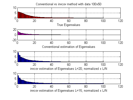
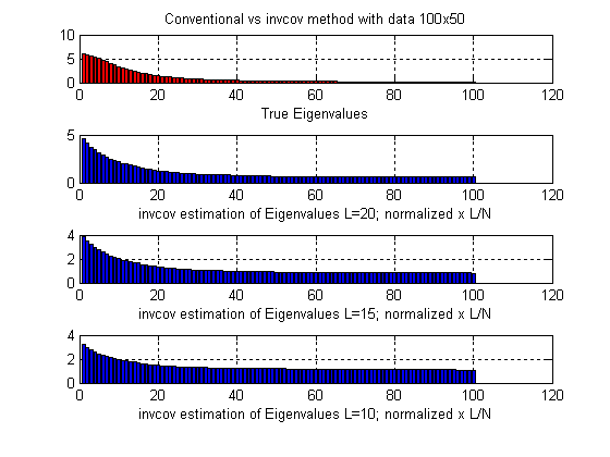
Refer to caption
Figure 1: Comparison of the eigenvalues of the true covariance matrix and sample covariance matrix vs. invcovinvcov\mathrm{invcov} estimate. The conventional eigenvalue estimate gives 50 eigenvalues that are precisely zero, which is not correct. Our invcovinvcov\mathrm{invcov} estimate is much closer to the actual eigenvalue distribution.
Refer to caption
Figure 2: Comparison of the eigenvalues of the true covariance matrix and sample covariance matrix vs. invcovinvcov\mathrm{invcov} estimate
Refer to caption
Figure 3: Comparison of the eigenvalues of the true covariance matrix and sample covariance matrix vs. invcovinvcov\mathrm{invcov} estimate
Refer to caption
Figure 4: Comparison of the eigenvalues of the true covariance matrix and sample covariance matrix vs. invcovinvcov\mathrm{invcov} estimate

Let A𝐴A be an N×N𝑁𝑁N\times N matrix we define the Frobenius norm as A2=1N2Tr(AA)subscriptnorm𝐴21superscript𝑁2Trsuperscript𝐴𝐴\|A\|_{2}=\frac{1}{N^{2}}\mathrm{Tr}(A^{*}A). In Figure 5, 6 and 7 we compare the performance of our estimator with the more standard estimator of Ledoit and Wolf [7]. The experiment was performed with a 60×60606060\times 60 true covariance matrix ΣΣ\Sigma with Toeplitz entries Σi,j=exp(1β|ij|)subscriptΣ𝑖𝑗1𝛽𝑖𝑗\Sigma_{i,j}=\exp(-\frac{1}{\beta}|i-j|) and N=30𝑁30N=30. We compute the Frobenius norm ΣinvcovL(Kx)12subscriptnormΣsubscriptinvcov𝐿superscriptsubscript𝐾𝑥12\|\Sigma-\mathrm{invcov}_{L}(K_{x})^{-1}\|_{2} for the different values of L𝐿L and we compare it with ΣKLW2subscriptnormΣsubscript𝐾𝐿𝑊2\|\Sigma-K_{LW}\|_{2}. We use β=10,50𝛽1050\beta=10,50 and 100100100. We can see that our method outperform Ledoit and Wolf for a big range of the parameter L𝐿L. We also note that in the three cases L=20𝐿20L=20 is the optimum.

Refer to caption
Figure 5: Performance comparison with respect to Ledoit and Wolf for β=10𝛽10\beta=10. The horizontal blue line is the performance of the LW estimate, our invcovinvcov\mathrm{invcov} estimate outperforms LW for L𝐿L between 15 and 22.
Refer to caption
Figure 6: Performance comparison with respect to Ledoit and Wolf for β=50𝛽50\beta=50
Refer to caption
Figure 7: Performance comparison with respect to Ledoit and Wolf for β=100𝛽100\beta=100

X Comments

Our investigation indicates that the new method presented in this article is interesting and promising from the mathematical point of view, as well as the practical one. Even though we were able to find the asymptotics formulas as well as close form expressions for invcovLsubscriptinvcov𝐿\mathrm{invcov}_{L}, and more generally for fcovLsubscriptfcov𝐿\mathrm{fcov}_{L}, both estimates for Σ1superscriptΣ1\Sigma^{-1} and f(Σ)𝑓Σf(\Sigma), there is a natural question still unanswered. How to find the optimum L𝐿L? For instance assume we know that the matrix ΣΣ\Sigma is an M×M𝑀𝑀M\times M Toeplitz distributed with entries Σi,j=exp(1β|ij|)subscriptΣ𝑖𝑗1𝛽𝑖𝑗\Sigma_{i,j}=\exp(-\frac{1}{\beta}|i-j|) with unknown β𝛽\beta. How does the optimum L𝐿L depends on M𝑀M and N𝑁N? In the simulations presented in Section IX we see that for M=60𝑀60M=60, N=30𝑁30N=30 the optimum L𝐿L is equal to 20 and it seems to be independent on the value of β𝛽\beta. We believe that this a question interesting to explore.

XI Acknowledgments

We would like to thank Thomas Bengtsson and Yuliy Baryshnikov for many helpful discussions and comments.

Appendix A Average over the permutation matrices

In this Appendix we study what happen if we substitute the average over the isotropically random unitary matrices by the set of permutation matrices. Let D𝐷D be an N×N𝑁𝑁N\times N diagonal matrix with D=diag(d1,,dN)𝐷diagsubscript𝑑1subscript𝑑𝑁D=\mathrm{diag}(d_{1},\ldots,d_{N}) and LN𝐿𝑁L\leq N. We will denote epsubscript𝑒𝑝e_{p} the orthonormal vector 1×N1𝑁1\times N in Nsuperscript𝑁\mathbb{C}^{N} whose entries are zero except at the pthsuperscript𝑝𝑡p^{\,th}–coordinate that is 1. A permutation matrix is a L×N𝐿𝑁L\times N matrix of the form

Φ=(ep1ep2epL)wherepipjforij.formulae-sequenceΦmatrixsubscript𝑒subscript𝑝1subscript𝑒subscript𝑝2subscript𝑒subscript𝑝𝐿whereformulae-sequencesubscript𝑝𝑖subscript𝑝𝑗for𝑖𝑗\Phi=\begin{pmatrix}e_{p_{1}}\\ e_{p_{2}}\\ \vdots\\ e_{p_{L}}\\ \end{pmatrix}\hskip 19.91684pt\text{where}\hskip 11.38092ptp_{i}\neq p_{j}\hskip 11.38092pt\text{for}\hskip 11.38092pti\neq j.
Theorem 2

Let D𝐷D be a diagonal matrix as before. Then

𝔼[Φ(ΦDΦ)1Φ:ΦL×Npermutation]=LND1.\mathbb{E}\,\Big{[}\Phi^{*}(\Phi D\Phi^{*})^{-1}\Phi\,\,:\,\,\Phi\,\,\,\,L\times N\,\,\mathrm{permutation}\Big{]}=\frac{L}{N}\,D^{-1}.
Proof:

We will first show that

ΦDΦ=diag(dp1,dp2,,dpL).Φ𝐷superscriptΦdiagsubscript𝑑subscript𝑝1subscript𝑑subscript𝑝2subscript𝑑subscript𝑝𝐿\Phi D\Phi^{*}=\mathrm{diag}(\,d_{p_{1}},d_{p_{2}},\ldots,d_{p_{L}}).

Given 1pN1𝑝𝑁1\leq p\leq N then epD=dpepsubscript𝑒𝑝𝐷subscript𝑑𝑝subscript𝑒𝑝e_{p}\cdot D=d_{p}\,e_{p}. Therefore,

ΦDΦΦ𝐷superscriptΦ\displaystyle\Phi D\Phi^{*} =\displaystyle= (dp1ep1dp2ep2dpLepL)(ep1Tep2TepLT)subscript𝑑subscript𝑝1subscript𝑒subscript𝑝1subscript𝑑subscript𝑝2subscript𝑒subscript𝑝2subscript𝑑subscript𝑝𝐿subscript𝑒subscript𝑝𝐿superscriptsubscript𝑒subscript𝑝1𝑇superscriptsubscript𝑒subscript𝑝2𝑇superscriptsubscript𝑒subscript𝑝𝐿𝑇\displaystyle\left(\begin{array}[]{c}d_{p_{1}}e_{p_{1}}\\ d_{p_{2}}e_{p_{2}}\\ \vdots\\ d_{p_{L}}e_{p_{L}}\\ \end{array}\right)\left(\begin{array}[]{cccc}e_{p_{1}}^{T}&e_{p_{2}}^{T}&\ldots&e_{p_{L}}^{T}\\ \end{array}\right)
=\displaystyle= diag(dp1,dp2,,dpL).diagsubscript𝑑subscript𝑝1subscript𝑑subscript𝑝2subscript𝑑subscript𝑝𝐿\displaystyle\mathrm{diag}(\,d_{p_{1}},d_{p_{2}},\ldots,d_{p_{L}}).

Hence,

(ΦDΦ)1=diag(dp11,dp21,,dpL1).superscriptΦ𝐷superscriptΦ1diagsuperscriptsubscript𝑑subscript𝑝11superscriptsubscript𝑑subscript𝑝21superscriptsubscript𝑑subscript𝑝𝐿1(\Phi D\Phi^{*})^{-1}=\mathrm{diag}(\,d_{p_{1}}^{-1},d_{p_{2}}^{-1},\ldots,d_{p_{L}}^{-1}).

Thus,

Φ(ΦDΦ)1Φ=i=1Ldpi1epiTepi.superscriptΦsuperscriptΦ𝐷superscriptΦ1Φsuperscriptsubscript𝑖1𝐿superscriptsubscript𝑑subscript𝑝𝑖1superscriptsubscript𝑒subscript𝑝𝑖𝑇subscript𝑒subscript𝑝𝑖\Phi^{*}(\Phi D\Phi^{*})^{-1}\Phi=\sum_{i=1}^{L}{d_{p_{i}}^{-1}e_{p_{i}}^{T}e_{p_{i}}}. (90)

Note that Ep:=epTepassignsubscript𝐸𝑝superscriptsubscript𝑒𝑝𝑇subscript𝑒𝑝E_{p}:=e_{p}^{T}e_{p} is the matrix that has all entries zero except at the (p,p)𝑝𝑝(p,p) entry which is 1. The total number of different permutation matrices is N!(NL)!𝑁𝑁𝐿\frac{N!}{(N-L)!}. Therefore,

𝔼[Φ(ΦDΦ)1Φ]=(NL)!N!(p1,,pL)[i=1Ldpi1Epi]𝔼delimited-[]superscriptΦsuperscriptΦ𝐷superscriptΦ1Φ𝑁𝐿𝑁subscriptsubscript𝑝1subscript𝑝𝐿delimited-[]superscriptsubscript𝑖1𝐿superscriptsubscript𝑑subscript𝑝𝑖1subscript𝐸subscript𝑝𝑖\mathbb{E}\,[\Phi^{*}(\Phi D\Phi^{*})^{-1}\Phi]=\frac{(N-L)!}{N!}\cdot\sum_{(p_{1},\ldots,p_{L})}{\Bigg{[}\sum_{i=1}^{L}{d_{p_{i}}^{-1}E_{p_{i}}}\Bigg{]}}

where the first sum is running over all the possible permutation matrices. The number of permutation matrices that have epsubscript𝑒𝑝e_{p} as one of their rows is (N1)!L!(L1)!(NL)!𝑁1𝐿𝐿1𝑁𝐿\frac{(N-1)!L!}{(L-1)!(N-L)!}. Hence,

𝔼[Φ(ΦDΦ)1Φ]𝔼delimited-[]superscriptΦsuperscriptΦ𝐷superscriptΦ1Φ\displaystyle\mathbb{E}[\Phi^{*}(\Phi D\Phi^{*})^{-1}\Phi] =\displaystyle= (NL)!N!(N1)!L!(L1)!(NL)!D1𝑁𝐿𝑁𝑁1𝐿𝐿1𝑁𝐿superscript𝐷1\displaystyle\frac{(N-L)!}{N!}\frac{(N-1)!L!}{(L-1)!(N-L)!}\cdot D^{-1}
=\displaystyle= LND1.𝐿𝑁superscript𝐷1\displaystyle\frac{L}{N}\,D^{-1}.

References

  • [1] T. L. Marzetta, A new interpretation for Capon’s maximum likelihood method of frequency-wavenumber spectrum estimation, IEEE Trans. on Acoustics, Speech, and Signal Processing, ASSP-31 (2), p. 445-449, 1983.
  • [2] T. L. Marzetta, S. H. Simon, and H. Ren, Capon-MVDR spectral estimation from singular data covariance matrix, with no diagonal loading, Proc. Fourteenth Annual Workshop on Adaptive Sensor Array Processing (ASAP 2006), M.I.T. Lincoln Laboratory, June 6-7, 2006.
  • [3] Y. V. Fyodorov and B. A. Khoruzhenko, A few remarks on Color–Flavor Transformations, truncation of random unitary matrices, Berezin reproducing kernels and Selberg type integrals, arXiv : math-ph/0610045v2, 2006.
  • [4] I. G. Macdonald, Symmetric functions and Hall Polynomials, Clarendon Press, Oxford University Press, New York, 1995.
  • [5] R. J. Muirhead, Aspects of Multivariate Statistical Theory, John Wiley & Sons, New York, 1982.
  • [6] S. Verdu and A. M. Tulino, Random Matrix Theory and Wireless Communications, Now Publishers Inc., 2004.
  • [7] O. Ledoit and M. Wolf, Some Hypothesis Tests for the Covariance Matrix when the Dimension is Large Compared to the Sample Size, Annals of Statistics, vol. 30, no. 4, pp. 1081–1102, 2002.
  • [8] J. Capon, High–Resolution Frequency Wavenumber Spectrum Analysis, Proc. IEEE, Vol. 57, 1408-1418, 1969.
  • [9] N. R. Rao and A. Edelman, The Probability Distribution of the MVDR Beamformer Outputs under Diagonal Loading, Proc. Thirteen Annual Adaptative Sensor Array Proc. Workshop, 7-8 June, 2005.
  • [10] C. D. Richmond, R. R. Nadakuditi and A. Edelman, Asymptotic Mean Square Error Performance of Diagonally Loaded Capon-MVDR Processor, Proc. Asilomar Conf. on Signals, Systems, and Computers, Pacific Grove, CA, Oct. 29-Nov. 1, 2005.
  • [11] T. L. Marzetta and B. M. Hochwald, Capacity of a Mobile Multiple-Antenna Communication Link in Rayleigh Flat Fading, IEEE Trans. Inform. Theory, vol. 45, p. 139-157, Jan. 1999.
  • [12] N. R. Draper and H. Smith, Applied regression analysis, Wiley, 1998.
  • [13] W. B. Johnson and J. Lindenstrauss, Extensions of Lipschtiz mappings into a Hilbert space, Contemp. Math., 26, p. 189-206, 1984.
  • [14] E. J. Candes and M. B. Wakin, An introduction to compressive sampling, IEEE Signal Processing Magazine, [24], March 2008.
  • [15] R. O. Duda and P. E. Hart, Pattern Classification and Scene Analysis, Wiley, 1973.
  • [16] P. Domingos and M. Pazzani, Beyond independence: conditions for the optimality of the simple Bayesian classifier, Proceedings of the Thirteenth International Conference on Machine Learning, p. 105-112, Bari, Italy, 1996.
  • [17] P. Stoica and R. Moses, Spectral Analysis of Signals, Pearson Prentice Hall, 2005.
  • [18] A. Nica and R. Speicher, Lectures on the Combinatorics of Free Probability, Cambridge University Press, 2006.
  • [19] B. Collins, J.A. Mingo, P. Sniady and R. Speicher, Second Order Freeness and Fluctuations of Random Matrices: III Higer Order Freeness and Free Cumulants, Documenta Math., vol. 12, pp. 1–70, 2007.
  • [20] D. Voiculescu, Free Probability Theory, Fields Institute Communications, 1997 .
  • [21] D. Voiculescu, K. Dykema and A. Nica, Free Random Variables, CRM Monograph Series, vol. 1, AMS, 1992.