Offsprings of a Point Vortex

Abstract

The distribution engendered by successive splitting of one point vortex are considered. The process of splitting a vortex in three using a reverse three-point vortex collapse course is analysed in great details and shown to be dissipative. A simple process of successive splitting is then defined and the resulting vorticity distribution and vortex populations are analysed.

1 Introduction

Turbulent flows are often characterized by cascade dynamics that explain the transfer of quantities (energy, enstrophy) between scales frisch . In particular, in two-dimensional turbulent flows, a striking features is the presence of an inverse energy cascade, which leads to the emergence of coherent vortices, dominating the flow dynamics Benzi86 ; Benzi88 ; McWilliams84 ; Weiss92 ; Carnevale91 , together with the direct cascade of enstrophy. In order to tackle these problems, point vortices have been commonly used with some success: indeed they can approximate the inviscid dynamics of finite-sized vortices Zabusky82 ; Vobseek97 ; Fuentes96 , as for instance in punctuated Hamiltonian models Carnevale91 ; Benzi92 . In these models, the advection of well-separated vortices is approximated via Hamiltonian point-vortex dynamics (thus inviscid i.e. dissipationless); to account for the change in the vortex population toward smaller number of bigger vortices, dissipative merging processes are then included for vortices which have approached each other closer than a certain critical distance. In decaying two-dimensional turbulence, the merging process results in fact from the interaction of a few number of close vortices Dritschel96 so that the understanding of low dimensional vortex dynamics is an essential ingredient of the whole picture Aref99 . More generally, it has been shown that point vortices can exhibit both the features of extremely high-dimensional as well as low-dimensional systems Weiss98 .

Since the pioneering work of Onsager on two dimensional turbulence Onsager49 , a statistical approach to turbulence using point vortices has also been developed. These vortex systems display negative temperature, corresponding to states where same-sign vortices bound to form larger vortices Joyce73 ; Onsager49 , although special care in the definition of the thermodynamic limit has to be donefrohlich82 . In the same spirit, stationary flows resulting from point vortices can be obtained Caglioti92 ; Robert92 ; Spineanu05 and different kinetic theories can also be derived (see for instance Chavanis07 and references therein).

Regarding the dynamical aspect, the relevance of point vortices, seen as exact solutions of the Euler equation, is still debated: indeed finite time singularities are present in the coupled dynamics of many point vortices. These singularities correspond to the collapse of three vortices Synge49 ; Novikov79 ; LKZ2000 , and can been seen as the consequences of an ill posed problem. Such singularity arises in fact naturally in the Hamiltonian point vortices dynamics. Regardless the influence of the viscosity that would become dominant at short time before the singularity, it is important to notice that the dynamics toward the three vortices collapses is in fact reversible. Thus, it is tempting to consider the reverse dynamics which would consist of vortices separation that has to be present in this Hamiltonian system! Such dynamics has been omitted until now since the number of point vortices was taken constant or only decreasing.

Therefore, in this paper we take a different perspective on the existence of this finite time singularity, using it as a potential source of vorticity and vortices. One of the perspective is to offer the possibility of a statistical mechanics approach with a varying number of vortices. At this stage, we remain within the Hamiltonian framework of point vortices and in particular we do not consider the regularization due to the viscosity for real fluid. In addition, we focus here on the statistical distribution of vorticity rather than on the coupled dynamics of the system of vortices issued of this splitting. To be more precise, in this paper our main goal is to describe the statistical properties emerging from this genuine process of vortex splitting: we consider the distributions of vortices and vortex strength resulting from this simple mechanism of successive splitting according to the reverse collapse of one point vortex. We shall refer to this result as the offsprings of a point vortex.

The paper is organized as follows, first we recall briefly the notion of point vortices, and how they naturally appear as a solution of Euler equation. We then consider the process of splitting one vortex in three. We introduce the relevant parameters and analyse briefly the preliminary consequences. In particular, we observe that this splitting is inherently a dissipative process. Finally we define simple rules for successive splitting. Computing the offsprings of a point vortex with these rules we deduce general properties for the vortices distribution in the limit of high splitting processes.

2 Basic equations

Point vortices are singular solutions of some bidimensional physical systems described by a conservation equation of what we shall call a generalised vorticity $\Omega$ given by

$$\frac{\partial\Omega}{\partial t}+\{\Omega,\psi\}=0\>,$$ (1)

where $\{\cdot,\cdot\}$ denotes the usual Poisson bracket, and $\psi$ is a stream function. The actual relation $\Omega=F(\psi)$ may depend on the considered physical system. For instance for the Euler equation it is simply given by $\Omega=-\nabla^{2}\psi$. When $\Omega=-\nabla^{2}\psi+\psi/\rho_{s}^{2}$ where $\psi$ is, in this context, related to the electric potential (in suitable units) in a plasma, $\rho_{s}$ is the hybrid Larmor radius. Point vortices are defined by a vorticity distribution given by a superposition of Dirac functions,

$$\Omega(\mathbf{r},t)=\frac{1}{2\pi}\sum_{i=1}^{N}k_{i}\delta\left(\mathbf{r}-\mathbf{r}_{i}(t)\right)\>,$$ (2)

where $\mathbf{r}=(x,y)$ is a vector in the plane of the flow, $k_{i}$ is the strength of vortex $i$ (circulation), $N$ is the total number of vortices, and $\mathbf{r}_{i}(t)$ is the vortex position at time $t$. Using this expression of the vorticity and solving the Poisson equation, in the Euler case, or the Helmholtz equation in the more general case, one obtains the current function associated to the point vortices. Thanks to the Helmholtz theorem, the motion of the vortices is determined by the value of the velocity field created by the other vortices at the position of the vortex. The point vortex motion is Hamiltonian and given by

$$k_{i}\dot{y_{i}}=-\frac{\partial H}{\partial x_{i}}:,\hskip 28.45274pt\dot{x}_{i}=\frac{\partial H}{\partial(k_{i}y_{i})}:,(i=1,\cdots,N)$$ (3)

where the Hamiltonian $H$ is given by

$$H=\frac{1}{2\pi}\sum_{i>j}k_{i}k_{j}U(|\mathbf{r}_{i}-\mathbf{r}_{j}|)$$ (4)

with for an unbounded plane $U(x)=-\log(x)$ in the Euler case, and $U(x)=\mathrm{K}_{0}(x)$ in the more general case of the plasma model (when $\rho_{s}\rightarrow\infty$ the modified Bessel function $\mathrm{K}_{0}$ tends to the logarithm). The Hamiltonian (4) exhibits clearly that a system of point vortices is invariant by translation and rotation, which implies both the conservation of the centre of vorticity and the total angular momentum, the motion of three vortices is integrable, while for four or more vortices Hamiltonian chaos come into play. When the distance between the vortices is smaller than the typical interaction length ($\rho_{s}$) the behaviour of the two systems is similar, while in the large distance limit, the $\mathrm{K}_{0}$ interaction decreases exponentially and the vortices are almost free. In the following, analytical computations will be made using the logarithmic interaction, which corresponds to the Euler flow, and we can expect the results to be qualitatively valid for the Bessel interaction as long as the vortices are not “too far” from each other.

Regarding the Hamiltonian (4), we remind that it does not represent the energy of the fluid (which is infinite already with one point vortex), but rather corresponds to an energy of interaction between the vortices and is the one that is traditionnally used when making a statistical physics approach of point vortex systems. It is however important to recall there is actually an infinite “reserve” of energy in these systems. In what follows, we abusively refer to this interaction-energy, as energy.

Let us now focus on a situation with only three vortices. In this restricted situation, it is easier to tackle the motion of the vortices by studying in fact their relative motion. Namely the three vortices form a triangle, and the relative motion describes the deformation of this triangle Synge49 ; Novikov75 ; Aref79 ; Aref83 ; LKZ2000 . The invariance by translation of (4), allows us a free choice of the origin of the plane, which we choose to be the centre of vorticity (when it exists). The other constants of motion written in a frame independent form become,

$$\left\{\begin{array}[]{l}H=-\frac{1}{2\pi}\left[k_{1}k_{2}\ln R_{3}+k_{1}k_{3}\ln R_{2}+k_{3}k_{2}\ln R_{1}\right]\\ K=k_{1}k_{2}R_{3}^{2}+k_{1}k_{3}R_{2}^{2}+k_{3}k_{2}R_{1}^{2}\>,\end{array}\right.$$ (5)

where $R_{i}=|\mathbf{r}_{j}-\mathbf{r}_{k}|$, with $i~\neq j\neq k$. In fact it has been known for a long time that the motion of vortices can lead to singular solutions and finite time singularities, the most striking one occurring for a system of three vortices resulting in the collapse of the vortices in a finite time Synge49 ; Novikov79 ; LKZ2000 or by time reversal, to an infinite expansion of the triangle formed by the vortices. The collapse or infinite expansion of the three point vortices are obtained when the following conditions are satisfied

$$K=0$$ (6)

$$\sum_{i}\frac{1}{k_{i}}=0\>,$$ (7)

the harmonic mean of the vortex strengths (7) and the total angular momentum in its frame free form (6), are both equal to zero Aref79 ; Aref83 ; Tavantzis88 .

In this paper we shall use this specific singularity and consider vorticity distribution arising from successive splitting of a point vortex according to the collapse conditions. Note that other type of singularities involving more vortices are effectively possible, however for the sake of simplicity, we restrict ourselves to reverse three-vortex collapse rules. In what follows we shall refer to the successive splitting process as the point vortex offsprings.

3 Splitting of a Point Vortex

3.1 Splitting rules

In order to be consistent with the physical properties of vortex collapse, we successively divide vortices according to the collapses rules and keep the total vorticity constant. The splitting rules from one generation $n$ of a vortex $i$ of strength $k_{i,n}$ to the next generation $n+1$ read

$$\sum_{i=1}^{3}k_{i,n+1} = k_{i,n}$$ (8)

$$\sum_{i=1}^{3}\frac{1}{k_{i,n+1}} = 0\>.$$ (9)

These equations are equivalent to

$$\sum_{i=1}^{3}k_{i,n+1} = k_{i,n}$$ (10)

$$\sum_{i=1}^{3}k_{i,n+1}^{2} = k_{i,n}^{2}\;,$$ (11)

the $k_{i,n+1}$ lie on the circle at the intersection of the sphere of radius $|k_{i,n}|$ defined by Eq. (11) and the plane defined by Eq. (10). We therefore discuss the splitting in terms of the vector $\mathbf{k}_{n+1}=(k_{1,n+1},k_{2,n+1},k_{3,n+1})$. The tip of the vector lies on a circle, hence we parametrise it with an angle $\theta_{n}$ as:

$$\mathbf{k}_{n+1}=k_{n}\left(\mathbf{a}+\sqrt{\frac{2}{3}}\left(\cos\theta_{n}\>\mathbf{u}+\sin\theta_{n}\>\mathbf{v}\right)\right)\>,$$ (12)

where $\mathbf{a}=(1,1,1)/3$, and for instance $\mathbf{u}=(1,-1,0)/\sqrt{2}$ and $\mathbf{v}=\sqrt{3}\>\mathbf{a}\wedge\mathbf{u}$. In fact the choice of $\theta_{n}$ can be restricted to be picked within the segment $[0,\>2\pi/3]$, since Eq.(12) exhibits the symmetry $k_{3,n}(\theta+2/3\pi)=k_{1,n},k_{3,n}(\theta-2/3\pi)=k_{2,n}$ and thus all configurations up to a relabelling can be obtained within this interval.

3.2 Is the splitting always possible?

We imagine that we are dealing with a system with many vortices ($2n+1$ after $n$ splittings) and consider the splitting of one point vortex according to the rules (6) and (7) in this system. The total number of vortices changes, see Fig 1 for an illustration of the process.

Regarding the energy we have

$$\delta H_{n} = H_{n+1}-H_{n}=-\frac{1}{4\pi}\ln\Lambda_{n}\>,$$ (13)

$$= -\frac{1}{4\pi}\left[k_{1}k_{2}\ln R_{3}+k_{1}k_{3}\ln R_{2}+k_{3}k_{2}\ln R_{1}\>,\right]$$ (14)

where for instance the vortex $k_{N}=k_{1}+k_{2}+k_{3}$ was split in three. In order to be dynamically compatible, we first neglect the influence of the other vortices (which are considered far enough to not interfere locally), but still we need to make sure that there is at least one triangle satisfying the conditions and define the value of $\delta H_{n}$ associated with the splitting. For that purpose after the splitting we name $2$ and $3$ the vortices whose strengths have the same sign with $|k_{2}|<|k_{3}|$, exponentiating Eq. (13) gives

$$R_{3}^{k_{1}k_{2}}R_{2}^{k_{1}k_{3}}R_{1}^{k_{2}k_{3}}=\Lambda_{n}\>,$$ (15)

then we divide by one noticing that $R_{1}^{\sum k_{i}k_{j}}=1$, and obtain

$$\left(\frac{R_{3}}{R_{1}}\right)^{k_{1}k_{2}}\left(\frac{R_{2}}{R_{1}}\right)^{k_{1}k_{3}}=\Lambda_{n}\>.$$ (16)

Since the collapse is scale free (self-similar), we choose $R_{1}$ as our length units, note $r_{2}=R_{2}/R_{1}$, $r_{3}=R_{3}/R_{1}$ and arrive at

$$r_{2}=\Lambda_{n}^{1/k_{3}k_{1}}r_{3}^{-k_{2}/k_{3}}\>.$$ (17)

The condition (6) becomes once rescaled

$$k_{1}k_{2}r_{3}^{2}+k_{1}k_{3}r_{2}^{2}+k_{3}k_{2}=0\>,$$ (18)

combining this last expression with (7) we have

$$k_{2}(r_{3}^{2}-1)+k_{3}(r_{2}^{2}-1)=0\>,$$ (19)

and noting $\alpha=k_{2}/k_{3}(<1)$, we finally obtain

$$\alpha r_{3}^{2(1+\alpha)}+\Lambda_{n}^{2/k_{1}k_{3}}=(1+\alpha)r_{3}^{2\alpha}\>.$$ (20)

$\Lambda_{n}$ being positive, $\alpha X^{1+\alpha}-(1+\alpha)X^{\alpha}$ shows that $r_{3}^{2}\in]0\>;1+1/\alpha[$ and that $0<\Lambda_{n}^{2/k_{1}k_{2}}\leq 1$. The equality $\Lambda_{n}=1$ being reached for $r_{3}=1$ which implies an equilateral triangle. This last configuration has to be excluded as it is dynamically a fix point, i.e the triangle does not expand or shrink hence can not be a starting point for a vortex splitting. So , since $k_{1}k_{3}<0$, this means that $\Lambda_{n}>1$ and that $\delta H_{n}=-\frac{1}{4\pi}\ln\Lambda_{n}<0$. The splitting of a vortex in three is thus a dissipative process!

We now enforce that the solution is a triangle, using the rescaled variables this means that

$$1=r_{2}^{2}+r_{3}^{2}-2r_{3}r_{2}\cos\varphi\>,$$ (21)

which implies (using Eq. (19))

$$\cos\varphi=\frac{r_{3}^{2}(1-\alpha)+\alpha}{2r_{3}\sqrt{1+\alpha-\alpha r_{3}^{2}}}\>.$$ (22)

The right hand side of Eq. (22) is always positive, so $-\pi/2<\varphi<\pi/2$. The minimum is obtained for $r_{3}^{2}=\alpha(1+\alpha)/(1+\alpha^{2})$ and equal to $\alpha^{1/2}/(1+\alpha)$, which is always smaller than one. Therefore, there is always a range of possibilities available for $r_{3}$ and the splitting is always possible. Note that for a given value of $r_{3}$ the two mirroring shapes of the triangle are possible, one giving rise to expansion (splitting) the other one to collapse.

4 Vorticity distributions

We are now interested in the vorticity distribution we obtain from such process. For this purpose we compute

Figure 1: Simple 5th order vortex lineage. In this picture we see that after $8$ splittings, $4$ vortices are remaining on level $3$.

different trees originating from one vortex of strength $k=1$ as depicted in Fig. 1. The distributions are computed by successive vortex splitting. After each division, a vortex is chosen randomly among the global population and is split according to the reverse collapse rules, the division is the result of the uniformly random choice of an angle $\theta_{n}$ (see Eq. (12)). Other possible rules made by assigning different probabilities on vortices will be explored in future work.

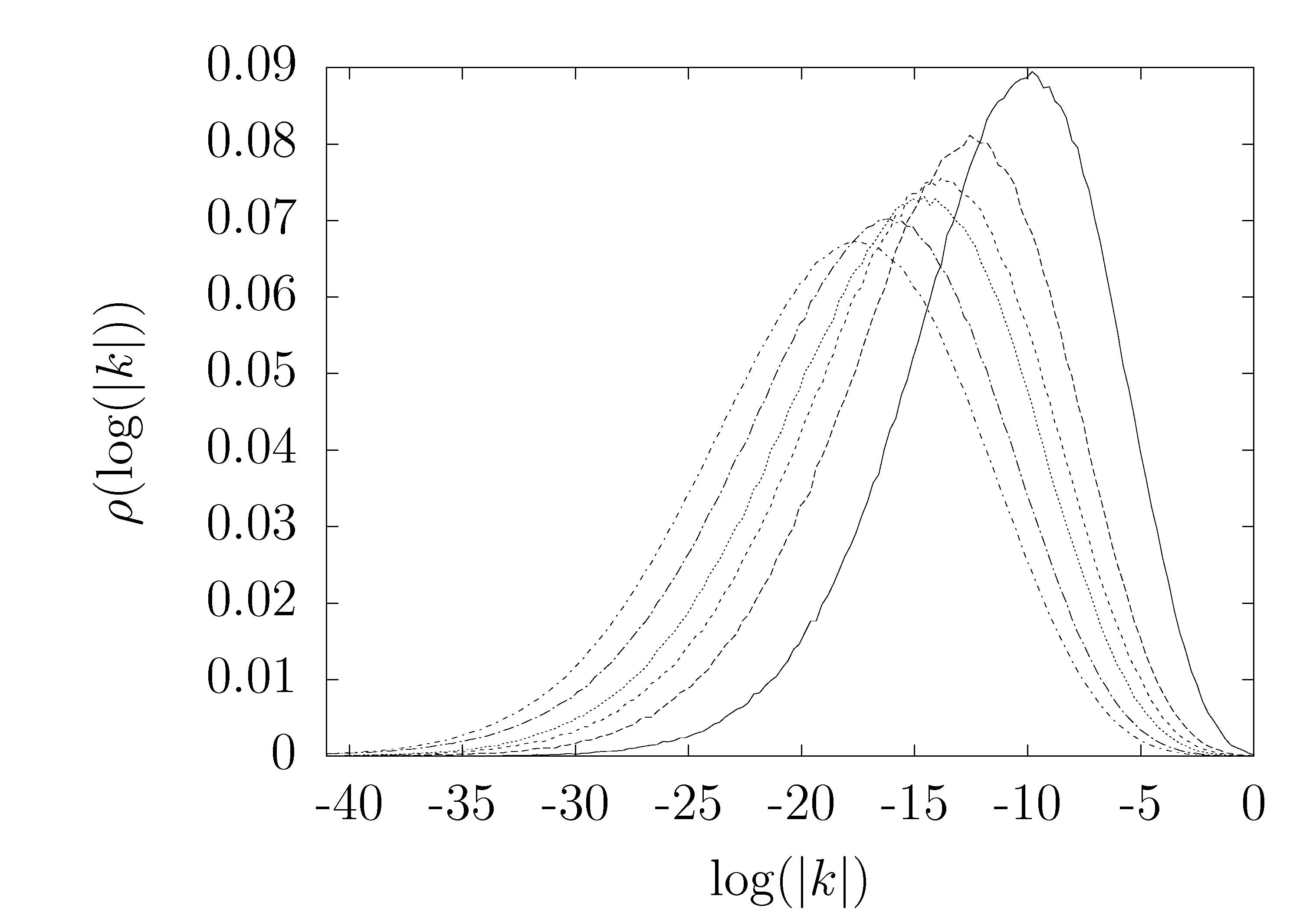
Figure 2: Probability density function (PDF) of the absolutes values of vortex strengths after respectively (from right to left) $10^{3}$, $5\>10^{3}$, $10^{4}$, $2\>10^{4}$, $5\>10^{4}$, $10^{5}$ vortex splits. The PDF have been averaged over $64$ trees, for the large values and up to $512$ trees for the smallest ones. The shape appears as self-similar.

Results of the obtained distributions are depicted in Fig. 2. We shall notice that the chosen rules gives rise to a large spectrum of vorticities (see the logarithmic scale in Fig.2). We notice as well that as the number of division increases the distribution spreads and the location of its maximum is slowly moving towards smaller values of the vorticity, moreover, the evolution of the distribution appears to have some kind of self-similar behaviour.

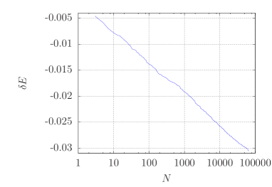
Figure 3: Variation of energy versus number of created vortices. The curve has been averaged over $100$ trees. Splittings have been performed up to $N=65537$ vortices starting from one vortex of strength $k_{0}=1$. One can notice a small logarithmic decay of energy versus the number of vortices, of the type $\delta E\approx-\lambda\log_{10}(N)$ with $\lambda\approx 5.9\>10^{-3}$.

In the same spirit the variation of energy as a function of generated vortices can be monitored. Results are shown in Fig. 3 and show a slow logarithmic decay of the total energy.

In order to analyse this in more details we need to characterise the lineage (see Fig. 1) after a given number of splittings. We will note the total number of splittings that occurred $n$. These successive divisions generate a tree (the phase space of the process) with $3^{n}$ leaves at the extremities. Each division results in the choice of an angle $\theta_{i}$. Now let us consider a particular “lineage” of order $n$, it gives rise to a family of $N=2n+1$ vortices. At each step of the division process (from $n$ to $n+1$) we choose any already existing vortex and split it with the rules (12). The trajectory in phase space corresponds to a connected graph with $2n+1$ leaves starting from the top of the tree and of total length $3n+1$. The number of possible graphs on the tree after $n$ splittings is: $(2n+1)!/(2^{n}n!)$. To move further on, and due to the large amount of possible graphs, we consider the global occupation $M_{i}$ of the level $i$ (see Fig. 1). We note $M_{i}(n)$ the average number of leaves at level $i$ at time $n$.

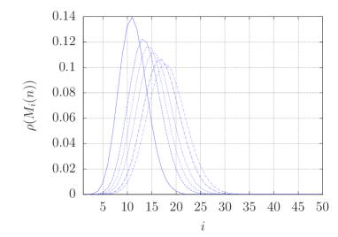
Figure 4: Probability density function (PDF) of the occupation of each generation $M$ after respectively (from left to right) $10^{3}$, $5\>10^{3}$, $10^{4}$, $2\>10^{4}$, $5\>10^{4}$, $10^{5}$ vortex splits. The PDF have been computed using the mean field equations (23). The shape appears as self-similar and is reminiscent of what is observed in Fig. 2.

Then we have

$$M_{i}(n+1)=M_{i}(n)+3\frac{M_{i-1}(n)}{2n+1}-\frac{M_{i}(n)}{2n+1}\>,$$ (23)

with initial conditions $M_{0}(0)=1$, $M_{n>0}(0)=0$. It is easy to integrate numerically this equation in order to have an idea of the solution. We find that the form

$$M_{i}(n)=a_{i}\frac{\left(\log(2n+1)\right)^{i-1}}{\sqrt{2n+1}}$$ (24)

is solution, with $a_{i}=3a_{i-1}/(2(i-1))$, i.e.

$$a_{i}=\left(\frac{3}{2}\right)^{i-1}\frac{a_{1}}{(i-1)!}\>.$$ (25)

This can be checked easily by induction, we assume that $M_{i-1}$ is of this form, and then we can solve Eq. (23) for $M_{i}$ in the continuous time limit in which it becomes

$$\frac{dM_{i}}{dn}=3\frac{M_{i-1}}{2n+1}-\frac{M_{i}}{2n+1}\>.$$ (26)

In this way we obtain that at a fixed level $i$, the occupancy $M_{i}$ first increases with time, then decreases, with a maximum at $n^{*}(i)\sim\exp(2i)$. At fixed time $n$ on the other hand, $M_{i}(n)$ has a maximum at $i^{*}\sim 3\log(2n+1)/2$.

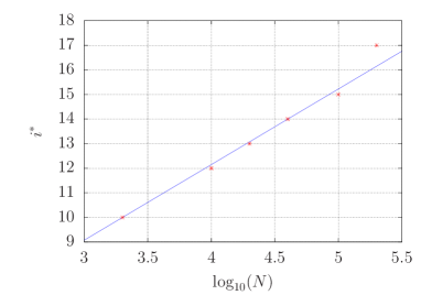
Figure 5: Maximum $i^{*}$ versus number of vortices $N$. $i^{*}$ is obtained from the distributions displayed in Fig. 4. A linear scaling is observed as expected, with a measured slope of $\sim 3.1$, “close to the expected value $3/2\times\ln 10\approx 3.45$” .

A numerical integration of the global populations given by Eq. (23) is displayed in Fig. 4. One can notice similarities with the distributions of vorticity although the distributions are more peaked. In order to test as well our analysis, the location of the maximum of the distribution is displayed in Fig. 5 and a good agreement with the logarithmic law is found.

Let us now compute the distribution of vorticity $\rho(k,n)$ assuming we know the occupancy $M_{i}(n)$. Hence let us consider a vortex living in the generation $i$. It has been the result of $i$ splitting. Since the splitting rules (12) have no preferred order (as mentioned earlier they permute if we add $2\pi/3$ to the random angle), we assume that the obtained vortex is always the third vortex hence its absolute vorticity $k$ will end up being

$$k=\frac{1}{3^{i}}\prod_{j=1}^{i}(1-2\sin\theta_{j})\>,$$ (27)

and consequently its logarithm is

$$\log|k|=\sum_{j=1}^{i}\log|1-2\sin\theta_{j}|-i\log 3\>,$$ (28)

with $\theta_{j}$ being uniformly distributed random variables in $[0\>2\pi[$. We can then gather the probability distribution of vortex strengths at generation $i$, which we note $\rho_{i}(k)$. And thus the vorticity distribution after $N$ division writes

$$\rho(k,n)=\sum_{i}\rho_{i}(k)\rho(M_{i},n)\>,$$ (29)

with $\rho(M_{i},n)=M_{i}/(2n+1)$.

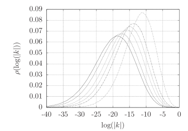
Figure 6: Probability density function (PDF) of the absolutes values of vortex strengths after respectively (from right to left) $10^{3}$, $5\>10^{3}$, $10^{4}$, $2\>10^{4}$, $5\>10^{4}$, $10^{5}$ vortex splits. The PDF have been computed using Eq.(29), where we took into account only up to generation $i=40$. The results appear to be coherent with what is displayed in Fig. 2.

In order to check these results, we compute $\rho(k,n)$ using Eq.(29) and compare the results to those displayed in Fig. 2. In fact, given the shape of the occupancy $M_{i}(n)$, we can compute $\rho(k,n)$ using only a “few” distributions $\rho_{i}(k)$. For instance in Fig. 6 we computed the $\rho_{i}(k)$ taking into account in the tree the vortices only up to generation $i=40$. We notice as well a very similar behaviour as the one displayed in Fig. 2.

5 Conclusion

This paper is a first attempt at analysing the distribution of vorticities originating from one point vortex using a dynamically compatible process, namely a reverse collapse route with the conservation of total vorticity. The splitting process has been analysed in great details and shown to be dissipative. Afterwards a simple process consisting of randomly successive splittings is proposed and the resulting distributions have been analysed. Analytical computation of the proposed process have been made, resulting for instance in the computation of the vorticity distribution after $n$ consecutive splitting of vortices and show very good agreement with the numerical simulation of the process. This paper is a first step for further work. One could for instance modify the splitting rules in order to obtain a conservative process, but also could try to pick vortices and change how the splitting is done, with a non uniform probabilities, such as a Gibbsian one and analyse the resulting distributions. In other words, we could perform statistical physics of point vortices allowing a varying number of vortices according to the collapse rules, and see if this possibility changes the equilibrium features. Last but not least, it will be important to compare the obtained distribution with real data involving physical stochastic processes. In particular, it is tempting to compare the vortex distribution obtained with this proposed mechanism or its variants with experimental results obtained on two-dimensional physical flows. Remarkably, one has to notice that, starting with a positive vortex, the reverse collapse course induces naturally the creation of negative vortices, thus the engendered distributions will consist of both positive and negative vortices. Work is currently under way to analyse these different possibilities.

- (1) U. Frisch "Turbulence: the legacy of A.N. Kolmogorov", Cambridge Univ. Press (1995).
- (2) R. Benzi, G. Paladin, S. Patarnello, P. Santangelo, A. Vulpiani, J. Phys. A 19, 3771 (1986)
- (3) R. Benzi, S. Patarnello, P. Santangelo, J. Phys. A 21, 1221 (1988)
- (4) J.C. McWilliams, J. Fluid Mech. 146, 21 (1984)
- (5) J.B. Weiss, J.C. McWilliams, Phys. Fluids A 5, 608 (1992)
- (6) C.F. Carnevale, J.C. McWilliams, Y. Pomeau, J.B. Weiss, W.R. Young, Phys. Rev. Lett. 66, 2735 (1991)
- (7) N.J. Zabusky, J.C. McWilliams, Phys. Fluids 25, 2175 (1982)
- (8) P.W.C. Vobseek, J.H.G.M. van Geffen, V.V. Meleshko, G.J.F. van Heijst, Phys. Fluids 9, 3315 (1997)
- (9) O.U. Velasco Fuentes, G.J.F. van Heijst, N.P.M. van Lipzig, J. Fluid Mech. 307, 11 (1996)
- (10) R. Benzi, M. Colella, M. Briscolini, P. Santangelo, Phys. Fluids A 4, 1036 (1992)
- (11) J.B. Weiss, A. Provenzale, J.C. McWilliams, Phys. Fluids 10, 1929 (1998)
- (12) D.G. Dritschel, N.J. Zabusky, Phys. Fluids 8, 1252 (1996)
- (13) H. Aref, Turbulent Statistical dynamics of a system of point vortice (Birkhäuser Verlag, 1999), p. 151, Trends in Mathematics, ISBN 978-3-7643-6150-1
- (14) L. Onsager, Nuovo Cimento, Suppl. 6, 279 (1949)
- (15) G. Joyce, D. Montgomery, J. Plasma Phys. 10, 107 (1973)
- (16) J. Fröhlich, D. Ruelle, Commun. Math. Phys. 87, 1 (1982)
- (17) E. Caglioti, P.L. Lions, C. Marchioro, M. Pulvirenti, Commun. Math. Phys. 143, 501 (1992)
- (18) R. Robert, J. Sommeria, Phys. Rev. Lett. 69(19), 2776 (1992)
- (19) F. Spineanu, M. Vlad, Phys. Rev. Lett. 95(23), 235003 (2005)
- (20) P.H. Chavanis, M. Lemou, Eur. Phys. J. B 59, 217 (2007)
- (21) J.L. Synge, Can. J. Math. 1, 257 (1949)
- (22) E.A. Novikov, Y.B. Sedov, Sov. Phys. JETP 22, 297 (1979)
- (23) X. Leoncini, L. Kuznetsov, G.M. Zaslavsky, Phys. Fluids 12, 1911 (2000)
- (24) E.A. Novikov, Sov. Phys. JETP 41, 937 (1975)
- (25) H. Aref, Phys. Fluids 22, 393 (1979)
- (26) H. Aref, Ann. Rev. Fluid Mech. 15, 345 (1983)
- (27) J. Tavantzis, L. Ting, Phys. Fluids 31, 1392 (1988)