Asymptotics and optimal bandwidth selection for highest density region estimation

Abstract

We study kernel estimation of highest-density regions (HDR). Our main contributions are two-fold. First, we derive a uniform-in-bandwidth asymptotic approximation to a risk that is appropriate for HDR estimation. This approximation is then used to derive a bandwidth selection rule for HDR estimation possessing attractive asymptotic properties. We also present the results of numerical studies that illustrate the benefits of our theory and methodology.

T1Supported in part by Australian Research Council Grant DP055651.

and

1 Introduction

A highest-density region (HDR) for a measurement of interest is a region where the underlying density function exceeds some nominal threshold. Given a random sample from that density, HDR estimation typically involves determination of regions where an estimated density is high. Kernel density estimation is the most common approach, but its performance is heavily dependent on the choice of the bandwidth parameter. Automatic selection of a good bandwidth for HDR estimation is the overarching goal of this article.

Figure 1 illustrates the bandwidth selection issue for HDR estimation. The left panel shows five kernel density estimates based on random samples of size 1000 from the normal mixture $\frac{2}{3}N(0,1)+\frac{1}{3}N(0,\frac{1}{100})$ density [Density 4 of Marron and Wand (1992)]. In each case the bandwidth is chosen to minimize the integrated squared error (ISE). In the right panel the same random samples are used, but, instead, the bandwidths are chosen to minimize an error appropriate for estimation of the 20% HDR (defined formally in Section 2). This region is shown as a thick horizontal line at the base of the plot. It is clear from Figure 1 that optimality for HDR estimation is quite different from ISE-optimality. Low ISE requires that the two curves be close to each other over the whole real line. However, good estimation of the 20% HDR only requires that the 20% HDRs of the kernel density estimates are close to the true region. In particular, the sharp mode of the underlying density has no bearing upon the HDR and there is no need to estimate it well. For this density it is apparent that a bandwidth considerably larger than ISE-optimal bandwidth is best for estimation of the 20% HDR.

Figure 1: Left panel: five kernel density estimates based on random samples of size 1000 simulated from the density depicted by the dashed curve. Each estimate is based on the optimal bandwidth with respect to integrated squared error. Right panel: same as the left panel except that the bandwidth is chosen to minimize the error for estimation of the 20% highest-density region. This region is shown as a thick horizontal line at the base of the plot and its boundaries are shown as dashed vertical lines.

In this article we study an asymptotic risk associated with kernel-based HDR estimation and use our theory to develop a plug-in type bandwidth selector. Attractive asymptotic properties of our bandwidth selector are established and good performance is illustrated on simulated data. A self-contained function for use in the R environment [R Development Core Team (2008)] is made available on the Internet.

The HDR estimation problem has an established literature. Contributions include Hartigan (1987), Müller and Sawitzki (1991), Polonik (1995), Hyndman (1996), Tsybakov (1997), Baíllo, Cuesta-Albertos and Cuevas (2001), Baíllo (2003), Cadre (2006), Jang (2006), Rigollet and Vert (2009) and Mason and Polonik (2009). Mason and Polonik (2009) provide a thorough literature review for the problem. Alternative terminology includes estimation of the density contours, density level sets and excess mass regions. This literature is, however, mainly concerned with theoretical results unconnected with the bandwidth selection problem. Jang (2006) is an applied paper on the use of HDR estimation for astronomical sky surveys. However, the bandwidths used there are chosen via classical ISE-based plug-in strategies. The present paper is, to our knowledge, the first to derive theory and bandwidth selection rules that are specifically tailored to the HDR estimation problem.

While our proposed practical bandwidth selector relies on asymptotic approximations, its development comes at a time when sample sizes in applications that benefit from smoothing techniques are becoming very large. The area of application that led to this research, flow cytometry, typically has sample sizes in the hundreds of thousands. The astronomical application in Jang (2006) involves sample sizes in the tens of thousands. Another HDR application is approximation of the highest posterior density region of a parameter in a Bayesian analysis, where only a sample from that density is available. In this situation, the sample, most typically obtained using Markov chain Monte Carlo methods, can arbitrarily large in size.

Section 2 presents an approximation to the HDR asymptotic risk. Numerical studies support its use for bandwidth selection. In Section 3 we describe plug-in strategies for bandwidth selection. Asymptotic performance results are established and a simulation study demonstrates practical efficacy. We conclude with an example on daily temperature maxima in Melbourne, Australia. Proofs are deferred to an Appendix.

2 Asymptotic risk results

Let $f$ be a probability density function on the real line. For $\tau\in(0,1)$, define

$$f_{\tau}=f_{\tau}(f)=\inf\biggl{\{}y\in(0,\infty)\dvtx\int_{-\infty}^{\infty}f(x)\mathbh{1}_{\{f(x)\geq y\}}\,dx\leq 1-\tau\biggr{\}}.$$

We call $R_{\tau}=\{x\in\mathbb{R}\dvtx f(x)\geq f_{\tau}\}$ the $100(1-\tau)$% highest-density region of $f$ [cf. Hyndman (1996)]. If $(X_{n})$ is a sequence of independent random variables with density $f$, the kernel estimator of $f(x)$ based on $X_{1},\ldots,X_{n}$ is

$$\widehat{f}_{h}(x)=\frac{1}{nh}\sum_{i=1}^{n}K\biggl{(}\frac{x-X_{i}}{h}\biggr{)},$$

where $K\dvtx\mathbb{R}\rightarrow\mathbb{R}$ satisfies $\int K(x)\,dx=1$, and is called a kernel and $h>0$ is called the bandwidth. Let $\widehat{f}_{h,\tau}=f_{\tau}(\widehat{f}_{h})$ denote the plug-in estimator of $f_{\tau}$, so that

$$\widehat{f}_{h,\tau}=\inf\biggl{\{}y\in(0,\infty)\dvtx\int_{-\infty}^{\infty}\widehat{f}_{h}(x)\mathbh{1}_{\{\widehat{f}_{h}(x)\geq y\}}\,dx\leq 1-\tau\biggr{\}}.$$

The corresponding plug-in estimator of $R_{\tau}$ is then $\widehat{R}_{h,\tau}=\{x\in\mathbb{R}\dvtx\widehat{f}_{h}(x)\geq\widehat{f}_{h,\tau}\}$.

Given two Borel subsets $A$ and $B$ of $\mathbb{R}$, we define their proximity through a measure on their symmetric difference $A\triangle B=(A\cap B^{c})\cup(A^{c}\cap B)$. The particular measure $\mu_{f}$ we consider is given by

$$\mu_{f}(C)=\int_{C}f(x)\,dx$$

for all Borel subsets $C$ of $\mathbb{R}$. The error $\mu_{f}(\widehat{R}_{h,\tau}\triangle R_{\tau})$ is then then the probability of an observation from $f$ lying in precisely one of $\widehat{R}_{h,\tau}$ and $R_{\tau}$. Compared with Lebesgue measure, $\mu_{f}$ puts more weight on regions where the data will tend to be denser. It also has the advantage of admitting a simple Monte Carlo approximation. This is important in higher-dimensional settings where exact computation of $\mu_{f}(C)$ is difficult.

In Theorem 1, we derive a uniform-in-bandwidth asymptotic expansion for the risk $\mathbb{E}\{\mu_{f}(\widehat{R}_{h,\tau}\triangle R_{\tau})\}$, which can facilitate a theoretical, optimal choice of bandwidth (cf. Corollary 2). This in turn motivates practical bandwidth selection algorithms whose performance is studied in Theorems 3 and 4. We will make use of the following conditions on the underlying density, bandwidth sequence and kernel:

1. [(A1):]

2. $f$ is uniformly continuous on $\mathbb{R}$. There exist finitely many points $x_{1}<\cdots<x_{2r}$ such that $f(x_{j})=f_{\tau}$ for $j=1,\ldots,2r$, and moreover there exists $\delta>0$ such that $f$ is twice continuously differentiable in $\bigcup_{j=1}^{r}[x_{2j-1}-\delta,x_{2j}+\delta]$ with $f^{\prime}(x_{2j-1})>0$ and $f^{\prime}(x_{2j})<0$ for $j=1,\ldots,r$.

3. Let $h^{-}=h_{n}^{-}$ and $h^{+}=h_{n}^{+}$ be nonnegative sequences such that $h^{-}\leq h^{+}$, such that $n(h^{-})^{4}/\sqrt{\log(1/h^{-})}\rightarrow\infty$ and such that $h^{+}\rightarrow 0$ as $n\rightarrow\infty$. Then $h=h_{n}$ is a sequence with $h_{n}^{-}\leq h_{n}\leq h_{n}^{+}$ for all $n$.

4. The kernel $K$ is nonnegative, continuously differentiable, of bounded variation, and satisfies $\int xK(x)\,dx=0$ and $\mu_{2}(K)\equiv\int x^{2}K(x)\,dx<\infty$. Moreover, $K^{\prime}$ is of bounded variation, and satisfies $\int K^{\prime}(x)^{2}\,dx<\infty$.

Assumption (A1) in particular implies that $f$ has a $\gamma$-exponent with $\gamma=1$ at level $f_{\tau}$—in other words, there exists $C>0$ such that

$$\mu_{f}(\{x\in\mathbb{R}\dvtx|f(x)-f_{\tau}|\leq\varepsilon\})\leq C\varepsilon$$

for sufficiently small $\varepsilon>0$. This type of assumption is common in the literature for this problem [cf. Polonik (1995), Rigollet and Vert (2009)]. Although there are many parts to condition (A3), none is very restrictive. Under (A1), $f_{\tau}$ is the unique positive real number satisfying $\int f(x)\mathbh{1}_{\{f(x)\geq f_{\tau}\}}\,dx=1-\tau$. In fact, in the course of the proof of Theorem 1 below, we will show that under conditions (A1), (A2) and (A3), $\widehat{f}_{h,\tau}$ has an analogous property: that is, with probability one, for all $n$ sufficiently large, $\widehat{f}_{h,\tau}$ is the unique positive real number satisfying

$$\int\widehat{f}_{h}(x)\mathbh{1}_{\{\widehat{f}_{h}(x)\geq\widehat{f}_{h,\tau}\}}\,dx=1-\tau.$$

Let $\Phi$ and $\phi$ denote the standard normal distribution function and density function, respectively, and write $R(K)=\int K^{2}(x)\,dx$. Define the quantities

$$\qquad\quad D_{1} = \frac{1}{2}\mu_{2}(K)\Biggl{\{}\sum_{j=1}^{2r}\frac{1}{|f^{\prime}(x_{j})|}\Biggr{\}}^{-1}\Biggl{[}\sum_{j=1}^{2r}\frac{f^{\prime\prime}(x_{j})}{|f^{\prime}(x_{j})|}$$

$$\hskip 122.0pt{}+\frac{1}{f_{\tau}}\sum_{j=1}^{r}\{f^{\prime}(x_{2j})-f^{\prime}(x_{2j-1})\}\Biggr{]},$$

$$D_{2} = R(K)f_{\tau}\Biggl{\{}\sum_{j=1}^{2r}\frac{1}{|f^{\prime}(x_{j})|}\Biggr{\}}^{-2}\sum_{j=1}^{2r}\frac{1}{f^{\prime}(x_{j})^{2}}\quad\mbox{and}$$

$$D_{3,j} = \frac{R(K)f_{\tau}}{|f^{\prime}(x_{j})|}\Biggl{\{}\sum_{k=1}^{2r}\frac{1}{|f^{\prime}(x_{k})|}\Biggr{\}}^{-1},\qquad j=1,\ldots,2r.$$

Theorem 1

Assume (A1), (A2) and (A3). Then

$$\mathbb{E}\{\mu_{f}(\widehat{R}_{h,\tau}\triangle R_{\tau})\} = \sum_{j=1}^{2r}\biggl{[}\frac{B_{1,j}\phi(B_{2,j}n^{1/2}h^{5/2})}{(nh)^{1/2}}$$

$$\hskip 19.2pt{}+B_{3,j}h^{2}\{2\Phi(B_{2,j}n^{1/2}h^{5/2})-1\}\biggr{]}+o\biggl{(}\frac{1}{(nh)^{1/2}}+h^{2}\biggr{)}$$

as $n\rightarrow\infty$, uniformly for $h\in[h^{-},h^{+}]$, where

$$B_{1,j} = 2f_{\tau}\frac{\{R(K)f_{\tau}-2D_{3,j}+D_{2}\}^{1/2}}{|f^{\prime}(x_{j})|},$$

$$B_{2,j} = \frac{|{1/2}\mu_{2}(K)f^{\prime\prime}(x_{j})-D_{1}|}{\{R(K)f_{\tau}-2D_{3,j}+D_{2}\}^{1/2}}$$

and

$$B_{3,j}=f_{\tau}\frac{|{1/2}\mu_{2}(K)f^{\prime\prime}(x_{j})-D_{1}|}{|f^{\prime}(x_{j})|}.$$

The nature of this result is somewhat different from the results in the existing literature which have tended to focus (sometimes in more general settings) on the order in probability or almost surely of $\mu_{f}(\widehat{R}_{h,\tau}\triangle R_{\tau})$ or related measures [e.g., Baíllo, Cuesta-Albertos and Cuevas (2001), Baíllo (2003)]. More recent works have derived results on the limiting behavior of suitably scaled and/or centered versions of $\mu_{f}(\widehat{R}_{h,\tau}\triangle R_{\tau})$ [e.g., Cadre (2006), Mason and Polonik (2009)]. Rigollet and Vert (2009) provide a finite sample upper bound for the risk, uniformly over certain Hölder classes, with an unspecified constant in the bound. While these theoretical results are certainly of considerable interest, our aim in providing the asymptotic expansion in Theorem 1 is to facilitate practical bandwidth selection algorithms for this problem—see Section 3.

In the course of the proof of Theorem 1, it is shown that

$$R(K)f_{\tau}-2D_{3,j}+D_{2}=\lim_{n\rightarrow\infty}(nh)\operatorname{Var}\bigl{(}\widehat{f}_{h}(x_{j})-\widehat{f}_{h,\tau}\bigr{)}>0,$$

so that each $B_{1,j}$ is positive. Moreover $B_{2,j}$ and $B_{3,j}$ are nonnegative, and are positive for at least one $j$. Indeed, $B_{2,j}$ and $B_{3,j}$ are certainly positive whenever $f^{\prime\prime}(x_{j})\geq\sum_{k=1}^{2r}w_{k}f^{\prime\prime}(x_{k})$, where the weights $w_{k}\propto 1/|f^{\prime}(x_{k})|$ sum to 1. However, this condition on $f^{\prime\prime}(x_{j})$ is far from necessary for $B_{2,j}$ and $B_{3,j}$ to be positive.

It is easily seen from Theorem 1 that for any sequence of bandwidths satisfying (A2), if $nh^{5}$ is not bounded away from zero and infinity then $n^{2/5}\mathbb{E}\{\mu_{f}(\widehat{R}_{h,\tau}\times\triangle R_{\tau})\}\rightarrow\infty$ along a subsequence. On the other hand, if $nh^{5}$ is bounded away from zero and infinity, then $n^{2/5}\mathbb{E}\{\mu_{f}(\widehat{R}_{h,\tau}\triangle R_{\tau})\}$ is bounded. Notice that all such sequences are permitted by the condition (A2). Focusing our attention on bandwidth sequences of order $n^{-1/5}$ and substituting $x=n^{1/2}h^{5/2}$, we have

$$\lim_{n\rightarrow\infty}n^{2/5}\mathbb{E}\{\mu_{f}(\widehat{R}_{h,\tau}\triangle R_{\tau})\}=\sum_{j=1}^{2r}\biggl{[}\frac{B_{1,j}\phi(B_{2,j}x)}{x^{1/5}}+B_{3,j}x^{4/5}\{2\Phi(B_{2,j}x)-1\}\biggr{]}.$$

Writing this limit as $g(x)\equiv\sum_{j=1}^{2r}g_{j}(x)$, we see that $g$ is continuous on $(0,\infty)$ with $g(x)\rightarrow\infty$ as $x\rightarrow 0^{+}$ and as $x\rightarrow\infty$, so $g$ attains its minimum. If $j$ is such that $B_{2,j}$ and $B_{3,j}$ are positive, then it can be shown (cf. the proof of Corollary 2 below), that $g_{j}$ has a unique minimum. This unique minimizer represents the asymptotically optimal bandwidth for estimating the risk in a small neighborhood of $x_{j}$. Although we typically expect the minimum of $g$ to be unique, the complicated nature of the function $g$ and the coefficients $B_{1,j}$, $B_{2,j}$ and $B_{3,j}$ make it difficult to prove this assertion without additional conditions. The following corollary gives the desired result in one restricted case; however, we anticipate that the result in fact holds much more widely.

Corollary 2

Assume (A1) and (A3). Assume further that in (A1) we have $r=1$ and the underlying density $f$ is symmetric about some point on the real line. Then there exists a unique $c_{\mathrm{opt}}\in(0,\infty)$, depending on $f$ and $K$ but not $n$, such that any sequence of bandwidths $(h_{\mathrm{opt}})$ that minimizes $\mathbb{E}\{\mu_{f}(\widehat{R}_{h,\tau}\triangle R_{\tau})\}$ satisfies

$$h_{\mathrm{opt}}=c_{\mathrm{opt}}n^{-1/5}\{1+o(1)\}$$

as $n\rightarrow\infty$.

The additional hypotheses on $f$ imply that $B_{1,j}$, $B_{2,j}$ and $B_{3,j}$ do not depend on $j$, and in fact in the presence of (A1) and (A3), the conclusion of the corollary also holds under this (weaker) condition, as can be seen from the proof.

2.1 Numerical assessment of risk approximation

Theorem 1 yields the asymptotic risk approximation

$$\mathbb{E}\{\mu_{f}(\widehat{R}_{h,\tau}\triangle R_{\tau})\} \simeq \sum_{j=1}^{2r}\biggl{[}\frac{B_{1,j}\phi(B_{2,j}n^{1/2}h^{5/2})}{(nh)^{1/2}}$$

$$\hskip 18.8pt{}+B_{3,j}h^{2}\{2\Phi(B_{2,j}n^{1/2}h^{5/2})-1\}\biggr{]}.$$

In Section 3 we use the right-hand side of (2.1) to develop plug-in bandwidth selection strategies. However, it is prudent to first assess the quality of this approximation to the risk. We now do this through some numerical examples.

For a given $f$, $h$ and $\tau$, the risk $\mathbb{E}\{\mu_{f}(\widehat{R}_{h,\tau}\triangle R_{\tau})\}$ is very difficult to obtain exactly. Instead, we work with a Monte Carlo approximation,

$$\frac{1}{M}\sum_{i=1}^{M}\mu_{f}\bigl{(}\widehat{R}_{h,\tau}^{[i]}\triangle R_{\tau}\bigr{)},$$ (3)

where $\widehat{R}_{h,\tau}^{[1]},\ldots,\widehat{R}_{h,\tau}^{[M]}$ are $M$ simulated realisations of $\widehat{R}_{h,\tau}$. For large $M$ (3) serves as reasonable proxy for $\mathbb{E}\{\mu_{f}(\widehat{R}_{h,\tau}\triangle R_{\tau})\}$ and is henceforth referred to as the “exact” risk.

Figure 2: Comparison of the “exact” risk $\mathbb{E}\{\mu_{f}(\widehat{R}_{h,\tau}\triangle R_{\tau})\}$ and its asymptotic approximation for the five of the Marron and Wand (1992) density functions. The panels in the first row are the density functions, and panels in the same column correspond to the same density function. In each panel in the second and third row, the “exact” risk, obtained by averaging 100 realisations of $\mu_{f}(\widehat{R}_{h,\tau}\triangle R_{\tau})$, is shown as a solid black curve. The dashed curve is the asymptotic risk approximation corresponding to the right-hand side of (2.1). Vertical lines pass through the minima of the “exact” risk (solid line) and the asymptotic risk (broken line). The second row has $\tau=0.5$ and $n=1000$, while the third row has $\tau=0.8$ and $n=100\mbox{,}000$.

Figure 2 compares the asymptotic risk approximation with its “exact” counterpart for $f$ corresponding to Densities 2, 4, 6, 8 and 10 of Marron and Wand (1992), and $(\tau,n)=(0.5,1000)$ and $(0.8,100\mbox{,}000)$. The kernel $K$ is set to $\phi$ throughout, and the Monte Carlo sample size is $M=100$. For most of these densities the asymptotic risk approximation is quite good for $n=1000$ in the bandwidth range of interest. Density 4 is the main exception; it appears that larger sample sizes are required for the leading terms to be dominant. In particular, for this density, the difficulty appears to be caused by very large values of $|f^{\prime\prime}|$ at the crossing points of $f_{0.5}$ (for Density 4, the level $f_{0.5}$ is very close to the rapid transition from shallow to steep gradient seen in the corresponding upper panel in Figure 2). For several densities, the estimand $R_{0.8}$ corresponds to the fine detail of $f$. It is perhaps surprising that even with the larger sample size, the asymptotic risk approximation is not always that accurate, though in some cases the approximation is very good indeed.

3 Bandwidth selection

In this section, we assume that, as in Corollary 2, there exists a unique $c_{\mathrm{opt}}\in(0,\infty)$ such that any optimal bandwidth sequence satisfies $h_{\mathrm{opt}}=c_{\mathrm{opt}}n^{-1/5}\{1+o(1)\}$. In this case, $c_{\mathrm{opt}}$ minimizes the asymptotic risk given by

$$\quad\mathrm{AR}(c)=\frac{1}{n^{2/5}}\sum_{j=1}^{2r}\biggl{[}\frac{B_{1,j}}{c^{1/2}}\phi(B_{2,j}c^{5/2})+B_{3,j}c^{2}\{2\Phi(B_{2,j}c^{5/2})-1\}\biggr{]}.$$ (4)

In order to find a practical bandwidth selector, we seek an estimator $\widehat{c}_{\mathrm{opt}}$ of $c_{\mathrm{opt}}$. The natural way to construct such an estimator is by using estimators $\widehat{D}_{1}$, $\widehat{D}_{2}$ and $\widehat{D}_{3,j}$ of $D_{1}$, $D_{2}$ and $D_{3,j}$, respectively, to obtain plug-in estimators $\widehat{B}_{1,j}$, $\widehat{B}_{2,j}$ and $\widehat{B}_{3,j}$ of $B_{1,j}$, $B_{2,j}$ and $B_{3,j}$, respectively. These in turn can be used to find $\widehat{c}_{\mathrm{opt}}=\arg\min_{c\in(0,\infty)}\widehat{\mathrm{AR}}_{n}(c)$, where

$$\quad\widehat{\mathrm{AR}}_{n}(c)=\frac{1}{n^{2/5}}\sum_{j=1}^{2r}\biggl{[}\frac{\widehat{B}_{1,j}}{c^{1/2}}\phi(\widehat{B}_{2,j}c^{5/2})+\widehat{B}_{3,j}c^{2}\{2\Phi(\widehat{B}_{2,j}c^{5/2})-1\}\biggr{]}.$$ (5)

With probability one, the solution to this minimization problem will be unique for large $n$ provided that $\mathrm{AR}^{\prime\prime}(c_{\mathrm{opt}})>0$ and this solution can easily be found numerically. Our final bandwidth selector is then ${\widehat{h}}_{\tau\mathrm{HDR}}=\widehat{c}_{\mathrm{opt}}n^{-1/5}$.

Note that we have not yet described how to construct the estimators $\widehat{D}_{1}$, $\widehat{D}_{2}$ and $\widehat{D}_{3,j}$. Again, we propose plug-in estimators based on estimates of $f_{\tau}$ as well as $f^{\prime}(x_{j})$ and $f^{\prime\prime}(x_{j})$ for $j=1,\ldots,2r$. We assume the kernel $K$ is smooth, and will construct kernel estimators $\widehat{f}_{h_{0}}(\widehat{x}_{j,h_{0}})$, $\widehat{f}_{h_{1}}^{\prime}(\widehat{x}_{j,h_{0}})$ and $\widehat{f}_{h_{2}}^{\prime\prime}(\widehat{x}_{j,h_{0}})$ of $f_{\tau}$, $f^{\prime}(x_{j})$ and $f^{\prime\prime}(x_{j})$, respectively, where $\widehat{x}_{j,h_{0}}$ is an estimator of $x_{j}$ described below. For the time being, we will use the same kernel $K$ in all cases; this requirement will be dropped later on. Even at this stage it will, however, be important to note that we can use different bandwidths $h_{0}$, $h_{1}$ and $h_{2}$. Recall [e.g., Wand and Jones (1995), page 49] that, under appropriate conditions, if $h_{k}\asymp n^{-1/(2k+5)}$ as $n\rightarrow\infty$ then $\widehat{f}_{h_{k}}^{(k)}(x_{j})-f^{(k)}(x_{j})=O_{p}(n^{-2/(2k+5)})$ and that this order cannot be improved for a nonnegative kernel. Here we have used the notation $a_{n}\asymp b_{n}$ as $n\rightarrow\infty$ to mean $0<{\liminf_{n\rightarrow\infty}}|a_{n}/b_{n}|\leq{\limsup_{n\rightarrow\infty}}|a_{n}/b_{n}|<\infty$. Finally, we observe that if $h_{0}$ satisfies (A2), then with probability one, for all sufficiently large $n$ there exist $\widehat{x}_{1,h_{0}}<\cdots<\widehat{x}_{2r,h_{0}}$ such that $\widehat{f}_{h_{0}}(\widehat{x}_{j,h_{0}})=\widehat{f}_{h_{0},\tau}$ for each $j$, and we use $\widehat{x}_{j,h_{0}}$ to estimate $x_{j}$. Our theoretical study of the performance of this bandwidth selector requires some additional conditions:

1. [(A4):]

2. $f$ has four continuous derivatives in an open set containing each $x_{j}$;

3. $h_{0}\asymp n^{-1/5}$, $h_{1}\asymp n^{-1/7}$ and $h_{2}\asymp n^{-1/9}$ as $n\rightarrow\infty$;

4. $K$ has a bounded third derivative, $K^{\prime\prime}$ is of bounded variation and $\int|x|^{3}\times|K^{\prime}(x)|+x^{4}|K^{\prime\prime}(x)|\,dx<\infty$.

Theorem 3

Assume (A1) and (A3)–(A6). Assume further that $c_{opt}$ is unique and that $\mathrm{AR}^{\prime\prime}(c_{\mathrm{opt}})>0$. Then

$$\frac{{\widehat{h}}_{\tau\mathrm{HDR}}}{h_{\mathrm{opt}}}=1+O_{p}(n^{-2/9})$$

as $n\rightarrow\infty$. Moreover, recalling that ${\widehat{h}}_{\tau\mathrm{HDR}}=\widehat{c}_{\mathrm{opt}}n^{-1/5}$, we have

$$\frac{\widehat{\mathrm{AR}}_{n}(\widehat{c}_{\mathrm{opt}})}{\mathrm{AR}(c_{\mathrm{opt}})}=1+O_{p}(n^{-2/9}).$$

Examining the proof of Theorem 3 reveals that the rate of convergence to zero of the relative error of ${\widehat{h}}_{\tau\mathrm{HDR}}$ is determined by the rate at which we can estimate $f^{\prime\prime}(x_{j})$ for $j=1,\ldots,2r$. This suggests that we might be able to obtain a faster rate of convergence by using a higher order kernel to estimate $f^{\prime\prime}(x_{j})$ [and in fact $f^{\prime}(x_{j})$]. Recall that we call $K$ an $S$th order kernel if:

1. $\int K(x)\,dx=1$;

2. $\mu_{s}(K)\equiv\int x^{s}K(x)\,dx=0$ for $s=1,\ldots,S-1$;

3. $\mu_{S}(K)\equiv\int x^{S}K(x)\,dx\neq 0$ and $\int|x|^{S}|K(x)|\,dx<\infty$.

Higher order kernels refer to $S>2$. The usual objection to the use of higher order kernels, namely that such a kernel cannot be nonnegative, is less significant when the aim is to estimate derivatives of a density rather than the density itself. Let the kernels used to estimate $f^{\prime}(x_{j})$ and $f^{\prime\prime}(x_{j})$ be denoted $K_{1}$ and $K_{2}$, respectively, and continue to denote the respective bandwidths by $h_{1}$ and $h_{2}$. An improved rate of convergence of the relative error of our bandwidth selector can be obtained by replacing conditions (A4), (A5) and (A6) with the following:

1. [(A7):]

2. $f$ has 12 continuous derivatives in an open set containing each $x_{j}$.

3. $h_{0}\asymp n^{-1/5}$, $h_{1}\asymp n^{-1/15}$ and $h_{2}\asymp n^{-1/25}$ as $n\rightarrow\infty$.

4. $K_{1}$ is a $6$th order kernel and has a bounded second derivative with $K_{1}$ and $K_{1}^{\prime}$ of bounded variation and satisfying $\int x^{6}|K_{1}(x)|+|x|^{7}|K_{1}^{\prime}(x)|\,dx<\infty$. Moreover, $K_{2}$ is a $10$th order kernel and has a bounded third derivative with $K_{2}$, $K_{2}^{\prime}$ and $K_{2}^{\prime\prime}$ of bounded variation and satisfying $\int x^{10}|K_{2}(x)|+|x|^{11}|K_{2}^{\prime}(x)|+x^{12}|K_{2}^{\prime\prime}(x)|\,dx<\infty$.

We write ${\widehat{\widehat{h}}}_{\tau\mathrm{HDR}}$ for the bandwidth selector obtained in a similar way to ${\widehat{h}}_{\tau\mathrm{HDR}}$, but using the kernels $K_{1}$ and $K_{2}$ to estimate $f^{\prime}(x_{j})$ and $f^{\prime\prime}(x_{j})$, respectively, in the definitions of $D_{1}$, $D_{2}$, $D_{3,j}$, $B_{1,j}$, $B_{2,j}$ and $B_{3,j}$.

Theorem 4

Assume (A1), (A3) and (A7)–(A9). Assume further that $c_{opt}$ is unique and that $\mathrm{AR}^{\prime\prime}(c_{\mathrm{opt}})>0$. Then

$$\frac{{\widehat{\widehat{h}}}_{\tau\mathrm{HDR}}}{h_{\mathrm{opt}}}=1+O_{p}(n^{-2/5})$$

as $n\rightarrow\infty$. Moreover, writing ${\widehat{\widehat{h}}}_{\tau\mathrm{HDR}}=\widehat{\widehat{c}}_{\mathrm{opt}}n^{-1/5}$, we have

$$\frac{\widehat{\mathrm{AR}}_{n}(\widehat{\widehat{c}}_{\mathrm{opt}})}{\mathrm{AR}(c_{\mathrm{opt}})}=1+O_{p}(n^{-2/5}).$$

It is clear that Theorem 3 represents a relatively weak conclusion under relatively weak conditions, while Theorem 4 represents a stronger conclusion under strong conditions. Intermediate results are also possible but seem to be of little practical interest.

3.1 An effective practical bandwidth selector

We confine our development of a practical consistent bandwidth selector to the scenario where $f$ satisfies weaker smoothness conditions of Theorem 3. Our end-product is a fast-to-compute bandwidth selector for HDR estimation that possesses the asymptotic properties conveyed by Theorem 3, performs well in simulations and is readily implemented in R. Indeed, as detailed below, an R function for our procedure is available on the Internet.

The pilot bandwidths $h_{0}$, $h_{1}$ and $h_{2}$ are estimated using direct plug-in strategies with two levels of kernel functional estimation. Chapter 3 of Wand and Jones (1995) provides details on this general approach to bandwidth selection. In the case of $h_{0}$ the approach is similar to those proposed by Park and Marron (1990) and Sheather and Jones (1991). Direct plug-in bandwidth selection strategies for density functions and their derivatives involve estimation of functionals of the form

$$\psi_{r}=\int_{-\infty}^{\infty}f^{(r)}(x)f(x)\,dx.$$

Kernel estimators of $\psi_{r}$ take the form

$${\widehat{\psi}}_{r}(g)=n^{-2}g^{-r-1}\sum_{i=1}^{n}\sum_{j=1}^{n}L^{(r)}\{(X_{i}-X_{j})/g\},$$

where $L$ is a sufficiently smooth 2nd-order kernel function, and $g>0$ is a bandwidth parameter. Multi-level plug-in strategies use the fact that the asymptotically optimal $g$, with respect to the mean squared error of ${\widehat{\psi}}_{r}(g)$, is $[-2L^{(r)}(0)/\{n\psi_{r+2}\int u^{2}L(u)\,du\}]^{1/(r+3)}$. To get the algorithm started we also require normal scale estimates of $\psi_{r}$, based on the assumption that $f$ is a $N(\mu,\sigma^{2})$ density. Normal scale estimates of $\psi_{r}$ take the form

$${\widehat{\psi}}^{\mathrm{NS}}_{r}=\frac{(-1)^{r/2}r!}{(2{\widehat{\sigma}})^{r+1}(r/2)!\pi^{1/2}}.$$

Throughout we take $K=L=\phi$, the standard normal kernel. The full algorithm is:

1. [10.]

2. The inputs are the random sample $X_{1},\ldots,X_{n}$ and parameter $0<\tau<1$ specifying the required HDR.

3. Let ${\widehat{\sigma}}=\min(\mbox{sample standard deviation},(\mbox{sample interquartile range})/1.349)$ be a robust estimate of scale. (The interquartile range for the standard normal density is approximately $1.349$, so this factor ensures approximate unbiasedness for normally distributed data.)

4. Estimate $\psi_{8}$, $\psi_{10}$ and $\psi_{12}$ using normal scale estimates. Explicit expressions for these are ${\widehat{\psi}}^{\mathrm{NS}}_{8}=105/(32\pi^{1/2}{\widehat{\sigma}}^{9})$, ${\widehat{\psi}}^{\mathrm{NS}}_{10}=-945/(64\pi^{1/2}{\widehat{\sigma}}^{11})$ and ${\widehat{\psi}}^{\mathrm{NS}}_{12}=10395/(128\pi^{1/2}{\widehat{\sigma}}^{13})$.

5. Estimate $\psi_{6}$, $\psi_{8}$ and $\psi_{10}$ using kernel estimates ${\widehat{\psi}}_{6}(g_{0,1})$, ${\widehat{\psi}}_{8}(g_{1,1})$ and ${\widehat{\psi}}_{10}(g_{1,1})$ where $g_{0,1}=\{30/({\widehat{\psi}}^{\mathrm{NS}}_{8}n)\}^{1/9}$, $g_{1,1}=\{-210/({\widehat{\psi}}^{\mathrm{NS}}_{10}n)\}^{1/11}$ and $g_{1,2}=\{1890/({\widehat{\psi}}^{\mathrm{NS}}_{12}n)\}^{1/13}$.

6. Estimate $\psi_{4}$, $\psi_{6}$ and $\psi_{8}$ using kernel estimates ${\widehat{\psi}}_{4}(g_{0,2})$, ${\widehat{\psi}}_{6}(g_{1,2})$ and ${\widehat{\psi}}_{8}(g_{2,2})$ where $g_{0,2}=[6/\{{\widehat{\psi}}_{8}(g_{0,1})n\}]^{1/7}$, $g_{1,2}=[-30/\{{\widehat{\psi}}_{10}(g_{1,1})n\}]^{1/9}$ and $g_{2,2}=[210/\{{\widehat{\psi}}_{12}(g_{1,2})n\}]^{1/11}$.

7. Obtain direct plug-in bandwidths ${\widehat{h}}^{(r)}$ for estimation of $f^{(r)}$ by replacing $\psi_{r+2}$ in the optimal expression, with respect to asymptotic mean integrated squared error, by ${\widehat{\psi}}_{r+2}(g_{r,2})$. Explicit expressions are ${\widehat{h}}_{0}=[1/\{2\pi^{1/2}{\widehat{\psi}}_{4}(g_{0,2})n\}]^{1/5}$, ${\widehat{h}}_{1}=[-3/\{4\pi^{1/2}{\widehat{\psi}}_{6}(g_{1,2})n\}]^{1/7}$ and ${\widehat{h}}_{2}=[15/\{8\pi^{1/2}{\widehat{\psi}}_{8}(g_{2,2})n\}]^{1/9}$.

8. Obtain pilot of estimates of $f$, $f^{\prime}$ and $f^{\prime\prime}$ via Gaussian kernel estimates based on these bandwidths: ${\widehat{f}}_{{\widehat{h}}_{0}}(\cdot)$, ${\widehat{f}}^{\prime}_{{\widehat{h}}_{1}}(\cdot)$ and ${\widehat{f}}_{{\widehat{h}\,}_{2}}^{\prime\prime}(\cdot)$.

9. Use ${\widehat{f}}_{{\widehat{h}}_{0}}(\cdot)$ to obtain pilot estimates of $f_{\tau}$, $r$ and $x_{1},\ldots,x_{2r}$.

10. Substitute the estimates from Steps 6 and 7 into the expressions for $B_{1,j}$, $B_{2,j}$ and $B_{3,j}$ to obtain estimates ${\widehat{B}}_{1,j}$, ${\widehat{B}}_{2,j}$ and ${\widehat{B}}_{3,j}$.

11. The selected bandwidth for Gaussian kernel estimation of the $100(1-\tau)\%$ HDR is ${\widehat{h}}_{\tau\mathrm{HDR}}=\widehat{c}_{\mathrm{opt}}n^{-1/5}$ where $\widehat{c}_{\mathrm{opt}}=\arg\min_{c\in(0,\infty)}\widehat{\mathrm{AR}}_{n}(c)$, where $\widehat{\mathrm{AR}}_{n}$ was defined in (5).

Binned approximations to ${\widehat{\psi}}_{r}(g)$ [cf. González-Manteiga, Sanchéz-Sellero and Wand (1996)] are strongly recommended to allow fast processing of large samples. An R function hdrbw() that implements the above algorithm has been included in the package hdrcde [Hyndman (2009)] which supports HDR estimation.

3.2 Simulation results

We ran a simulation study in which the performance of ${\widehat{h}}_{\tau\mathrm{HDR}}$ was compared with an established ISE-based selector: least squares cross validation [Rudemo (1982), Bowman (1984)] which we denote by ${\widehat{h}}_{\mathrm{LSCV}}$. The number of replications in the simulation study was 250. The HDR estimation error $\mu_{f}(\widehat{R}_{h,\tau}\triangle R_{\tau})$ was used throughout the study. Figures 3 ($n=1000$) and 4 ($n=100\mbox{,}000$) summarise the results for the situation where the true $f$ is the normal mixture density from Section 1 and Figure 1. The improvement gained from using the HDR-tailored bandwidth selector is apparent from the graphics, especially for the lower values of $\tau$. Wilcoxon tests applied to the error ratios showed statistically significant improvement of ${\widehat{h}}_{\tau\mathrm{HDR}}$ at the 5% level for $\tau=0.2,0.5$ and $0.8$ when $n=100\mbox{,}000$. For $n=1000$, ${\widehat{h}}_{\tau\mathrm{HDR}}$ performed better for $\tau=0.2,0.5$, while ${\widehat{h}}_{\mathrm{LSCV}}$ did better for $\tau=0.8$. This latter result is not a big surprise since good estimation of $R_{0.8}$ requires good estimation of the finger-shaped modal region and this, in turn, requires good ISE performance.

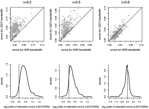
Figure 3: Summary of simulation comparison between ${\widehat{h}}_{\tau\mathrm{HDR}}$ and ${\widehat{h}}_{\mathrm{LSCV}}$ for $\tau=0.2,0.5$ and $0.8$ and 250 samples of size 1000 generated from Density 4 of Marron and Wand (1992). The upper panels are scatterplots of the errors $\mu_{f}(\widehat{R}_{h,\tau}\triangle R_{\tau})$ for $h={\widehat{h}}_{\mathrm{LSCV}}$ on the vertical axes and $h={\widehat{h}}_{\tau\mathrm{HDR}}$ on the horizontal axes. The lower panels are kernel density estimates of $\log_{10}((\mbox{error for }h={\widehat{h}}_{\tau\mathrm{HDR}})/(\mbox{error for }h={\widehat{h}}_{\mathrm{LSCV}}))$.

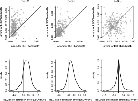
Figure 4: Summary of simulation comparison between ${\widehat{h}}_{\tau\mathrm{HDR}}$ and ${\widehat{h}}_{\mathrm{LSCV}}$ for $\tau=0.2,0.5$ and $0.8$ and 250 samples of size 100,000 generated from Density 4 of Marron and Wand (1992). The upper panels are scatterplots of the errors $\mu_{f}(\widehat{R}_{h,\tau}\triangle R_{\tau})$ for $h={\widehat{h}}_{\mathrm{LSCV}}$ on the vertical axes and $h={\widehat{h}}_{\tau\mathrm{HDR}}$ on the horizontal axes. The lower panels are kernel density estimates of $\log_{10}((\mbox{error for }h={\widehat{h}}_{\tau\mathrm{HDR}})/(\mbox{error for }h={\widehat{h}}_{\mathrm{LSCV}}))$.

We performed similar simulation comparisons for the remaining Densities 1–10 of Marron and Wand (1992). For $n=1000$ the performance of ${\widehat{h}}_{\tau\mathrm{HDR}}$ was better than ${\widehat{h}}_{\mathrm{LSCV}}$ for Densities 1–5; whereas ${\widehat{h}}_{\mathrm{LSCV}}$ did better for Densities 6–10. This suggests that the asymptotics on which ${\widehat{h}}_{\tau\mathrm{HDR}}$ relies have not “kicked in” at $n=1000$ for these more intricate density functions. We suspect that more sophisticated pilot estimation might improve matters for HDR-based bandwidth selection for lower sample sizes. The $n=100\mbox{,}000$ simulations show superior performance of ${\widehat{h}}_{\tau\mathrm{HDR}}$, especially $\tau=0.8$ where it is the “winner” for 9 out of the 10 density functions. The overarching conclusion is that for common density estimation situations ${\widehat{h}}_{\tau\mathrm{HDR}}$ is better than ${\widehat{h}}_{\mathrm{LSCV}}$.

3.3 Application to daily temperature data

We conclude with an application to data on daily maximum temperatures in Melbourne, Australia, for the years 1981–1990. These data were used in Hyndman (1996) to illustrate HDR principles. We revisit them armed with the automatic HDR estimation technology described in Section 3.1. Of interest are the conditional densities of tomorrow’s temperature given today’s temperature is within a fixed interval.

The intervals for the “today’s temperature” values are, in degrees Celsius,

$$[5,10),[10,15),\ldots,[40,45).$$

Figure 5 shows the kernel

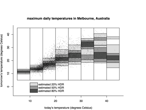
Figure 5: Estimated kernel HDRs for the conditional densities of tomorrow’s temperature given that today’s temperature is in a fixed interval. The bandwidth for each HDR estimate is chosen using the selector described in Section 3.1.

estimates of the 20%, 50% and 80% HDRs with bandwidths chosen using the rule ${\widehat{h}}_{\tau\mathrm{HDR}}$ as detailed in Section 3.1. Some interesting bimodality in “tomorrow’s temperature” is apparent when conditioned on today’s temperature being in the 30–40 degrees Celsius range.

Appendix: Proofs

Proof of Theorem 1

Throughout the proof, it is convenient to write $x_{0}=-\infty$ and $x_{2r+1}=\infty$ and adopt the convention that $x_{0}+a=-\infty$ and $x_{2r+1}+a=\infty$ for all $a\in\mathbb{R}$. Observe that

$$\mu_{f}(\widehat{R}_{h,\tau}\triangle R_{\tau}) = \int_{-\infty}^{\infty}f(x)\bigl{|}\mathbh{1}_{\{\widehat{f}_{h}(x)\geq\widehat{f}_{h,\tau}\}}-\mathbh{1}_{\{f(x)\geq f_{\tau}\}}\bigr{|}\,dx$$

$$= \sum_{j=0}^{r}\int_{x_{2j}}^{x_{2j+1}}f(x)\mathbh{1}_{\{\widehat{f}_{h}(x)\geq\widehat{f}_{h,\tau}\}}\,dx$$

$${}+\sum_{j=1}^{r}\int_{x_{2j-1}}^{x_{2j}}f(x)\mathbh{1}_{\{\widehat{f}_{h}(x)<\widehat{f}_{h,\tau}\}}\,dx,$$

so that

$$\mathbb{E}\{\mu_{f}(\widehat{R}_{h,\tau}\triangle R_{\tau})\} = \sum_{j=0}^{r}\int_{x_{2j}}^{x_{2j+1}}f(x)\mathbb{P}\bigl{(}\widehat{f}_{h}(x)\geq\widehat{f}_{h,\tau}\bigr{)}\,dx$$

$${}+\sum_{j=1}^{r}\int_{x_{2j-1}}^{x_{2j}}f(x)\mathbb{P}\bigl{(}\widehat{f}_{h}(x)<\widehat{f}_{h,\tau}\bigr{)}\,dx.$$

The main idea of the proof is that the dominant contribution to $\mathbb{E}\{\mu_{f}(\widehat{R}_{h,\tau}\triangle R_{\tau})\}$ comes from a union of $2r$ small intervals, one near each $x_{j}$, where $\mathbb{P}(\widehat{f}_{h}(x)\geq\widehat{f}_{h,\tau})$ is close to $1/2$. In each of these intervals, we can represent $\widehat{f}_{h}(x)-\widehat{f}_{h,\tau}$ by a sample mean of independent and identically distributed random variables and a small additional remainder term, and hence apply a normal approximation to deduce the result. For clarity of exposition, we now split the proof into several steps:

Step 1.

As a preliminary step, let $\tilde{f}=f+g$ be another uniformly continuous density, and let $\tilde{f}_{\tau}=f_{\tau}(\tilde{f})$. Writing $\|\cdot\|_{\infty}$ for the supremum norm on the real line, we show that there exists $C\geq 1$ such that for all $\varepsilon>0$ sufficiently small, we have $|\tilde{f}_{\tau}-f_{\tau}|\leq C\varepsilon$ whenever $\|g\|_{\infty}\equiv\|\tilde{f}-f\|_{\infty}\leq\varepsilon$. To see this, let $L=\sum_{j=1}^{r}(x_{2j}-x_{2j-1})$ and choose $C>1+2L\{\frac{1}{4}f_{\tau}\sum_{j=1}^{2r}\frac{1}{|f^{\prime}(x_{j})|}\}^{-1}$. The inverse function theorem [Burkill and Burkill (2002), Theorem 7.51] gives that for $\varepsilon\in\mathbb{R}$ with $|\varepsilon|$ sufficiently small, we can write

$$\{x\dvtx f(x)\geq f_{\tau}+\varepsilon\}=\bigcup_{j=1}^{r}[x_{2j-1}+\delta_{\varepsilon,2j-1},x_{2j}-\delta_{\varepsilon,2j}]$$

with $\delta_{\varepsilon,j}=\frac{\varepsilon}{|f^{\prime}(x_{j})|}+O(\varepsilon^{2})$ as $\varepsilon\rightarrow 0$. It follows that when $\varepsilon>0$ is sufficiently small, and $\|g\|_{\infty}\leq\varepsilon$, we have

$$\int_{-\infty}^{\infty}\tilde{f}(x)\mathbh{1}_{\{\tilde{f}(x)\geq f_{\tau}-C\varepsilon\}}\,dx$$

$$\qquad\geq\int_{-\infty}^{\infty}\{f(x)-\varepsilon\}\mathbh{1}_{\{f(x)\geq f_{\tau}-(C-1)\varepsilon\}}\,dx$$

$$\qquad=1-\tau+\sum_{j=1}^{r}\int_{x_{2j-1}+\delta_{-\varepsilon(C-1),2j-1}}^{x_{2j-1}}f(x)\,dx$$

$$\qquad\quad{}+\sum_{j=1}^{r}\int_{x_{2j}}^{x_{2j}-\delta_{-\varepsilon(C-1),2j}}f(x)\,dx$$

$$\qquad\quad{}-\varepsilon\sum_{j=1}^{r}\bigl{\{}x_{2j}-\delta_{-\varepsilon(C-1),2j}-\bigl{(}x_{2j-1}+\delta_{-\varepsilon(C-1),2j-1}\bigr{)}\bigr{\}}$$

$$\qquad\geq 1-\tau+\frac{1}{4}(C-1)\varepsilon f_{\tau}\sum_{j=1}^{2r}\frac{1}{|f^{\prime}(x_{j})|}-2\varepsilon L>1-\tau.$$

Thus $\tilde{f}_{\tau}\geq f_{\tau}-C\varepsilon$. A very similar argument yields the upper bound $\tilde{f}_{\tau}\leq f_{\tau}+C\varepsilon$, and this completes Step 1.

Now, for $\delta>0$ small enough that $f$ has two continuous derivatives in $I_{\delta}\equiv\bigcup_{j=1}^{r}[x_{2j-1}-\delta,x_{2j}+\delta]$, let $\|\cdot\|_{I_{\delta},\infty}$ denote the supremum norm restricted to $I_{\delta}$. It will be helpful in Step 4 to note that a small modification of the above argument may be used to prove that if $\|g\|_{\infty}$ and $\|g^{\prime}\|_{I_{\delta},\infty}$ are sufficiently small, and if

$$\sum_{j=1}^{r}\int_{x_{2j-1}-\delta}^{x_{2j}+\delta}|g(x)|\,dx=O\Biggl{(}\sum_{j=1}^{2r}|g(x_{j})|\Biggr{)}$$

as $\sum_{j=1}^{2r}|g(x_{j})|\rightarrow 0$, then $\tilde{f}_{\tau}-f_{\tau}=O(\sum_{j=1}^{2r}|g(x_{j})|)$ as $\sum_{j=1}^{2r}|g(x_{j})|\rightarrow 0$.

Step 2.

We show that for each fixed $\delta>0$,

$$\sum_{j=0}^{r}\int_{x_{2j}+\delta}^{x_{2j+1}-\delta}f(x)\mathbb{P}\bigl{(}\widehat{f}_{h}(x)\geq\widehat{f}_{h,\tau}\bigr{)}\,dx$$

(1)

$$\qquad{}+\sum_{j=1}^{r}\int_{x_{2j-1}+\delta}^{x_{2j}-\delta}f(x)\mathbb{P}\bigl{(}\widehat{f}_{h}(x)<\widehat{f}_{h,\tau}\bigr{)}\,dx=o(n^{-1})$$

as $n\rightarrow\infty$. In fact, we claim (and it will be straightforward to see) that the error term is of the stated order uniformly for $h\in[h^{-},h^{+}]$. Indeed, we make a similar claim for every error term in each expression below where the bandwidth $h$ appears, but we do not repeat this assertion in future occurrences. As in Step 1, observe that under (A1), if $\delta>0$ is sufficiently small, then there exists $\varepsilon>0$ such that $f(x)\leq f_{\tau}-\varepsilon$ for $x\in\bigcup_{j=0}^{r}[x_{2j}+\delta,x_{2j+1}-\delta]$ and $f(x)\geq f_{\tau}+\varepsilon$ for $x\in\bigcup_{j=1}^{r}[x_{2j-1}+\delta,x_{2j}-\delta]$. By reducing $\delta>0$ if necessary, for $x\in\bigcup_{j=0}^{r}[x_{2j}+\delta,x_{2j+1}-\delta]$,

$$\mathbb{P}\bigl{(}\widehat{f}_{h}(x)\geq\widehat{f}_{h,\tau}\bigr{)} \leq \mathbb{P}\bigl{(}\widehat{f}_{h}(x)-f(x)-(\widehat{f}_{h,\tau}-f_{\tau})\geq\varepsilon\bigr{)}$$

$$\leq \mathbb{P}(\|\widehat{f}_{h}-f\|_{\infty}\geq\varepsilon/2)+\mathbb{P}(|\widehat{f}_{h,\tau}-f_{\tau}|\geq\varepsilon/2)$$

$$\leq 2\mathbb{P}\biggl{(}\|\widehat{f}_{h}-f\|_{\infty}\geq\frac{\varepsilon}{2C}\biggr{)},$$

where we have used the result of Step 1 in the last inequality, and $C$ is the constant defined in that step. A very similar argument yields the same upper bound for $\mathbb{P}(\widehat{f}_{h}(x)<\widehat{f}_{h,\tau})$ when $x\in\bigcup_{j=1}^{r}[x_{2j-1}+\delta,x_{2j}-\delta]$. Now, since $f$ is uniformly continuous under (A1),

$$\|\mathbb{E}(\widehat{f}_{h})-f\|_{\infty}=\sup_{x\in\mathbb{R}}\biggl{|}\int_{-\infty}^{\infty}K(z)\{f(x-hz)-f(x)\}\,dz\biggr{|}\rightarrow 0$$ (3)

as $n\rightarrow\infty$. The inequality (2), together with the observation (3) on the bias of $\widehat{f}_{h}$, yields that for $n$ sufficiently large,

$$\sum_{j=0}^{r}\int_{x_{2j}+\delta}^{x_{2j+1}-\delta}f(x)\mathbb{P}\bigl{(}\widehat{f}_{h}(x)\geq\widehat{f}_{h,\tau}\bigr{)}\,dx$$

$$\quad{}+\sum_{j=1}^{r}\int_{x_{2j-1}+\delta}^{x_{2j}-\delta}f(x)\mathbb{P}\bigl{(}\widehat{f}_{h}(x)<\widehat{f}_{h,\tau}\bigr{)}\,dx$$

$$\qquad\leq 2\mathbb{P}\biggl{(}\|\widehat{f}_{h}-\mathbb{E}(\widehat{f}_{h})\|_{\infty}\geq\frac{\varepsilon}{4C}\biggr{)}$$

$$\qquad\leq\exp(-c_{1}nh\varepsilon^{2})$$

for some $c_{1}>0$. Here, the final inequality is an application of Corollary 2.2 of Giné and Guillou (2002) (a consequence of Talagrand’s inequality) to the Vapnik–Cervonenkis class of functions $\{K((x-\cdot)/h)\dvtx x\in\mathbb{R},h>0\}$ [cf. Dudley (1999), Theorems 4.2.1 and 4.2.4]. Equation (2) follows immediately, and this completes the proof of Step 2.

Step 3.

We show that (2) continues to hold if $\delta$ is replaced by a sequence $(\delta_{n})$ converging to zero, provided that $\delta_{n}\rightarrow 0$ slowly enough that $n^{1/4}\delta_{n}\rightarrow\infty$ and $(h^{+})^{2}=o(\delta_{n})$. In order to complete the proof of Step 3, it suffices to show that there exists $\delta>0$ such that

$$E(\delta,\delta_{n}) \equiv \sum_{j=1}^{r}\int_{x_{2j-1}-\delta}^{x_{2j-1}-\delta_{n}}\mathbb{P}\bigl{(}\widehat{f}_{h}(x)\geq\widehat{f}_{h,\tau}\bigr{)}\,dx$$

$${}+\sum_{j=1}^{r}\int_{x_{2j-1}+\delta_{n}}^{x_{2j-1}+\delta}\mathbb{P}\bigl{(}\widehat{f}_{h}(x)<\widehat{f}_{h,\tau}\bigr{)}\,dx\sum_{j=1}^{r}\int_{x_{2j}-\delta}^{x_{2j}-\delta_{n}}\mathbb{P}\bigl{(}\widehat{f}_{h}(x)<\widehat{f}_{h,\tau}\bigr{)}\,dx$$

$${}+\sum_{j=1}^{r}\int_{x_{2j}+\delta_{n}}^{x_{2j}+\delta}\mathbb{P}\bigl{(}\widehat{f}_{h}(x)\geq\widehat{f}_{h,\tau}\bigr{)}\,dx=o(n^{-1}).$$

We may assume $\delta>0$ is small enough that $f$ has two continuous derivatives in $I_{\delta}$. This enables a straightforward modification to the argument in (3) using a Taylor expansion, leading to

$$\|\mathbb{E}(\widehat{f}_{h})-f\|_{I_{\delta},\infty}=O(h^{2}).$$ (4)

Now there exists a constant $c_{2}>0$ small enough that if we take $\varepsilon_{n}=c_{2}\delta_{n}$, then we have $|f(x)-f_{\tau}|\geq\varepsilon_{n}$ when $\min_{j}|x-x_{j}|\geq\delta_{n}$. Moreover, $(h^{+})^{2}=o(\varepsilon_{n})$, so that for $n$ sufficiently large, the same argument as in Step 2 yields

$$E(\delta,\delta_{n}) \leq 2\mathbb{P}\biggl{(}\|\widehat{f}_{h}-\mathbb{E}(\widehat{f}_{h})\|_{\infty}\geq\frac{\varepsilon_{n}}{4C}\biggr{)}$$

$$\leq \exp(-c_{1}nh\varepsilon_{n}^{2})=o(n^{-1}).$$

This completes the proof of Step 3.

Step 4.

We seek asymptotic expansions for $\mathbb{E}(\widehat{f}_{h,\tau})$ and $\operatorname{Var}(\widehat{f}_{h,\tau})$. To this end, for uniformly continuous densities $\tilde{f}=f+g$ that are twice continuously differentiable in $I_{\delta}$, and for $y\in(0,\infty)$, we define

$$\psi(\tilde{f},y)=\int_{-\infty}^{\infty}\tilde{f}(x)\mathbh{1}_{\{\tilde{f}(x)\geq y\}}\,dx.$$

The reason for making this definition is that by examining the behavior of $\psi$ under small changes of its arguments from $(f,f_{\tau})$, we will be able to study the difference $\widehat{f}_{h,\tau}-f_{\tau}$ in (4) below. First, for $\varepsilon>0$ sufficiently small,

$$\Biggl{|}\psi(f,f_{\tau}+\varepsilon)-\psi(f,f_{\tau})+\varepsilon f_{\tau}\sum_{j=1}^{2r}\frac{1}{|f^{\prime}(x_{j})|}\Biggr{|}$$

$$\qquad=\Biggl{|}-\int_{-\infty}^{\infty}f(x)\mathbh{1}_{\{f_{\tau}\leq f(x)<f_{\tau}+\varepsilon\}}\,dx+\varepsilon f_{\tau}\sum_{j=1}^{2r}\frac{1}{|f^{\prime}(x_{j})|}\Biggr{|}$$

$$\qquad=\Biggl{|}-\sum_{j=1}^{r}\biggl{\{}\int_{x_{2j-1}}^{x_{2j-1}+\delta_{\varepsilon,2j-1}}f(x)\,dx$$ (5)

$$\hskip 75.7pt{}+\int_{x_{2j}-\delta_{\varepsilon,2j}}^{x_{2j}}f(x)\,dx\biggr{\}}+\varepsilon f_{\tau}\sum_{j=1}^{2r}\frac{1}{|f^{\prime}(x_{j})|}\Biggr{|}$$

$$\qquad=O(\varepsilon^{2})$$

as $\varepsilon\searrow 0$. A very similar argument shows that the error term is of the same order as $\varepsilon\nearrow 0$.

Observe that when $\|g\|_{\infty}$ and $\|g^{\prime}\|_{I_{\delta},\infty}$ are sufficiently small, $\tilde{f}$ has a nonzero derivative in a neighborhood of each $x_{j}$. It follows that for sufficiently small values of $\|g\|_{\infty}+\|g^{\prime}\|_{I_{\delta},\infty}$, we can write

$$\{x\dvtx\tilde{f}(x)\geq\tilde{f}_{\tau}\}=\bigcup_{j=1}^{r}[x_{2j-1}+\delta_{\varepsilon,2j-1}+\eta_{2j-1},x_{2j}-\delta_{\varepsilon,2j}-\eta_{2j}],$$

where $\varepsilon=\tilde{f}_{\tau}-f_{\tau}$. Moreover, provided that

$$\sum_{j=1}^{r}\int_{x_{2j-1}-\delta}^{x_{2j}+\delta}|g(x)|\,dx=O\Biggl{(}\sum_{j=1}^{2r}|g(x_{j})|\Biggr{)}$$

and $\sum_{j=1}^{2r}|g(x_{j})|=O(\min_{j}|g(x_{j})|)$ as $\sum_{j=1}^{2r}|g(x_{j})|+\|g^{\prime}\|_{I_{\delta},\infty}\rightarrow 0$, we have that $\eta_{j}=\frac{-g(x_{j})}{|f^{\prime}(x_{j})|}+O(|g(x_{j})|\|g^{\prime}\|_{I_{\delta},\infty})$ as $\sum_{j=1}^{2r}|g(x_{j})|+\|g^{\prime}\|_{I_{\delta},\infty}\rightarrow 0$. Thus we can write

$$\Biggl{|}\psi(\tilde{f},\tilde{f}_{\tau})-\psi(f,\tilde{f}_{\tau})-f_{\tau}\sum_{j=1}^{2r}\frac{g(x_{j})}{|f^{\prime}(x_{j})|}-\sum_{j=1}^{r}\int_{x_{2j-1}}^{x_{2j}}g(x)\,dx\Biggr{|}$$

$$\qquad\leq\Biggl{|}\int_{-\infty}^{\infty}f(x)\bigl{(}\mathbh{1}_{\{\tilde{f}(x)\geq\tilde{f}_{\tau}\}}-\mathbh{1}_{\{f(x)\geq\tilde{f}_{\tau}\}}\bigr{)}\,dx-f_{\tau}\sum_{j=1}^{2r}\frac{g(x_{j})}{|f^{\prime}(x_{j})|}\Biggr{|}$$

$$\qquad\quad{}+\biggl{|}\int_{-\infty}^{\infty}g(x)\bigl{(}\mathbh{1}_{\{\tilde{f}(x)\geq\tilde{f}_{\tau}\}}-\mathbh{1}_{\{f(x)\geq f_{\tau}\}}\bigr{)}\,dx\biggr{|}$$

$$\qquad=\Biggl{|}\Biggl{\{}f_{\tau}+O\Biggl{(}\sum_{j=1}^{2r}|g(x_{j})|\Biggr{)}\Biggr{\}}\sum_{j=1}^{2r}\Biggl{\{}\frac{g(x_{j})}{|f^{\prime}(x_{j})|}+O(|g(x_{j})|\|g^{\prime}\|_{I_{\delta},\infty})\Biggr{\}}$$

$$\hskip 233.0pt{}-f_{\tau}\sum_{j=1}^{2r}\frac{g(x_{j})}{|f^{\prime}(x_{j})|}\Biggr{|}$$

$$\qquad\quad{}+O\Biggl{\{}\Biggl{(}\sum_{j=1}^{2r}|g(x_{j})|\Biggr{)}^{2}\Biggr{\}}$$

$$\qquad=O\Biggl{\{}\Biggl{(}\sum_{j=1}^{2r}|g(x_{j})|\Biggr{)}^{2}+\|g^{\prime}\|_{I_{\delta},\infty}\sum_{j=1}^{2r}|g(x_{j})|\Biggr{\}}$$

as $\sum_{j=1}^{2r}|g(x_{j})|+\|g^{\prime}\|_{I_{\delta},\infty}\rightarrow 0$. Assuming that $\psi(\tilde{f},\tilde{f}_{\tau})=1-\tau$ and that the above conditions on $g$ hold, we have from (4) and (4) that

$$\qquad 0 = \psi(\tilde{f},\tilde{f}_{\tau})-\psi(f,f_{\tau})$$

$$= \psi(\tilde{f},\tilde{f}_{\tau})-\psi(f,\tilde{f}_{\tau})+\psi(f,\tilde{f}_{\tau})-\psi(f,f_{\tau})$$

$$= -\{\tilde{f}_{\tau}-f_{\tau}\}f_{\tau}\sum_{j=1}^{2r}\frac{1}{|f^{\prime}(x_{j})|}+f_{\tau}\sum_{j=1}^{2r}\frac{g(x_{j})}{|f^{\prime}(x_{j})|}+\sum_{j=1}^{r}\int_{x_{2j-1}}^{x_{2j}}g(x)\,dx$$

$${}+O\Biggl{\{}\Biggl{(}\sum_{j=1}^{2r}|g(x_{j})|\Biggr{)}^{2}+\|g^{\prime}\|_{I_{\delta},\infty}\sum_{j=1}^{2r}|g(x_{j})|\Biggr{\}}$$

as $\sum_{j=1}^{2r}|g(x_{j})|+\|g^{\prime}\|_{I_{\delta},\infty}\rightarrow 0$.

We want to apply (4) with $\tilde{f}=\widehat{f}_{h}$, so that $g=\widehat{f}_{h}-f$. In order to do this, we must recall observation (3) on the bias of $\widehat{f}_{h}$, and the fact that $\|\widehat{f}_{h}-\mathbb{E}(\widehat{f}_{h})\|_{\infty}=O_{\mathrm{a.s.}}(\frac{\sqrt{\log 1/h}}{(nh)^{1/2}})$ from an application of Corollary 2.2 of Giné and Guillou (2002). It follows that $\|\widehat{f}_{h}-f\|_{\infty}\stackrel{{\scriptstyle\mathrm{a.s.}}}{{\rightarrow}}0$. Similarly, $\|\mathbb{E}(\widehat{f}_{h}^{\prime})-f^{\prime}\|_{I_{\delta},\infty}=O(h^{2})$, and a further application of Corollary 2.2 of Giné and Guillou (2002) gives $\|\widehat{f}_{h}^{\prime}-\mathbb{E}(\widehat{f}_{h}^{\prime})\|_{I_{\delta},\infty}=O_{\mathrm{a.s.}}(\frac{\sqrt{\log 1/h}}{(nh^{3})^{1/2}})$. Thus $\|\widehat{f}_{h}^{\prime}-f^{\prime}\|_{I_{\delta},\infty}\stackrel{{\scriptstyle\mathrm{a.s.}}}{{\rightarrow}}0$. This in turn implies that with probability one, for $n$ sufficiently large, $\widehat{f}_{h,\tau}$ is the unique solution to $\psi(\widehat{f}_{h},\widehat{f}_{h,\tau})=1-\tau$, or equivalently $\int\widehat{f}_{h}(x)\mathbh{1}_{\{\widehat{f}_{h}(x)\geq\widehat{f}_{h,\tau}\}}\,dx=1-\tau$, as claimed in Section 2. It remains to note that

$$\frac{\sum_{j=1}^{r}\int_{x_{2j-1}-\delta}^{x_{2j}+\delta}|\widehat{f}_{h}(x)-f(x)|\,dx}{\sum_{j=1}^{2r}|\widehat{f}_{h}(x_{j})-f(x_{j})|}=O_{p}(1)$$

and

$$\frac{\sum_{j=1}^{2r}|\widehat{f}_{h}(x_{j})-f(x_{j})|}{\min_{j}|\widehat{f}_{h}(x_{j})-f(x_{j})|}=O_{p}(1).$$

It follows that we can now substitute $g=\widehat{f}_{h}-f$ in (4) to deduce that

$$\widehat{f}_{h,\tau}-f_{\tau} = \Biggl{\{}\sum_{j=1}^{2r}\frac{1}{|f^{\prime}(x_{j})|}\Biggr{\}}^{-1}\Biggl{\{}\sum_{j=1}^{2r}\frac{\widehat{f}_{h}(x_{j})-f(x_{j})}{|f^{\prime}(x_{j})|}$$

$$\hskip 84.4pt{}+\frac{1}{f_{\tau}}\sum_{j=1}^{r}\int_{x_{2j-1}}^{x_{2j}}\widehat{f}_{h}(x)-f(x)\,dx\Biggr{\}}$$

$${}+O_{p}\biggl{(}\frac{\sqrt{\log(1/h)}}{nh^{2}}+\frac{h^{1/2}\sqrt{\log(1/h)}}{n^{1/2}}+h^{4}\biggr{)}.$$

Equation (4) shows that we can write the difference $\widehat{f}_{h,\tau}-f_{\tau}$ as a sample mean of independent and identically distributed random variables and a small additional remainder term. Notice from the bandwidth condition on $h^{-}$ in (A2) that $\frac{\sqrt{\log(1/h)}}{nh^{2}}=o(h^{2})$. Next, observe that

$$\sum_{j=1}^{2r}\frac{\mathbb{E}\{\widehat{f}_{h}(x_{j})\}-f(x_{j})}{|f^{\prime}(x_{j})|}+\frac{1}{f_{\tau}}\sum_{j=1}^{r}\int_{x_{2j-1}}^{x_{2j}}\mathbb{E}\{\widehat{f}_{h}(x)\}-f(x)\,dx$$

$$\qquad=D_{1}\sum_{j=1}^{2r}\frac{1}{|f^{\prime}(x_{j})|}h^{2}+o(h^{2}),$$

where $D_{1}$ is given in (2). Thus, in order to prove that

$$\mathbb{E}(\widehat{f}_{h,\tau})=f_{\tau}+D_{1}h^{2}+o(h^{2}),$$ (9)

it suffices by (4) and Step 1 to show that for any $\eta>0$,

$$\mathbb{E}\bigl{(}|\widehat{f}_{h,\tau}-f_{\tau}-D_{1}h^{2}|\mathbh{1}_{\{\sum_{j=1}^{2r}|\widehat{f}_{h}(x_{j})-f(x_{j})|+\|\widehat{f}_{h}^{\prime}-f^{\prime}\|_{I_{\delta},\infty}>\eta\}}\bigr{)}=o(h^{2}).$$

But this follows by Cauchy–Schwarz, because Step 1 may be used to show that $\mathbb{E}(\widehat{f}_{h,\tau}^{2})=O(1)$, and also

$$\mathbb{P}\Biggl{(}\sum_{j=1}^{2r}|\widehat{f}_{h}(x_{j})-f(x_{j})|>\eta/2\Biggr{)}+\mathbb{P}(\|\widehat{f}_{h}^{\prime}-f^{\prime}\|_{I_{\delta},\infty}>\eta/2)=o(n^{-1}).$$

We therefore deduce (9).

In a very similar way, we can also use (4) and the fact that

$$\sum_{j=1}^{2r}\frac{\operatorname{Var}\{\widehat{f}_{h}(x_{j})\}}{f^{\prime}(x_{j})^{2}}=\frac{D_{2}}{nh}\Biggl{\{}\sum_{j=1}^{2r}\frac{1}{|f^{\prime}(x_{j})|}\Biggr{\}}^{2}+o\biggl{(}\frac{1}{nh}\biggr{)},$$

where $D_{2}$ is given in (2), to deduce that

$$\operatorname{Var}(\widehat{f}_{h,\tau})=\frac{D_{2}}{nh}+o\biggl{(}\frac{1}{nh}\biggr{)}.$$ (10)

Step 5.

We can use the results of Step 4 to shrink the region of interest still further. From the result of Step 3 we can write

$$\mathbb{E}\{\mu_{f}(\widehat{R}_{h,\tau}\triangle R_{\tau})\}$$

$$\qquad=\sum_{j=1}^{r}\int_{x_{2j-1}-\delta_{n}}^{x_{2j-1}+\delta_{n}}f(x)\bigl{|}\mathbb{P}\bigl{(}\widehat{f}_{h}(x)<\widehat{f}_{h,\tau}\bigr{)}-\mathbh{1}_{\{x<x_{2j-1}\}}\bigr{|}\,dx$$

$$\qquad\quad{}+\sum_{j=1}^{r}\int_{x_{2j}-\delta_{n}}^{x_{2j}+\delta_{n}}f(x)\bigl{|}\mathbb{P}\bigl{(}\widehat{f}_{h}(x)<\widehat{f}_{h,\tau}\bigr{)}-\mathbh{1}_{\{x\geq x_{2j}\}}\bigr{|}\,dx+o(n^{-1})$$

$$\qquad=\frac{f_{\tau}}{(nh)^{1/2}}\sum_{j=1}^{r}\int_{-(nh)^{1/2}\delta_{n}}^{(nh)^{1/2}\delta_{n}}\bigl{|}\mathbb{P}\bigl{(}\widehat{f}_{h}\bigl{(}x_{2j-1}+(nh)^{-1/2}t\bigr{)}<\widehat{f}_{h,\tau}\bigr{)}-\mathbh{1}_{\{t<0\}}\bigr{|}$$

$$\qquad\quad{}+\bigl{|}\mathbb{P}\bigl{(}\widehat{f}_{h}\bigl{(}x_{2j}+(nh)^{-1/2}t\bigr{)}<\widehat{f}_{h,\tau}\bigr{)}-\mathbh{1}_{\{t\geq 0\}}\bigr{|}\,dt+o(n^{-1}).$$

For brevity, we write $x_{j}^{t}=x_{j}+(nh)^{-1/2}t$. Now, for each $j=1,\ldots,2r$, we see that for $n$ sufficiently large, $\mathbb{E}\{\widehat{f}_{h}(x_{j}^{t})-\widehat{f}_{h,\tau}\}$ is a strictly monotone function of $t\in[-(nh)^{1/2}\delta_{n},(nh)^{1/2}\delta_{n}]$, with a unique zero $t_{j}^{*}$, say. Moreover,

$$t_{j}^{*}=\bigl{\{}D_{1}-\tfrac{1}{2}\mu_{2}(K)f^{\prime\prime}(x_{j})\bigr{\}}\{f^{\prime}(x_{j})\}^{-1}n^{1/2}h^{5/2}\{1+o(1)\}.$$

Fix a sequence $(t_{n})$ diverging to infinity and let $I_{j}^{n}=[-(nh)^{1/2}\delta_{n},(nh)^{1/2}\delta_{n}]\setminus[t_{j}^{*}-t_{n},t_{j}^{*}+t_{n}]$. We claim that

$$\sum_{j=1}^{r}\biggl{\{}\int_{I_{2j-1}^{n}}\bigl{|}\mathbb{P}\bigl{(}\widehat{f}_{h}(x_{2j-1}^{t})<\widehat{f}_{h,\tau}\bigr{)}-\mathbh{1}_{\{t<0\}}\bigr{|}\,dt$$

(12)

$$\hskip 26.6pt{}+\int_{I_{2j}^{n}}\bigl{|}\mathbb{P}\bigl{(}\widehat{f}_{h}(x_{2j}^{t})<\widehat{f}_{h,\tau}\bigr{)}-\mathbh{1}_{\{t\geq 0\}}\bigr{|}\,dt\biggr{\}}\rightarrow 0$$

as $n\rightarrow\infty$. Now there exists $c_{3}>0$ such that for all $t\in\bigcup_{j=1}^{2r}I_{j}^{n}$ and $n$ sufficiently large, we have $|\mathbb{E}\{\widehat{f}_{h}(x_{j}^{t})-\widehat{f}_{h,\tau}\}|\geq c_{3}(nh)^{-1/2}t_{n}$. Thus there exists $c_{4}>0$ such that for all $n$ sufficiently large,

$$\bigl{|}\mathbb{P}\bigl{(}\widehat{f}_{h}(x_{2j-1}^{t})<\widehat{f}_{h,\tau}\bigr{)}-\mathbh{1}_{\{t<0\}}\bigr{|}$$

$$\qquad\leq\mathbb{P}\biggl{(}\biggl{|}\frac{\widehat{f}_{h}(x_{2j-1}^{t})-\mathbb{E}\{\widehat{f}_{h}(x_{2j-1}^{t})\}}{\operatorname{Var}^{1/2}\{\widehat{f}_{h}(x_{2j-1}^{t})\}}\biggr{|}\geq c_{4}t_{n}\biggr{)}$$

$$\qquad\quad{}+\mathbb{P}\biggl{(}\biggl{|}\frac{\widehat{f}_{h,\tau}-\mathbb{E}(\widehat{f}_{h,\tau})}{\operatorname{Var}^{1/2}(\widehat{f}_{h,\tau})}\biggr{|}\geq c_{4}t_{n}\biggr{)}\rightarrow 0,$$

uniformly for $t\in\bigcup_{j=1}^{r}I_{2j-1}^{n}$. Since also $|\mathbb{P}(\widehat{f}_{h}(x_{2j}^{t})<\widehat{f}_{h,\tau})-\mathbh{1}_{\{t\geq 0\}}|\rightarrow 0$ uniformly for $t\in\bigcup_{j=1}^{r}I_{2j}^{n}$, we deduce (5).

Step 6.

We also require an asymptotic expansion for $\operatorname{Cov}(\widehat{f}_{h}(x_{j}^{t}),\widehat{f}_{h,\tau})$, for $t\in[t_{j}^{*}-t_{n},t_{j}^{*}+t_{n}]$. In fact, provided $(t_{n})$ diverges sufficiently slowly, we have

$$\operatorname{Cov}(\widehat{f}_{h}(x_{j}^{t}),\widehat{f}_{h,\tau})=\frac{D_{3,j}}{nh}+o\biggl{(}\frac{1}{nh}\biggr{)},$$

uniformly for $t\in[t_{j}^{*}-t_{n},t_{j}^{*}+t_{n}]$, where $D_{3,j}$ is given at (2). This follows from the expansion (4) and the fact that provided $(t_{n})$ diverges sufficiently slowly,

$$\mathbb{E}\biggl{\{}\frac{1}{h^{2}}K\biggl{(}\frac{x_{j}-X_{1}}{h}\biggr{)}K\biggl{(}\frac{x_{j}^{t}-X_{1}}{h}\biggr{)}\biggr{\}}$$

$$\qquad=\frac{1}{h}\int_{-\infty}^{\infty}K(z)K\biggl{(}\frac{(nh)^{-1/2}t+hz}{h}\biggr{)}f(x_{j}-hz)\,dz$$

$$\qquad=\frac{1}{h}f_{\tau}R(K)+o(h^{-1}),$$

uniformly for $t\in[t_{j}^{*}-t_{n},t_{j}^{*}+t_{n}]$.

Step 7.

To complete the proof of Theorem 1, it suffices by (5) and (5) to show that there exists a sequence $(t_{n})$ diverging to infinity such that

$$\frac{f_{\tau}}{(nh)^{1/2}}\sum_{j=1}^{r}\biggl{\{}\int_{t_{2j-1}^{*}-t_{n}}^{t_{2j-1}^{*}+t_{n}}\bigl{|}\mathbb{P}\bigl{(}\widehat{f}_{h}(x_{2j-1}^{t})<\widehat{f}_{h,\tau}\bigr{)}-\mathbh{1}_{\{t<0\}}\bigr{|}\,dt$$

$$\hskip 64.4pt{}+\int_{t_{2j}^{*}-t_{n}}^{t_{2j}^{*}+t_{n}}\bigl{|}\mathbb{P}\bigl{(}\widehat{f}_{h}(x_{2j}^{t})<\widehat{f}_{h,\tau}\bigr{)}-\mathbh{1}_{\{t\geq 0\}}\bigr{|}\,dt\biggr{\}}$$

$$\qquad=\sum_{j=1}^{2r}\biggl{[}\frac{B_{1,j}\phi(B_{2,j}n^{1/2}h^{5/2})}{(nh)^{1/2}}+B_{3,j}h^{2}\{2\Phi(B_{2,j}n^{1/2}h^{5/2})-1\}\biggr{]}$$

$$\qquad\quad{}+o\biggl{(}\frac{1}{(nh)^{1/2}}+h^{2}\biggr{)}.$$

For $i=1,\ldots,n$, let $Z_{ni}(x)=h^{-1}K(\frac{x-X_{i}}{h})$ and let $\bar{Y}_{n}=n^{-1}\sum_{i=1}^{n}Y_{ni}$, where

$$Y_{ni} = Z_{ni}(x_{j}^{t})-f_{\tau}-\Biggl{\{}\sum_{k=1}^{2r}\frac{1}{|f^{\prime}(x_{k})|}\Biggr{\}}^{-1}\Biggl{[}\sum_{k=1}^{2r}\frac{Z_{ni}(x_{k})-f(x_{k})}{|f^{\prime}(x_{k})|}$$

$$\hskip 154.6pt{}+\frac{1}{f_{\tau}}\sum_{k=1}^{r}\int_{x_{2k-1}}^{x_{2k}}Z_{ni}(x)-f(x)\,dx\Biggr{]}.$$

By (4) and (4), we can write $\widehat{f}_{h}(x_{j}^{t})-\widehat{f}_{h,\tau}=\bar{Y}_{n}+R_{n}$, where $R_{n}-\mathbb{E}(R_{n})=o_{p}\{(nh)^{-1/2}\}$. Since $\operatorname{Var}(\bar{Y}_{n})=O\{(nh)^{-1}\}$ uniformly for $t\in[t_{j}^{*}-t_{n},t_{j}^{*}+t_{n}]$, we choose $(t_{n})$ to diverge to infinity so slowly that:

• $\mathbb{P}(\frac{|R_{n}-\mathbb{E}(R_{n})|}{\operatorname{Var}^{1/2}(\bar{Y}_{n})}>\frac{1}{t_{n}^{2}})\leq\frac{1}{t_{n}^{2}}$, uniformly for $t\in[t_{j}^{*}-t_{n},t_{j}^{*}+t_{n}]$;

• $(nh)\operatorname{Var}(\bar{Y}_{n})=R(K)f_{\tau}-2D_{3,j}+D_{2}+o(t_{n}^{-1})$, uniformly for $t\in[t_{j}^{*}-t_{n},t_{j}^{*}+t_{n}]$;

• $\mathbb{E}(\bar{Y}_{n}+R_{n})=\{(nh)^{-1/2}tf^{\prime}(x_{j})+D_{4}h^{2}\}\{1+o(t_{n}^{-1})\}$, uniformly for $t\in[t_{j}^{*}-t_{n},t_{j}^{*}+t_{n}]$, where $D_{4}=\frac{1}{2}\mu_{2}(K)f^{\prime\prime}(x_{j})-D_{1}$;

• $t_{n}=o(n^{1/6})$.

Then

$$\mathbb{P}\bigl{(}\widehat{f}_{h}(x_{j}^{t})<\widehat{f}_{h,\tau}\bigr{)}-\Phi\biggl{(}\frac{-tf^{\prime}(x_{j})-D_{4}n^{1/2}h^{5/2}}{\{R(K)f_{\tau}-2D_{3,j}+D_{2}\}^{1/2}}\biggr{)}$$

$$\qquad\leq\mathbb{P}\biggl{(}\frac{|R_{n}-\mathbb{E}(R_{n})|}{\operatorname{Var}^{1/2}(\bar{Y}_{n})}>\frac{1}{t_{n}^{2}}\biggr{)}$$

$$\qquad\quad{}+\mathbb{P}\biggl{(}\frac{\bar{Y}_{n}-\mathbb{E}(\bar{Y}_{n})}{\operatorname{Var}^{1/2}(\bar{Y}_{n})}\leq\frac{-\mathbb{E}(\bar{Y}_{n}+R_{n})}{\operatorname{Var}^{1/2}(\bar{Y}_{n})}+\frac{1}{t_{n}^{2}}\biggr{)}$$

$$\qquad\quad{}-\Phi\biggl{(}\frac{-tf^{\prime}(x_{j})-D_{4}n^{1/2}h^{5/2}}{\{R(K)f_{\tau}-2D_{3,j}+D_{2}\}^{1/2}}\biggr{)}$$

$$\qquad=O\biggl{(}\frac{1}{t_{n}^{2}}+\frac{1}{(nh)^{1/2}}\biggr{)}+\Phi\biggl{(}\frac{-\mathbb{E}(\bar{Y}_{n}+R_{n})}{\operatorname{Var}^{1/2}(\bar{Y}_{n})}\biggr{)}$$

$$\qquad\quad{}-\Phi\biggl{(}\frac{-tf^{\prime}(x_{j})-D_{4}n^{1/2}h^{5/2}}{\{R(K)f_{\tau}-2D_{3,j}+D_{2}\}^{1/2}}\biggr{)}$$

$$\qquad=o(t_{n}^{-1}),$$

uniformly for $t\in[t_{j}^{*}-t_{n},t_{j}^{*}+t_{n}]$. Here we have used the Berry–Esseen inequality to reach the penultimate line. A very similar argument yields a lower bound of the same order. The proof of Step 7, and hence the proof of Theorem 1, is now completed by the observation that

$$\frac{f_{\tau}}{(nh)^{1/2}}\sum_{j=1}^{r}\biggl{\{}\int_{-\infty}^{\infty}\biggl{|}\Phi\biggl{(}\frac{-tf^{\prime}(x_{2j-1})-D_{4}n^{1/2}h^{5/2}}{\{R(K)f_{\tau}-2D_{3,j}+D_{2}\}^{1/2}}\biggr{)}-\mathbh{1}_{\{t<0\}}\biggr{|}$$

$$\hskip 45.7pt\quad{}+\biggl{|}\Phi\biggl{(}\frac{-tf^{\prime}(x_{2j})-D_{4}n^{1/2}h^{5/2}}{\{R(K)f_{\tau}-2D_{3,j}+D_{2}\}^{1/2}}\biggr{)}-\mathbh{1}_{\{t\geq 0\}}\biggr{|}\,dt\biggr{\}}$$

$$\qquad=\sum_{j=1}^{2r}\biggl{[}\frac{B_{1,j}\phi(B_{2,j}n^{1/2}h^{5/2})}{(nh)^{1/2}}+B_{3,j}h^{2}\{2\Phi(B_{2,j}n^{1/2}h^{5/2})-1\}\biggr{]}.$$

Proof of Corollary 2

We may restrict attention to the case where $nh^{5}$ is bounded away from zero and infinity. The important point to note is that under the hypotheses of the corollary, $B_{1,j}$, $B_{2,j}$ and $B_{3,j}$ do not depend on $j$, so we write them as $B_{1}$, $B_{2}$ and $B_{3}$, respectively.

By making the substitution $x=B_{2}n^{1/2}h^{5/2}$, there exist positive constants $a=2B_{1}B_{2}^{1/5}$ and $b=B_{3}/(B_{1}B_{2})$ such that $\lim_{n\rightarrow\infty}n^{2/5}\mathbb{E}\{\mu_{f}(\widehat{R}_{h,\tau}\triangle R_{\tau})\}=au(x)$, where $u(x)=x^{-1/5}\phi(x)+bx^{4/5}\{2\Phi(x)-1\}$. Since $u$ is continuous with $u(x)\rightarrow\infty$ as $x\searrow 0$ and $x\rightarrow\infty$, it attains its minimum in $(0,\infty)$. To show this minimum is unique, it suffices to show that $v(x)$ has a unique zero in $(0,\infty)$, where

$$v(x)=\frac{5x^{6/5}}{\phi(x)}u^{\prime}(x)=-1+\frac{4bx\{2\Phi(x)-1\}}{\phi(x)}+5(2b-1)x^{2}.$$

Now we have

$$v^{\prime}(x) = 2(14b-5)x+\frac{4b(1+x^{2})\{2\Phi(x)-1\}}{\phi(x)},$$

$$v^{\prime\prime}(x) = 2(18b-5)+8bx^{2}+\frac{4b(3x+x^{3})\{2\Phi(x)-1\}}{\phi(x)}.$$

There are therefore two cases to consider: if $b\geq 5/18$, then $v$ is strictly convex, so since $v(0+)=-1$ and $v(x)\rightarrow\infty$ as $x\rightarrow\infty$, we see that $v$ has a unique zero in $(0,\infty)$. On the other hand, if $b<5/18$, then there exists $x^{*}\in(0,\infty)$ such that $v^{\prime\prime}(x)<0$ for $x\in(0,x^{*})$ and $v^{\prime\prime}(x)>0$ for $x\in(x^{*},\infty)$. But if $b<5/18$ then $v^{\prime}(x)<0$, for sufficiently small $x>0$, so from $v(0+)=-1$, it again follows that $v$ has a unique zero.

Write $x_{\min}$ for the unique minimum of $u$ in $(0,\infty)$, and let $c_{\mathrm{opt}}=(x_{\min}/B_{2})^{2/5}$. We conclude that any optimal bandwidth sequence $(h_{\mathrm{opt}})$, in the sense of minimizing $\mathbb{E}\{\mu_{f}(\widehat{R}_{h,\tau}\triangle R_{\tau})\}$, must satisfy $h_{\mathrm{opt}}=c_{\mathrm{opt}}n^{-1/5}\{1+o(1)\}$ as $n\rightarrow\infty$.

Proof of Theorem 3

We require a bound on $|\widehat{x}_{j,h_{0}}-x_{j}|$ for $j=1,\ldots,2r$. To this end, let $\tilde{f}=f+g$ be another density satisfying the same conditions as $f$. From Step 4 of the proof of Theorem 1, we see that for sufficiently small values of $\|g\|_{\infty}+\|g^{\prime}\|_{I_{\delta},\infty}$, there exist precisely $2r$ values $\tilde{x}_{1}<\cdots<\tilde{x}_{2r}$ such that $\tilde{f}(\tilde{x}_{j})=\tilde{f}_{\tau}$. Moreover, provided $\sum_{j=1}^{r}\int_{x_{2j-1}-\delta}^{x_{2j}+\delta}|g(x)|\,dx=O(\sum_{j=1}^{2r}|g(x_{j})|)$ as $\sum_{j=1}^{2r}|g(x_{j})|+\|g^{\prime}\|_{I_{\delta},\infty}\rightarrow 0$, we have $\tilde{x}_{j}-x_{j}=O(|g(x_{j})|)$ as $\sum_{j=1}^{2r}|g(x_{j})|+\|g^{\prime}\|_{I_{\delta},\infty}\rightarrow 0$. Substituting $\tilde{f}=\widehat{f}_{h_{0}}$, so that $g=\widehat{f}_{h_{0}}-f$ and $\tilde{x}_{j}=\widehat{x}_{j,h_{0}}$, we have $|\widehat{x}_{j,h_{0}}-x_{j}|=O_{p}(n^{-2/5})$.

It follows that $\widehat{D}_{1}=D_{1}+O_{p}(n^{-2/9})$, the crucial fact being that $\widehat{f}_{h_{2}}^{\prime\prime}(\widehat{x}_{j,h_{0}})-f^{\prime\prime}(x_{j})=O_{p}(n^{-2/9})$. Similarly, $\widehat{D}_{2}=D_{2}+O_{p}(n^{-2/7})$ and $\widehat{D}_{3,j}=D_{3,j}+O_{p}(n^{-2/7})$ for $j=1,\ldots,2r$. Thus $\widehat{B}_{1,j}=B_{1,j}+O_{p}(n^{-2/7})$, $\widehat{B}_{2,j}=B_{2,j}+O_{p}(n^{-2/9})$ and $\widehat{B}_{3,j}=B_{3,j}+O_{p}(n^{-2/9})$. We deduce that for any $0<c_{1}<c_{2}<\infty$, we have $\widehat{\mathrm{AR}}_{n}(c)=\mathrm{AR}(c)\{1+O_{p}(n^{-2/9})\}$, uniformly for $c\in[c_{1},c_{2}]$, and a standard Taylor expansion argument then gives that $\widehat{c}_{\mathrm{opt}}=c_{\mathrm{opt}}\{1+O_{p}(n^{-2/9})\}$. Both conclusions of the theorem follow immediately.

Proof of Theorem 4

Let $z_{n}=\delta/h_{2}$, where $\delta$ is small enough that $f$ has 12 continuous derivatives in $\bigcup_{j=1}^{2r}[x_{j}-\delta,x_{j}+\delta]$. Under the conditions of the theorem, we may integrate by parts twice and apply a Taylor expansion to obtain

$$|\mathbb{E}\{\widehat{f}_{h_{2}}^{\prime\prime}(x_{j})\}-f^{\prime\prime}(x_{j})| = \biggl{|}\int_{-z_{n}}^{z_{n}}K_{2}(z)\{f^{\prime\prime}(x_{j}-h_{2}z)-f^{\prime\prime}(x_{j})\}\,dz\biggr{|}+o(h_{2}^{10})$$

$$= O(h_{2}^{10}).$$

This expression for the bias can be combined with the standard fact that $\operatorname{Var}\widehat{f}_{h_{2}}^{\prime\prime}(x_{j})=O\{(nh_{2}^{5})^{-1}\}$ and the bound on $|\widehat{x}_{j,h_{0}}-x_{j}|$ from the proof of Theorem 3 to yield $\widehat{f}_{h_{2}}^{\prime\prime}(\widehat{x}_{j,h_{0}})-f^{\prime\prime}(x_{j})=O_{p}(n^{-2/5})$. Similar computations give $\widehat{f}_{h_{1}}^{\prime}(\widehat{x}_{j,h_{0}})-f^{\prime}(x_{j})=O_{p}(n^{-2/5})$. The rest of the proof mirrors the proof of Theorem 3.

References

• (1) Baíllo, A. (2003). Total error in a plug-in estimator of level sets. Statist. Probab. Lett. 65 411–417. \MR2039885
• (2) Baíllo, A., Cuesta-Albertos, J. A. and Cuevas, A. (2001). Convergence rates in nonparametric estimation of level sets. Statist. Probab. Lett. 53 27–35. \MR1843338
• (3) Bowman, A. W. (1984). An alternative method of cross-validation for the smoothing of density estimates. Biometrika 71 353–360. \MR0767163
• (4) Burkill, J. C. and Burkill, H. (2002). A Second Course in Mathematical Analysis. Cambridge Univ. Press, Cambridge. \MR1962361
• (5) Cadre, B. (2006). Kernel estimation of density level sets. J. Multivariate Anal. 97 999–1023. \MR2256570
• (6) Dudley, R. M. (1999). Uniform Central Limit Theorems. Cambridge Studies in Advanced Mathematics 63. Cambridge Univ. Press, Cambridge. \MR1720712
• (7) Giné, E. and Guillou, A. (2002). Rates of strong uniform consistency for multivariate kernel density estimators. Ann. Inst. H. Poincaré Probab. Statist. 38 907–921. \MR1955344
• (8) González-Manteiga, W., Sanchéz-Sellero, C. and Wand, M. P. (1996). Accuracy of binned kernel functional approximations. Comput. Statist. Data Anal. 22 1–16. \MR1394540
• (9) Hartigan, J. A. (1987). Estimation of a convex density contour in two dimensions. J. Amer. Statist. Assoc. 82 267–270. \MR0883354
• (10) Hyndman, R. J. (1996). Computing and graphing highest density regions. Amer. Statist. 50 120–126.
• (11) Hyndman, R. J. (2009). hdrcde 2.12. Highest density regions and conditional density estimation. R package. Available at http://cran.r-project.org.
• (12) Jang, W. (2006). Nonparametric density estimation and clustering in astronomical sky surveys. Comput. Statist. Data Anal. 50 760–774. \MR2207006
• (13) Marron, J. S. and Wand, M. P. (1992). Exact mean integrated squared error. Ann. Statist. 20 712–736. \MR1165589
• (14) Mason, D. M. and Polonik, W. (2009). Asymptotic normality of plug-in level set estimates. Ann. Appl. Probab. 19 1108–1142. \MR2537201
• (15) Müller, D. W. and Sawitzki, G. (1991). Excess mass estimates and tests for multimodality. J. Amer. Statist. Assoc. 86 738–746. \MR1147099
• (16) Park, B. U. and Marron, J. S. (1990). Comparison of data-driven bandwidth selectors. J. Amer. Statist. Assoc. 85 66–72.
• (17) Polonik, W. (1995). Measuring mass concentrations and estimating density contour clusters—an excess mass approach. Ann. Statist. 23 855–881. \MR1345204
• (18) R Development Core Team (2008). R: A language and environment for statistical computing. R Foundation for Statistical Computing, Vienna, Austria. Available at http://www.R-project.org.
• (19) Rigollet, P. and Vert, R. (2009). Optimal rates for plug-in estimators of density level sets. Bernoulli 15 1154–1178.
• (20) Rudemo, M. (1982). Empirical choice of histograms and kernel density estimators. Scand. J. Statist. 9 65–78. \MR0668683
• (21) Sheather, S. J. and Jones, M. C. (1991). A reliable data-based bandwidth selection method for kernel density estimation. J. Roy. Statist. Soc. Ser. B 53 683–690. \MR1125725
• (22) Tsybakov, A. B. (1997). On nonparametric estimation of density level sets. Ann. Statist. 25 948–969. \MR1447735
• (23) Wand, M. P. and Jones, M. C. (1995). Kernel Smoothing. Monographs on Statistics and Applied Probability 60. Chapman and Hall, London. \MR1319818