A Note on the Inverse Problem with LTB Universes

Abstract

The inverse problem with Lemaître-Tolman-Bondi (LTB) universe models is discussed. The LTB solution for the Einstein equations describes the spherically symmetric dust-filled spacetime. The LTB solution has two physical functional degrees of freedom of the radial coordinate. The inverse problem is constructing an LTB model requiring that the LTB model be consistent with selected important observational data. In this paper, we assume that the observer is at the center and consider the distance-redshift relation $D_{\rm A}$ and the redshift-space mass density $\mu$ as the selected important observational data. We give $D_{\rm A}$ and $\mu$ as functions of the redshift $z$. Then, we explicitly show that, for general functional forms of $D_{\rm A}(z)$ and $\mu(z)$, the regular solution does not necessarily exist in the whole redshift domain. We also show that the condition for the existence of the regular solution is satisfied by the distance-redshift relation and the redshift-space mass density in $\Lambda$CDM models. Deriving regular differential equations for the inverse problem with the distance-redshift relation and the redshift-space mass density in $\Lambda$CDM models, we numerically solve them for the case $(\Omega_{\rm M0},\Omega_{\Lambda 0})=(0.3,0.7)$. A set of analytic fitting functions for the resultant LTB universe model is given. How to solve the inverse problem with the simultaneous big-bang and a given function $D_{\rm A}(z)$ for the distance-redshift relation is provided in the Appendix.

1 Introduction

Anti-Copernican universe models are widely discussed in recent years as alternatives to the standard homogeneous cosmology with dark energy components. One of the simplest ways to construct an anti-Copernican model is to solve the inverse problem, which is the reconstruction of the universe model from observational data. Although the isotropy of the universe around us has been confirmed with high accuracy by the observation of the cosmic microwave background (CMB), this does not automatically imply homogeneity of the universe. Thus, in solving the inverse problem, we may assume that the universe is spherically symmetric around us. In addition, we usually assume that the universe is dominated by cold dark matter, that is, by dust. The spherically symmetric dust-filled spacetime is described by the Lemaître-Tolman-Bondi (LTB) solution[1, 2, 3]. The LTB solution has three arbitrary functions of the radial coordinate approximately corresponding to the density profile, the spatial curvature and the big-bang time perturbation, with one of them being a gauge degree of freedom representing the choice of the radial coordinate. These arbitrary functions may be determined by requiring that the resulting LTB universe be consistent with selected important observational data (e.g., the distance-redshift relation). However, we should note that it is not apparent at all if these three functions have sufficient degrees of freedom to fit all of the important observational data.

In the inverse problem, two approaches have been mainly considered. One is proposed by Mustapha, Hellaby and Ellis[4] in 1998. In this paper, we refer to this work and the approach used there as MHE and the MHE approach, respectively. In MHE, the angular diameter distance $D_{\rm A}$ and the redshift-space mass density $\mu$ are given as functions of the redshift $z$ to fix two physical functional degrees of freedom in LTB universe models.

Recently, many authors have succeeded in solving the inverse problem by the MHE approach [5, 6, 7, 8, 9], and constructed the LTB universe model whose distance-redshift relation and the redshift-space mass density agree with those in the concordance $\Lambda$CDM model. The other approach is proposed by Iguchi, Nakamura and Nakao in 2002. We refer to this work as INN in this paper. In the INN approach, one of the conditions is given by the distance-redshift relation as in the MHE approach, and simultaneous big-bang or a uniform curvature function is chosen as the other condition. However, they could not go beyond $z\sim 1.6$ owing to a technical problem. In 2008, Yoo, Kai and Nakao succeeded in constructing the LTB model whose distance-redshift relation agrees with that of the concordance $\Lambda$CDM model in the whole redshift domain and which has uniform big-bang time [10]. Independently from MHE and INN, Célérier solved the inverse problem analytically at small redshifts $z\ll 1$ in the form of the Maclaurin series in 1999 [11]. There are also several works on the inverse problem [12, 13, 14, 15].

In the inverse problem, one of the difficulties happens at the point with the maximum angular diameter distance. At this point, differential equations for the inverse problem become apparently singular. Related discussions can be found in Refs. Mustapha:1998jb,McClure:2007hy, Hellaby:2006cj,Lu:2007gr,Celerier:2009sv. The point with the maximum angular diameter distance is a regular singular point of the differential equations in the INN approach. In Ref. Yoo:2008su, this singularity has been resolved using a shooting method to solve the differential equations for the inverse problem. On the other hand, there is no conclusive illustration on how to resolve this apparent singularity in the MHE approach. The main purpose in this paper is to explicitly show how this singularity can or cannot be resolved in the MHE approach.

In this paper, we solve the inverse problem by the MHE approach using a different formulation from MHE. We find that, for general functional forms of $D_{\rm A}(z)$ and $\mu(z)$, the regular solution does not necessarily exist in the whole redshift domain as pointed out in Ref. Mustapha:1998jb. Then, we represent the necessary and sufficient condition for the existence of the regular solution in terms of $D_{\rm A}(z)$ and $\mu(z)$[4]. We also show that this condition is satisfied by the distance-redshift relation and the redshift-space mass density in $\Lambda$CDM models. Deriving regular differential equations for the inverse problem with the distance-redshift relation and redshift-space mass density in $\Lambda$CDM models, we numerically solve them for the case $(\Omega_{\rm M0},\Omega_{\Lambda 0})=(0.3,0.7)$ and compare our result with those in previous works[7, 8, 9]. We propose a set of analytic fitting functions for the resultant LTB universe model. We also explain how to solve the inverse problem by the INN approach with simultaneous big-bang in Appendix C. We use the unit system given by $c=G=H_{0}=1$ throughout this paper, where $c$, $G$ and $H_{0}$ are the speed of light, Newton’s constant and Hubble constant, respectively.

2 Equations

2.1 LTB dust universe

As mentioned in the introduction, we consider a spherically symmetric inhomogeneous universe filled with dust. This universe is described by an exact solution of the Einstein equations, known as the LTB solution. The metric of the LTB solution is given by

$$ds^{2}=-dt^{2}+\frac{\left(\partial_{r}R(t,r)\right)^{2}}{1-k(r)r^{2}}dr^{2}+R^{2}(t,r)d\Omega^{2},$$ (1)

where $k(r)$ is an arbitrary function of the radial coordinate $r$. The matter is dust whose stress-energy tensor is given by

$$T^{\mu\nu}=\rho u^{\mu}u^{\nu},$$ (2)

where $\rho=\rho(t,r)$ is the mass density, and $u^{a}$ is the four-velocity of the fluid element. The coordinate system in Eq. (1) is chosen in such a way that $u^{\mu}=(1,0,0,0)$.

The area radius $R(t,r)$ satisfies one of the Einstein equations,

$$(\partial_{t}R)^{2}=-k(r)r^{2}+\frac{2M(r)}{R}=-k(r)r^{2}+\frac{m(r)r^{3}}{3R},$$ (3)

where $M(r)$ is an arbitrary function related to the mass density $\rho$ by

$$4\pi\rho=\frac{\partial_{r}M}{R^{2}\partial_{r}R}=\frac{\frac{1}{2}r^{2}m(r)+\frac{r^{3}}{6}\partial_{r}m(r)}{R^{2}\partial_{r}R}$$ (4)

and we have defined

$$M(r)=\frac{m(r)r^{3}}{6}.$$ (5)

Following Ref. Tanimoto:2007dq, we write the solution of Eq. (3) in the form,

$$R(t,r) = (6M(r))^{1/3}(t-t_{\rm B}(r))^{2/3}S(x)=rm(r)^{1/3}(t-t_{\rm B}(r))^{2/3}S(x),$$ (6)

$$x = k(r)r^{2}\left(\frac{t-t_{\rm B}(r)}{6M(r)}\right)^{2/3}=k(r)m(r)^{-2/3}(t-t_{\rm B}(r))^{2/3},$$ (7)

where $t_{\rm B}(r)$ is an arbitrary function that determines the big-bang time, and $S(x)$ is a function defined implicitly as

$$S(x)=\left\{\begin{array}[]{lll}\displaystyle\frac{\cosh\sqrt{-\eta}-1}{6^{1/3}(\sinh\sqrt{-\eta}-\sqrt{-\eta})^{2/3}}\,;&\displaystyle x=\frac{-(\sinh\sqrt{-\eta}-\sqrt{-\eta})^{2/3}}{6^{2/3}}&\mbox{for}~{}~{}x<0\,,\\ \displaystyle\frac{1-\cos\sqrt{\eta}}{6^{1/3}(\sqrt{\eta}-\sin\sqrt{\eta})^{2/3}}\,;&\displaystyle x=\frac{(\sqrt{\eta}-\sin\sqrt{\eta})^{2/3}}{6^{2/3}}&\mbox{for}~{}~{}x>0\,,\end{array}\right.$$ (8)

and $S(0)=({3}/{4})^{1/3}$. The function $S(x)$ is analytic for $x<(\pi/3)^{2/3}$. Some characteristics of the function $S(x)$ are given in Refs. Yoo:2008su and Tanimoto:2007dq.

2.2 Basic equations

As shown in the preceding subsection, the LTB solution has three arbitrary functions: $k(r)$, $m(r)$ and $t_{\rm B}(r)$. One of them is a gauge degree of freedom for rescaling of the radial coordinate $r$. We fix the remaining two functional degrees of freedom imposing the following physical conditions.

• The angular diameter distance is given by $D_{\rm A}(z)$ as a function of the redshift.

• The redshift-space mass density is given by $\mu(z)$ as a function of the redshift.

To determine $t_{\rm B}(r)$, $k(r)$ and $m(r)$ from the above conditions, we consider a past directed outgoing radial null geodesic that emanates from the observer at the center. This null geodesic is expressed in the form

$$t = t(z),$$ (9)

$$r = r(z).$$ (10)

We assume that the observer is located at the symmetry center $r=0$ and observes the light ray at $t=t_{0}$. To fix the gauge freedom to rescale the radial coordinate $r$, we adopt the light-cone gauge condition such that the relation

$$t=t_{0}-r$$ (11)

is satisfied along the observed light ray.

Then, basic equations to determine $t_{\rm B}$, $k$ and $m$ are given as follows:

1. Null geodesic equations

   The null geodesic equations in the LTB solution are given as

   $$(1+z)\frac{dt}{dz} = -\frac{\partial_{r}R}{\partial_{t}\partial_{r}R},$$ (12)

   $$(1+z)\frac{dr}{dz} = \frac{\sqrt{1-k(r)r^{2}}}{\partial_{t}\partial_{r}R}.$$ (13)

   One of these equations can be derived from the other one and the null condition. Therefore, one of them is sufficient under the null condition.

2. Null condition

   By virtue of the light-cone gauge condition, the null condition on the observed light ray takes the very simple form of

   $$\partial_{r}R=\sqrt{1-kr^{2}}.$$ (14)

3. Distance-redshift relation

   As mentioned, we assume that the angular diameter distance is given by $D_{\rm A}(z)$. Then, we have

   $$R=D_{\rm A}(z).$$ (15)

4. Redshift-space mass density

   We define the total mass of a shell between $z$ and $z+dz$ as

   $$\mathcal{M}:=4\pi D_{\rm A}^{2}\rho\frac{\partial_{r}R}{\sqrt{1-kr^{2}}}\frac{dr}{dz}dz.$$ (16)

   Then, we consider the redshift-space mass density $\mu$ defined by

   $$\mu=\frac{\mathcal{M}}{4\pi D_{\rm A}^{2}}\Leftrightarrow\mu=\rho\frac{dr}{dz}.$$ (17)

   As mentioned, we assume that the redshift-space mass density is given as a function of the redshift. Thus, we have

   $$\rho\frac{dr}{dz}=\mu(z).$$ (18)

2.3 Rewriting the basic equations as differential equations

We can regard $r(z)$, $m(z)$, $k(z)$ and $t_{\rm B}(z)$ as mutually independent functions of the redshift $z$. Basic equations to determine these functions are (13), (14), (15) and (18).

Combining Eqs. (4) and (18), we find

$$3m\frac{dr}{dz}+r\frac{dm}{dz}=24\pi\mu\sqrt{1-kr^{2}}\frac{D_{\rm A}^{2}}{r^{2}}\equiv A,$$ (19)

where we have used the relation

$$\partial_{r}m=\frac{dm/dz}{dr/dz}.$$ (20)

Differentiating Eq.(6) with $z$, we have

$$B\frac{dr}{dz}+C\frac{dm}{dz}+D\frac{dk}{dz}+E\frac{d\tau}{dz}=\frac{dD_{\rm A}}{dz},$$ (21)

where

$$B = m^{1/3}(t-t_{\rm B})^{2/3}S-\frac{2}{3}rm^{1/3}(t-t_{\rm B})^{-1/3}(S+xS^{\prime}),$$ (22)

$$C = \frac{1}{3}rm^{-2/3}(t-t_{\rm B})^{2/3}(S-2xS^{\prime}),$$ (23)

$$D = rm^{-1/3}(t-t_{\rm B})^{4/3}S^{\prime},$$ (24)

$$E = -\frac{2}{3}rm^{1/3}(t-t_{\rm B})^{-1/3}(S+xS^{\prime}).$$ (25)

From Eqs. (6) and (14), we have

$$F\frac{dr}{dz}-C\frac{dm}{dz}-D\frac{dk}{dz}-E\frac{dt_{\rm B}}{dz}=0,$$ (26)

where

$$F=\sqrt{1-kr^{2}}-m^{1/3}(t-t_{\rm B})^{2/3}S.$$ (27)

For $\partial_{t}\partial_{r}R$, we find the expression

$$\partial_{t}\partial_{r}R=G\partial_{r}m+H\partial_{r}k+I\partial_{r}t_{\rm B}+J,$$ (28)

where

$$G = \partial_{t}C=\frac{1}{6}rm^{-2/3}(t-t_{\rm B})^{-1/3}\frac{1}{S^{2}},$$ (29)

$$H = \partial_{t}D=\frac{2}{3}rm^{-1/3}(t-t_{\rm B})^{1/3}(2S^{\prime}+xS^{\prime\prime}),$$ (30)

$$I = \partial_{t}E=\frac{1}{6}rm^{1/3}(t-t_{\rm B})^{-4/3}\frac{1}{S^{2}},$$ (31)

$$J = \frac{2}{3}m^{1/3}(t-t_{\rm B})^{-1/3}(S+xS^{\prime}).$$ (32)

Then, Eq. (13) can be rewritten as

$$J\frac{dr}{dz}+G\frac{dm}{dz}+H\frac{dk}{dz}+I\frac{dt_{\rm B}}{dz}=\frac{\sqrt{1-kr^{2}}}{1+z}.$$ (33)

Solving Eqs. (19), (21), (26) and (33) for $dr/dz$, $dm/dz$, $dk/dz$ and $d\tau/dz$, we have

$$\frac{dr}{dz} = \frac{1}{B+F}\frac{dD_{\rm A}}{dz},$$ (34)

$$\frac{dm}{dz} = \frac{1}{r}\left(A-3m\frac{dr}{dz}\right)=\frac{1}{r}\left(A-\frac{3m}{B+F}\frac{dD_{\rm A}}{dz}\right),$$ (35)

$$\frac{dk}{dz} = \frac{2}{r}\left\{\frac{\sqrt{1-kr^{2}}}{1+z}\widetilde{E}-(F\widetilde{I}+\widetilde{E}J)\frac{dr}{dz}+r(\widetilde{C}\widetilde{I}-\widetilde{E}\widetilde{G})\frac{dm}{dz}\right\},$$ (36)

$$\frac{dt_{\rm B}}{dz} = -\frac{2}{r}\left\{\frac{\sqrt{1-kr^{2}}}{1+z}\widetilde{D}-(F\widetilde{H}+\widetilde{D}J)\frac{dr}{dz}+r(\widetilde{C}\widetilde{H}-\widetilde{D}\widetilde{G})\frac{dm}{dz}\right\},$$ (37)

where $\widetilde{C}=C/r$, $\widetilde{D}=D/r$, $\widetilde{E}=E/r$, $\widetilde{G}=G/r$, $\widetilde{H}=H/r$ and $\widetilde{I}=I/r$, and we have used the relation

$$\widetilde{D}\widetilde{I}-\widetilde{E}\widetilde{H}=\frac{1}{2}.$$ (38)

3 Solution near the center

Before numerically solving Eqs. (34) - (37), we need to identify the boundary conditions for the differential equations at the center. Since the center is the regular singular point of the differential equations, the boundary conditions must be appropriately chosen for a regular solution. For this purpose, we consider the Maclaurin series expansion of the functions near the center as follows:

$$r = r_{1}z+\frac{1}{2}r_{2}z^{2}+\mathcal{O}(z^{3}),$$ (39)

$$m = m_{0}+m_{1}z+\mathcal{O}(z^{2}),$$ (40)

$$k = k_{0}+k_{1}z+\mathcal{O}(z^{2}),$$ (41)

$$t_{\rm B} = t_{\rm B1}z+\mathcal{O}(z^{2}).$$ (42)

Hereafter, each value at $(t,r)=(t_{0},0)$ is denoted by the subscript $0$.

As shown in Ref. Yoo:2008su, imposing the regularity at the center, we find

$$R = r+\mathcal{O}(r^{2}),$$ (43)

$$m = m_{0}+\mathcal{O}(r),$$ (44)

$$m_{0} = 8\pi\rho_{0}:=8\pi\rho(t_{0},0),$$ (45)

$$k_{0} = x_{0}m_{0}^{2/3}t_{0}^{-2/3}=-1+\frac{m_{0}}{3},$$ (46)

$$S_{0} = m_{0}^{-1/3}t_{0}^{-2/3}.$$ (47)

Since $S$ satisfies

$$S+xS^{\prime} = \frac{\sqrt{3}}{2}\sqrt{\frac{1}{S}-3x}~{}~{}{\rm for}~{}~{}x\leq\left(\frac{\pi}{6}\right)^{2/3},$$ (48)

$$S+xS^{\prime} = \frac{\sqrt{3}}{2}\sqrt{\frac{1}{S}-3x}~{}~{}{\rm for}~{}~{}x>\left(\frac{\pi}{6}\right)^{2/3},$$ (49)

we find

$$S_{0}+x_{0}S_{0}^{\prime}=\frac{3}{2}m_{0}^{-1/3}t_{0}^{1/3},$$ (50)

where we have assumed

$$\Omega_{\rm m0}=\frac{m_{0}}{3}\leq 1\Leftrightarrow k_{0}\leq 0\Rightarrow x_{0}\leq 0<\left(\frac{\pi}{6}\right)^{2/3}.$$ (51)

We assume the following expansion form of the angular diameter distance and the redshift-space mass density:

$$D_{\rm A} = z+\frac{1}{2}D_{\rm A2}z^{2}+\mathcal{O}(z^{3}),$$ (52)

$$8\pi\mu = \delta_{0}+\delta_{1}z+\mathcal{O}(z^{2}).$$ (53)

Then, from zero-th order of Eq. (34), we can find

$$r_{1}=1.$$ (54)

Equation (35) can be expanded as

$$\frac{dm}{dz}=-3\frac{m_{0}-\delta_{0}}{z}+\mathcal{O}(1).$$ (55)

Therefore, we have to impose the condition

$$m_{0}=\delta_{0}$$ (56)

so that $dm/dz$ is finite at the center. Assuming the above relation, we can find

$$r_{2}=1+D_{\rm A2}$$ (57)

from the second order in Eq. (34). In the same manner as in the above, we obtain

$$m_{1} = -\frac{3}{4}\left(\left(2+D_{\rm A2}\right)\delta_{0}-\delta_{1}\right),$$ (58)

$$k_{1} = 2+D_{\rm A2}-\frac{1}{4}(2+D_{\rm A2})\delta_{0}+\frac{\delta_{1}}{4},$$ (59)

$$t_{\rm B1} = \frac{-2(3t_{0}+2)\delta_{0}^{2}+3(\delta_{1}+12)t_{0}\delta_{0}-3D_{\rm A2}((\delta_{0}-6)t_{0}+2)\delta_{0}+18\delta_{1}(t_{0}-1)}{8(\delta_{0}-3)\delta_{0}}$$ (60)

from the 1st orders of Eqs. (35)–(37), where we have used the equation

$$x(2SS^{\prime\prime}+S^{\prime 2})+5SS^{\prime}+\frac{9}{4}=0$$ (61)

to reduce the order of differentiation of $S$. Then, we can use these expressions near the center instead of solving Eqs. (34)–(37). If $D_{\rm A}(z)$ and $\mu(z)$ are analytic at the center, we can derive higher order expressions for Eqs. (39)–(42) from Eqs. (34)–(37).

It should be noted that all the initial valuables at the center are determined by the input valuables $\delta_{0}$ and $H_{0}=1$ from the regularity. We do not have any additional degree of freedom to put a boundary condition for the differential equations differently from the situation in Ref. Yoo:2008su. We also note that the normalization $H_{0}=1$ implicitly determines the value of $t_{0}$ through Eq. (47).

4 Regularity at the point with the maximum distance

To obtain a physically reasonable solution, the right-hand side of Eq. (34) must be positive definite. Since the sign of $dD_{\rm A}/dz$ changes at the point with the maximum angular diameter distance, at which $dD_{\rm A}/dz=0$, $B+F$ must be 0 at this point and the sign of $B+F$ must change. As shown in Appendix A, we can derive the equation

$$B+F=\frac{1}{1+z}\left(1-Q(z)\right),$$ (62)

where

$$Q(z)=4\pi\int^{z}_{0}(1+z)\mu(z)D_{\rm A}(z)dz.$$ (63)

Therefore, the input functions $D_{\rm A}(z)$ and $\mu(z)$ must satisfy

$$Q(z_{\rm m})=4\pi\int^{z_{\rm m}}_{0}(1+z)\mu(z)D_{\rm A}(z)dz=1$$ (64)

for the regularity at $z=z_{\rm m}$, where $dD_{\rm A}/dz|_{z=z_{\rm m}}=0$. This condition has been pointed out in Ref.Mustapha:1998jb.

Let us consider the angular diameter distance and the redshift-space mass density in a homogeneous and isotropic universe model with $\Omega_{\rm M0}$, $\Omega_{\rm K0}$ and $\Omega_{\rm\Lambda 0}$. In this case, the angular diameter distance is given by

$$D_{\rm A}(z)=D_{\Lambda{\rm CDM}}(z):=\left\{\begin{array}[]{l}\frac{1}{1+z}\int^{z}_{0}\frac{1}{H_{\Lambda{\rm CDM}}}dz~{}~{}{\rm for}~{}~{}\Omega_{K0}=0,\\ \frac{1}{(1+z)\sqrt{-\Omega_{\rm K0}}}\sin\left[\sqrt{-\Omega_{\rm K0}}\int^{z}_{0}\frac{1}{H_{\Lambda{\rm CDM}}}dz\right]~{}~{}{\rm for}~{}~{}\Omega_{K0}\neq 0,\end{array}\right.$$ (65)

where

$$H_{\Lambda{\rm CDM}}=\sqrt{(1+z)^{3}\Omega_{\rm M0}+(1+z)^{2}\Omega_{\rm K0}+\Omega_{\Lambda 0}}.$$ (66)

The redshift-space mass density is given by

$$\mu(z)=\mu_{\Lambda{\rm CDM}}(z):=\frac{3}{8\pi}\Omega_{\rm M0}\frac{(1+z)^{3}}{\sqrt{1+\Omega_{\rm K0}(1+z)^{2}D_{\Lambda{\rm CDM}}^{2}}}\left(\frac{dD_{\Lambda{\rm CDM}}}{dz}+\frac{D_{\Lambda{\rm CDM}}}{1+z}\right).$$ (67)

Then, the following equations are satisfied:

$$\frac{d}{dz}\left[(1+z)^{2}H_{\Lambda{\rm CDM}}\frac{dD_{\Lambda{\rm CDM}}}{dz}\right]=-\frac{3}{2}\frac{(1+z)^{3}}{H_{\Lambda{\rm CDM}}}\Omega_{\rm M0}D_{\Lambda{\rm CDM}},$$ (68)

$$\frac{d}{dz}\sqrt{1+\Omega_{\rm K0}(1+z)^{2}D_{\Lambda{\rm CDM}}^{2}}=\frac{(1+z)}{H_{\Lambda{\rm CDM}}}\Omega_{\rm K0}D_{\Lambda{\rm CDM}}~{}~{}{\rm for}~{}~{}\Omega_{\rm K0}\neq 0,$$ (69)

$$\frac{d}{dz}\left[(1+z)^{2}D_{\Lambda{\rm CDM}}^{2}\right]=\frac{(1+z)}{H_{\Lambda{\rm CDM}}}D_{\Lambda{\rm CDM}}~{}~{}{\rm for}~{}~{}\Omega_{\rm K0}=0.$$ (70)

Using these equations, we can find

$$Q(z) = 4\pi\int^{z}_{0}(1+z)\mu_{\Lambda{\rm CDM}}(z)D_{\Lambda{\rm CDM}}(z)dz$$ (71)

$$= \int^{z}_{0}\frac{3}{2}\Omega_{\rm M0}(1+z)^{2}\Omega_{\rm K0}^{-1}\frac{d}{dz}\sqrt{1+\Omega_{\rm K0}(1+z)^{2}D_{\Lambda{\rm CDM}}^{2}}$$

$$= \int^{z}_{0}-\frac{d}{dz}\left[(1+z)^{2}H_{\Lambda{\rm CDM}}\frac{dD_{\Lambda{\rm CDM}}}{dz}\right]dz=1-(1+z)^{2}H_{\Lambda{\rm CDM}}\frac{dD_{\Lambda{\rm CDM}}}{dz}$$

for $\Omega_{\rm K0}\neq 0$. We can also derive the same equation for the case $\Omega_{\rm K0}=0$, as pointed out in Ref. Kolb:2009hn. Therefore, the condition (64) is automatically satisfied for homogeneous and isotropic universes with $\Omega_{\rm M0}$, $\Omega_{\rm K0}$ and $\Omega_{\rm\Lambda 0}$. In this case, we have

$$B+F=(1+z)H_{\Lambda{\rm CDM}}\frac{dD_{\Lambda{\rm CDM}}}{dz}.$$ (72)

Then, Eq. (34) can be replaced by

$$\frac{dr}{dz}=\frac{1}{(1+z)H_{\Lambda{\rm CDM}}}.$$ (73)

The set of differential equations (73), (35)–(37) does not have any singular point other than the center.

On the other hand, if we consider a dark energy component with the equation of state $p=w\rho~{}(w\neq-1)$ instead of the cosmological constant $\Lambda$, the condition (64) cannot be satisfied. We numerically calculated the value of $Q(z_{\rm m})$, with $\Omega_{\rm M0}=0.3$ and $\Omega_{X0}=0.7$, where $\Omega_{\rm X0}$ is the density parameter of the dark energy component. The result is shown in Fig. 1.

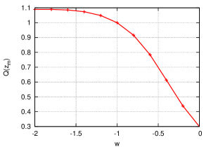
Figure 1: $Q(z_{\rm m})$ as a function of $w$. $D_{\rm A}$ and $\mu$ are given by those in homogeneous and isotropic universe models with $\Omega_{\rm M0}=0.3$ and $\Omega_{\rm X0}=0.7$.

This result shows that there is no regular solution for the inverse problem with $D_{\rm A}$ and $\mu$ for a homogeneous universe model with a dark energy component with $w\neq 1$ in the whole redshift domain. In other words, the existence of the regular solution for the inverse problem cannot be guaranteed for general input functions $D_{\rm A}(z)$ and $\mu(z)$ without the condition (64) as pointed out in Ref. Mustapha:1998jb.

5 Numerical results

5.1 Numerical integration

In this subsection, we consider the distance-redshift relation $D_{\rm A}$ and the redshift-space mass density $\mu$ for a homogeneous and isotropic universe with $(\Omega_{\rm M0},\Omega_{\rm X0})=(0.3,0.7)$, where $\Omega_{\rm X0}$ is the density parameter for the dark energy component whose equation of state is given by $p=w\rho$. The distance-redshift relation satisfies the following second-order differential equation and boundary conditions[18, 19]:

$$\frac{d^{2}D_{\rm A}}{dz^{2}}=-\left(\frac{2}{1+z}+\frac{dH/dz}{H}\right)\frac{dD_{\rm A}}{dz}-\frac{(1+z)D_{\rm A}}{2H^{2}}\left(3\Omega_{\rm M0}+(1+w)\Omega_{\rm X0}(1+z)^{w-2}\right),$$ (74)

$$D_{\rm A}(0)=0~{}~{}~{}{\rm,}~{}~{}~{}\left.\frac{dD_{\rm A}}{dz}\right|_{z=0}=1,$$ (75)

where

$$H=\sqrt{(1+z)^{3}\Omega_{\rm M0}+(1+z)^{w+1}\Omega_{\rm X0}}.$$ (76)

The redshift-space mass density is given by the same expression as Eq. (67).

We numerically integrated Eqs. (34)–(37). Equation (73) is used instead of Eq. (34) for the case $w=-1$. Near the center, solutions can be given in forms of the Maclaurin series, as shown in Appendix B. We use these expressions near the center instead of solving the differential equations. As shown in Fig. 2, we can find a regular solution in the whole redshift domain only for $w=-1$.

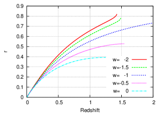
Figure 2: Radial coordinate along the past directed null geodesic as a function of redshift for each value of $w$.

For $w=-1$, $r(z)$, $m(z)$, $k(z)$ and $t_{\rm B}(z)$ are depicted in Fig. 3. $m$, $k$ and $t_{\rm B}$ are depicted as functions of $r$ in Fig. 4. The energy density $\rho$ on the $t=t_{0}$ time slice is depicted as a function of circumferential radius $R(t_{0},r)$ in Fig. 5. This hump type profile has already been found in Ref. Celerier:2009sv and consistent results can be seen in Refs. Kolb:2009hn and Dunsby:2010ts. Our result for $w=-1$ is also consistent with the result in these previous papers.

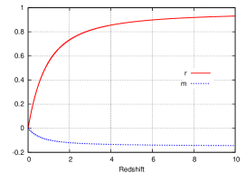
Figure 3: $r$, $k$, $m$ and $t_{\rm B}$ as functions of $z$.

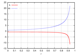
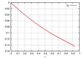
Figure 4: $k$, $m$ and $t_{\rm B}$ as functions of $r$.

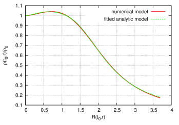
Figure 5: $\rho(t_{0},r)$ as a function of $R(t_{0},r)$ for the numerically obtained model and the model with analytic fitting functions.

5.2 Gauge transformation and fitting functions

We propose fitting functions for the given solution. Before that, for convenience, we perform a gauge transformation $\widetilde{r}=\widetilde{r}(r)$. Hereafter, the “$\widetilde{~}{}$” represents the quantities in the new gauge. We consider the new gauge defined by

$$M(r)=\widetilde{M}(\widetilde{r})=\frac{4\pi}{3}\widetilde{r}^{3}\rho_{0}.$$ (77)

Then, the relation between $r$ and $\widetilde{r}$ is given by

$$\widetilde{r}^{3}=\frac{m(r)}{m_{0}}r^{3}.$$ (78)

The curvature function $\widetilde{k}(\widetilde{r})$ and the big-bang time $\widetilde{t}_{\rm B}(\widetilde{r})$ are given by

$$\widetilde{k}(\widetilde{r})\widetilde{r}^{2}=k(r)r^{2},$$ (79)

$$\widetilde{t}_{\rm B}(\widetilde{r})=t_{\rm B}(r).$$ (80)

We propose analytic fitting functions for $\widetilde{k}$ and $\widetilde{t}_{\rm B}$ as

$$\widetilde{k}_{\rm fit}(\widetilde{r}) = -\frac{7}{10}+0.728893\widetilde{r}-0.634917\widetilde{r}^{2}+0.303959\widetilde{r}^{3}-0.073768\widetilde{r}^{4}-\frac{0.00878216\widetilde{r}}{\widetilde{r}+0.303959},~{}~{}$$ (81)

$$\widetilde{t}_{\rm Bfit}(\widetilde{r}) = -0.21319\widetilde{r}-0.013605\widetilde{r}^{2}+0.000925931\widetilde{r}^{3}+\frac{0.298252\widetilde{r}^{2}}{\widetilde{r}+1.5439}.$$ (82)

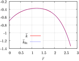
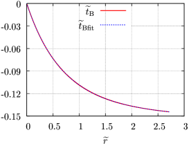
Figure 6: $\widetilde{k}(\widetilde{r})$, $\widetilde{k}_{\rm fit}(\widetilde{r})$, $\widetilde{t}_{\rm B}(\widetilde{r})$ and $\widetilde{t}_{\rm Bfit}(\widetilde{r})$.

The differences in the angular diameter distance and redshift-space mass density between the $\Lambda$CDM model and LTB model with $\widetilde{k}(\widetilde{r})=\widetilde{k}_{\rm fit}(\widetilde{r})$ and $\widetilde{t}_{\rm B}(\widetilde{r})=\widetilde{t}_{\rm Bfit}(\widetilde{r})$ are less than 1%, as shown in Fig. 7.

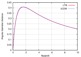
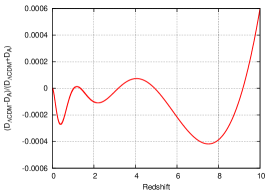
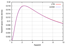
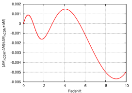
Figure 7: Differences in the angular diameter distance and redshift-space mass density between the $\Lambda$CDM model and LTB model with $\widetilde{k}(\widetilde{r})=\widetilde{k}_{\rm fit}(\widetilde{r})$ and $\widetilde{t}_{\rm B}(\widetilde{r})=\widetilde{t}_{\rm Bfit}(\widetilde{r})$.

2/15

6 Summary

As part of the summary, we describe a theorem and two corollaries based on the analysis in the previous sections after giving three definitions for convenience.

Definition 1

We say that $D_{\rm A}(z)$ is reasonable as a function for the distance-redshift relation if it satisfies the following:

• $D_{\rm A}(z)$ is a $C^{1}$ function on $z>0$ and $\frac{dD_{\rm A}}{dz}$ is piecewise smooth on $z>0$.

• $D_{\rm A}(z)>0$ for $z>0$ and $D_{\rm A}(0)=0$.

• $\left.\frac{dD_{\rm A}}{dz}\right|_{z=0}=1/H_{0}=1$.

• $\frac{dD_{\rm A}}{dz}=0$ at $z=z_{\rm m}$.

• $D_{\rm A}(z)$ is $C^{2}$ and $\frac{d^{2}D_{\rm A}}{dz^{2}}<0$ at $z=z_{\rm m}$

• $\frac{dD_{\rm A}}{dz}\neq 0$ for $z\neq z_{\rm m}$.

Definition 2

We say that $\mu(z)$ is reasonable as a function for the redshift-space mass density if it satisfies the following:

• $\mu(z)$ is finite and positive definite.

• $\mu(z)$ is a piecewise smooth function on $z>0$.

Definition 3

We say that an LTB universe model is observationally regular if the LTB universe model is regular on the past light-cone of the observer at the center except for the big-bang initial singularity.

Theorem

For a set of a reasonable angular diameter distance $D_{\rm A}(z)$ and a reasonable redshift-space mass density $\mu(z)$, there exists the observationally regular LTB universe model whose distance-redshift relation and redshift-space mass density for the observer at the center agree with $D_{\rm A}(z)$ and $\mu(z)$, respectively, if and only if $D_{\rm A}(z)$ and $\mu(z)$ satisfy

$$4\pi\int^{z_{\rm m}}_{0}(1+z)\mu(z)D_{\rm A}(z)dz=1.$$ (83)

Proof

Since

$$B+F=\frac{1}{1+z}\left(1-4\pi\int^{z}_{0}(1+z)\mu(z)D_{\rm A}(z)dz\right),$$

Eq. (83) is equivalent to $B+F=0$. We can find that $(1+z)(B+F)$ is a monotonically decreasing function of $z$, and $B+F$ can vanish only once in $z>0$. If $B+F\neq 0$ at $z=z_{\rm m}$, since $\left.dD_{\rm A}/dz\right|_{z=z_{\rm m}}=0$, we have $\left.dr/dz\right|_{z=z_{\rm m}}=0$ from Eq. (34). Then, from Eq. (18), we find that $\rho$ must be infinite at $z=z_{\rm m}$ for a finite value of $\mu(z_{\rm m})$. Therefore, $B+F$ must vanish at $z=z_{\rm m}$ for the existence of the regular solution. That is, Eq. (83) is a necessary condition for the existence of the regular solution. If the condition (83) is satisfied, from L’Hôpital’s rule, we have

$$\left.\frac{dr}{dz}\right|_{\rm z=z_{\rm m}}=-\left.\frac{d^{2}D_{\rm A}/dz^{2}}{4\pi\mu(z)D_{\rm A}(z)}\right|_{\rm z=z_{\rm m}}>0.$$ (84)

Then, we can find an observationally regular LTB solution solving Eqs. (34)–(37). Q.E.D.

Corollary-1

For an observationally regular LTB universe model in which $\mu(z)$ and $D_{\rm A}(z)$ are reasonable, the distance-redshift relation $D_{\rm A}(z)$ and $\mu(z)$ satisfy $4\pi\int^{z_{\rm m}}_{0}(1+z)\mu(z)D_{\rm A}(z)dz=1$.

Proof

Since Eqs. (34)–(37) are applicable for any LTB universe model, $4\pi\int^{z_{\rm m}}_{0}(1+z)\mu(z)D_{\rm A}(z)dz=1$ must be satisfied so that an LTB universe model is observationally regular. Q.E.D.

Corollary-2

There exist observationally regular LTB universe models whose distance-redshift relation and redshift-space mass density coincide with those in $\Lambda$CDM models.

Proof

As shown in the text, $D_{\Lambda{\rm CDM}}(z)$ and $\mu_{\Lambda{\rm CDM}}(z)$ satisfy the condition (83). Then, this corollary is an immediate consequence from the above theorem. Q.E.D.

The condition (83) has been derived in Ref. Mustapha:1998jb at the first time. Without this condition, we cannot obtain the LTB universe model beyond $z=z_{\rm m}$. We demonstrated this using $D_{\rm A}(z)$ and $\mu(z)$ for flat homogeneous and isotropic universe models with the dark energy component whose equation of state is given by $p=w\rho$. If $w\neq-1$, we cannot obtain the regular LTB solution beyond $z=z_{\rm m}$ by solving the differential equations (34)–(37).

In §5, we have obtained the LTB universe model that realizes the distance-redshift relation and the redshift-space mass density in the $\Lambda$CDM model with $(\Omega_{\rm M0},\Omega_{\rm\Lambda 0})=(0.3,0.7)$. Then, we introduced analytic fitting functions for this numerically obtained LTB model. The LTB model with these analytic fitting functions realize the distance-redshift relation and the redshift-space mass density in the $\Lambda$CDM model within 1% accuracy.

Appendix A Derivation of Eq. (62)

Before the derivation, we provide some useful equations.

• From the expression for $B+F$, we can find

  $$B+F=-\partial_{t}R+\partial_{r}R.$$ (85)

• Differentiating Eq. (3) with $t$, we have

  $$\partial_{t}^{2}R=-\frac{mr^{3}}{6R^{2}}.$$ (86)

• Differentiating Eq. (14) with $z$ along the light-cone, we have

  $$\frac{d}{dz}\partial_{r}R=\frac{d}{dz}\sqrt{1-kr^{2}}~{}~{}\Leftrightarrow~{}~{}\partial_{r}^{2}R=\partial_{t}\partial_{r}R+\partial_{r}\sqrt{1-kr^{2}},$$ (87)

  where we have used the relation

  $$\frac{d}{dz}=\frac{dr}{dz}\partial_{r}+\frac{dt}{dz}\partial_{t}=\frac{dr}{dz}\left(\partial_{r}-\partial_{t}\right).$$ (88)

• Differentiating Eq. (3) with $r$ and dividing both sides by $\sqrt{1-kr^{2}}$, we have

  $$\partial_{r}\sqrt{1-kr^{2}}-\frac{mr^{3}}{6R^{2}}=\frac{\partial_{t}\partial_{r}R\partial_{t}R}{\sqrt{1-kr^{2}}}-\frac{\partial_{r}\left(mr^{3}\right)}{6R\sqrt{1-kr^{2}}}.$$ (89)

First, differentiating Eq. (85) with the redshift $z$, we have

$$\frac{d}{dz}(B+F)=\frac{dr}{dz}\left(\partial_{r}^{2}R+\partial_{t}^{2}R-2\partial_{t}\partial_{r}R\right).$$ (90)

Using Eqs. (86) and (87), we can rewrite the above equation as

$$\frac{d}{dz}(B+F)=\frac{dr}{dz}\left(\partial_{r}\sqrt{1-kr^{2}}-\frac{mr^{3}}{6R^{2}}-\partial_{t}\partial_{r}R\right).$$ (91)

Then, using Eqs. (89) and (14), we have

$$\frac{d}{dz}(B+F) = \frac{dr}{dz}\left(\frac{\partial_{t}\partial_{r}R}{\sqrt{1-kr^{2}}}\left(\partial_{t}R-\partial_{r}R\right)-\frac{\partial_{r}(mr^{3})}{6R\sqrt{1-kr^{2}}}\right)$$ (92)

$$= \frac{dr}{dz}\left(-\frac{\partial_{t}\partial_{r}R}{\sqrt{1-kr^{2}}}\left(B+F\right)-\frac{\partial_{r}(mr^{3})}{6R\sqrt{1-kr^{2}}}\right).$$

Using Eqs. (13), (18) and (34), we can find

$$\frac{d}{dz}(B+F)=-\frac{B+F}{1+z}-4\pi\mu D_{\rm A}$$ (93)

$$\Leftrightarrow \frac{d}{dz}\left((1+z)(B+F)\right)=-4\pi(1+z)\mu D_{\rm A}.$$

Since $\left.(B+F)\right|_{z=0}=1$, we have

$$B+F=\frac{1}{1+z}\left(1-4\pi\int^{z}_{0}(1+z)\mu D_{\rm A}dz\right).$$ (94)

Appendix B Series Expansion of the Solution

We consider the distance-redshift relation $D_{\rm A}$ and the redshift-space mass density $\mu$ for homogeneous and isotropic universes with $(\Omega_{\rm M0},\Omega_{\rm X0},\Omega_{\rm K0}=1-\Omega_{\rm M0}-\Omega_{\rm X0})$ as input functions for the inverse problem given by a set of equations, Eqs. (34) - (37). For the solution near the center, we write functions $r(z)$, $m(z)$, $k(z)$ and $t_{\rm B}(z)$ in the Maclaurin series as follows:

$$r = r_{1}z+\frac{1}{2}r_{2}z^{2}+\frac{1}{6}r_{3}z^{3}+\frac{1}{24}r_{4}z^{4}+\mathcal{O}(z^{5}),$$ (95)

$$m = m_{0}+m_{1}z+\frac{1}{2}m_{2}z^{2}+\frac{1}{6}m_{3}z^{3}+\mathcal{O}(z^{4}),$$ (96)

$$k = k_{0}+k_{1}z+\frac{1}{2}k_{2}z^{2}+\frac{1}{6}k_{3}z^{3}+\mathcal{O}(z^{4}),$$ (97)

$$t_{\rm B} = t_{\rm B1}z+\frac{1}{2}t_{\rm B2}z^{2}+\frac{1}{6}t_{\rm B3}z^{3}+\mathcal{O}(z^{4}).$$ (98)

Substituting these expressions into Eqs. (34)–(37), we can find the values of each coefficient as shown below. For notational simplicity, we use $y:=3w+1$.

$$r(z) = z+\frac{1}{4}(-\Omega_{\rm M0}-\Omega_{\rm X0}y-4)z^{2}$$ (99)

$$+ \frac{1}{24}\left(3\Omega_{\rm M0}^{2}+(6\Omega_{\rm X0}y+8)\Omega_{\rm M0}+\Omega_{\rm X0}(y((3\Omega_{\rm X0}-2)y+8)-4)+24\right)z^{3}$$

$$+ \frac{1}{192}\bigl{(}-15\Omega_{\rm M0}^{3}-9(5\Omega_{\rm X0}y+4)\Omega_{\rm M0}^{2}-3(\Omega_{\rm X0}(y(3(5\Omega_{\rm X0}-2)y+26)-8)+24)\Omega_{\rm M0}$$

$$+ \Omega_{\rm X0}\left(y\left((3(6-5\Omega_{\rm X0})\Omega_{\rm X0}-4)y^{2}-42\Omega_{\rm X0}y+28y+24\Omega_{\rm X0}-92\right)+56\right)-192\bigr{)}z^{4}$$

$$+ O\left(z^{5}\right),$$

$$m(z) = 3\Omega_{\rm M0}+\frac{9\Omega_{\rm M0}z}{2}+\frac{3}{80}\Omega_{\rm M0}(-50\Omega_{\rm M0}+24\Omega_{\rm X0}+10\Omega_{\rm X0}y+60)z^{2}$$ (100)

$$+ \frac{3}{80}\Omega_{\rm M0}\bigl{(}25\Omega_{\rm M0}^{2}-12\Omega_{\rm X0}\Omega_{\rm M0}+20\Omega_{\rm X0}y\Omega_{\rm M0}-50\Omega_{\rm M0}-5\Omega_{\rm X0}^{2}y^{2}+5\Omega_{\rm X0}y^{2}+22\Omega_{\rm X0}$$

$$- 12\Omega_{\rm X0}^{2}y+20\Omega_{\rm X0}y+10\bigr{)}z^{3}+O\left(z^{4}\right),$$

$$k(z) = -1+\Omega_{\rm M0}+\left(\Omega_{\rm M0}-\frac{\Omega_{\rm X0}y}{2}-1\right)z$$ (101)

$$+ \frac{1}{240}\left(-100\Omega_{\rm M0}^{2}+2(\Omega_{\rm X0}(25y+36)+80)\Omega_{\rm M0}-5\Omega_{\rm X0}(y((8-3\Omega_{\rm X0})y+16)+16)-60\right)z^{2}$$

$$+ \frac{1}{480}\bigl{(}100\Omega_{\rm M0}^{3}+(\Omega_{\rm X0}(50y-72)-200)\Omega_{\rm M0}^{2}$$

$$+ (\Omega_{\rm X0}(y(50y-\Omega_{\rm X0}(65y+72)+190)+148)+100)\Omega_{\rm M0}$$

$$- 5\Omega_{\rm X0}(y(y((3(\Omega_{\rm X0}-2)\Omega_{\rm X0}+4)y+4)+24)+8)\bigr{)}z^{3}+O\left(z^{4}\right),$$

$$t_{\rm B}(z) = -\frac{(\Omega_{\rm X0}(3t_{0}-2)y)z}{4(\Omega_{\rm M0}-1)}$$ (102)

$$+ \frac{\Omega_{\rm X0}}{1920(\Omega_{\rm M0}-1)^{3}}\Bigl{(}-8(-36\Omega_{\rm M0}t_{0}+48t_{0}-8)(\Omega_{\rm M0}-1)^{2}$$

$$- 10(24\Omega_{\rm X0}\Omega_{\rm M0}-18\Omega_{\rm X0}t_{0}\Omega_{\rm M0}+48t_{0}\Omega_{\rm M0}-32\Omega_{\rm M0}-84\Omega_{\rm X0}$$

$$+ 108\Omega_{\rm X0}t_{0}-48t_{0}+32)y^{2}(\Omega_{\rm M0}-1)$$

$$+ 4\left(90t_{0}\Omega_{\rm M0}^{2}-60\Omega_{\rm M0}^{2}+90t_{0}\Omega_{\rm M0}-60\Omega_{\rm M0}-180t_{0}+120\right)y(\Omega_{\rm M0}-1)\Bigr{)}z^{2}$$

$$+ \frac{\Omega_{\rm X0}}{1920(\Omega_{\rm M0}-1)^{3}}\Bigl{(}-5\bigl{(}2(12t_{0}+\Omega_{\rm X0}(-18t_{0}+3\Omega_{\rm X0}(3t_{0}-4)+20)-8)\Omega_{\rm M0}^{2}$$

$$+ \left((92-81t_{0})\Omega_{\rm X0}^{2}+32(6t_{0}-5)\Omega_{\rm X0}-48t_{0}+32\right)\Omega_{\rm M0}$$

$$+ 2(12t_{0}+3\Omega_{\rm X0}(-26t_{0}+\Omega_{\rm X0}(28t_{0}-23)+20)-8)\bigr{)}y^{3}$$

$$- 10(\Omega_{\rm M0}-1)(-24\Omega_{\rm X0}\Omega_{\rm M0}^{2}+27\Omega_{\rm X0}t_{0}\Omega_{\rm M0}^{2}-18t_{0}\Omega_{\rm M0}^{2}+12\Omega_{\rm M0}^{2}+30\Omega_{\rm X0}\Omega_{\rm M0}$$

$$- 54\Omega_{\rm X0}t_{0}\Omega_{\rm M0}-30t_{0}\Omega_{\rm M0}+20\Omega_{\rm M0}+84\Omega_{\rm X0}-108\Omega_{\rm X0}t_{0}+48t_{0}-32)y^{2}$$

$$+ 4(\Omega_{\rm M0}-1)(-45t_{0}\Omega_{\rm M0}^{3}+30\Omega_{\rm M0}^{3}-36\Omega_{\rm X0}t_{0}\Omega_{\rm M0}^{2}+120t_{0}\Omega_{\rm M0}^{2}-40\Omega_{\rm M0}^{2}-40\Omega_{\rm X0}\Omega_{\rm M0}$$

$$+ 126\Omega_{\rm X0}t_{0}\Omega_{\rm M0}-255t_{0}\Omega_{\rm M0}+90\Omega_{\rm M0}+60\Omega_{\rm X0}-120\Omega_{\rm X0}t_{0}+180t_{0}-80)y$$

$$- 8(\Omega_{\rm M0}-1)^{2}\left(18t_{0}\Omega_{\rm M0}^{2}-9t_{0}\Omega_{\rm M0}+18\Omega_{\rm M0}-48t_{0}+8\right)\Bigr{)}z^{3}+O\left(z^{4}\right).$$

Appendix C Inverse Problem with $t_{\rm B}(r)=0$

Here, we show how to solve the inverse problem using the INN approach with $t_{\rm B}(r)=0$ for a given angular diameter distance $D_{\rm A}(z)$. This has been carried out in Ref. Yoo:2008su by solving a set of four differential equations parametrized by an affine parameter on the null geodesic. Here, we do not use the affine parameter but the redshift $z$ as the independent variable. In this procedure, the number of differential equations is reduced to three.

C.1 Basic equations

Basic equations are derived by replacing the condition (18) with $t_{\rm B}(z)=0$. Then, we have the following three coupled first-order differential equations:

$$\frac{dr}{dz} = \frac{1}{B+F}\frac{dD_{\rm A}}{dz},$$ (103)

$$\frac{dm}{dz} = \frac{1}{DG-CH}\left(\frac{\sqrt{1-kr^{2}}}{1+z}D-(HF+DJ)\frac{dr}{dz}\right),$$ (104)

$$\frac{dk}{dz} = \frac{1}{D}\left(F\frac{dr}{dz}-C\frac{dm}{dz}\right).$$ (105)

C.2 Solutions near the center

We perform the Maclaurin series expansion as (39)–(52). Substituting these expressions into Eqs. (103)–(105), we find

$$r(z) = z+\frac{1}{2}(D_{\rm A2}+1)z^{2}+\frac{1}{12}(4D_{\rm A2}+2D_{\rm A3}+m_{0})z^{3}+O\left(z^{4}\right),$$ (106)

$$m(z) = m_{0}+\frac{m_{0}(m_{0}+D_{\rm A2}(6-9t_{0})-18t_{0}+9)z}{(m_{0}+6)t_{0}-6}+O\left(z^{2}\right),$$ (107)

$$k(z) = \frac{m_{0}-3}{3}+\frac{(m_{0}-3)(m_{0}-6D_{\rm A2}(t_{0}-1)-12t_{0}+12)z}{3((m_{0}+6)t_{0}-6)}+O\left(z^{2}\right).$$ (108)

Then, we find that the parameter $m_{0}$ can be freely chosen differently from the MHE approach. We use this degree of freedom to guarantee $B+F=0$ at $z=z_{\rm m}$.

C.3 Numerical procedure to solve the differential equations

For illustrative purposes, we rewrite Eqs. (103)–(105) in abstract forms as

$$\frac{dr}{dz} = \frac{1}{X(z,r,m,k)}\frac{dD_{\rm A}}{dz},$$ (109)

$$\frac{dm}{dz} = Y\left(z,r,m,k,\frac{dr}{dz}\right),$$ (110)

$$\frac{dk}{dz} = Z\left(z,r,m,k,\frac{dr}{dz},\frac{dm}{dz}\right).$$ (111)

Then, the procedure to solve Eqs.(103)-(105) is summarized in follows:

1. We determine a trial value for $m_{0}$.

2. We solve the differential equations from the center, where, near the center, we use the expressions (106)–(108) instead of solving the differential equations.

3. We stop integrating the equations at $z=z_{\rm b}<z_{\rm m}$ and read off the values of $r$, $m$ and $k$ at this point. We label these values as $r_{\rm b-}$, $m_{\rm b-}$ and $k_{\rm b-}$.

4. We determine trial values for $m_{\rm m}$ and $k_{\rm m}$, where the subscript “m” denotes the value at $z=z_{\rm m}$.

5. We numerically solve the equation $X(z_{\rm m},r_{\rm m},m_{\rm m},k_{\rm m})=0$ for $r_{\rm m}$.

6. At $z=z_{\rm m}$, Eq. (109) can be rewritten as

   $$\left.\frac{dr}{dz}\right|_{z=z_{\rm m}}=\left.\frac{\frac{d^{2}D_{\rm A}}{dz^{2}}}{\frac{dX}{dz}(z,r,m,k,dr/dz,dm/dz,dk/dz)}\right|_{z=z_{\rm m}}.$$ (112)

   Then, Eqs. (110)–(112) can be regarded as simultaneous equations for $dr/dz|_{z=z_{\rm m}}$, $dm/dz|_{z=z_{\rm m}}$ and $dk/dz|_{z=z_{\rm m}}$. We numerically solve them.

7. We integrate the differential equations (103)–(105) from $z=z_{\rm m}$ backward.

8. We stop integrating the equations at $z=z_{\rm b}$ and read off the values of $r$, $m$ and $k$ at this point. We label these values as $r_{\rm b+}$, $m_{\rm b+}$ and $k_{\rm b+}$.

9. We define deviations $\delta r$, $\delta m$ and $\delta k$ as follows:

   $$\delta r := r_{\rm b-}-r_{\rm b+},$$ (113)

   $$\delta m := m_{\rm b-}-m_{\rm b+},$$ (114)

   $$\delta k := k_{\rm b-}-k_{\rm b+}.$$ (115)

10. Operations 1–9 give the deviations $\delta r$, $\delta m$ and $\delta k$ for given values of $m_{0}$, $m_{\rm m}$ and $k_{\rm m}$. That is, we can define $\delta r=\delta r(m_{0},m_{\rm m},k_{\rm m})$, $\delta m=\delta m(m_{0},m_{\rm m},k_{\rm m})$ and $\delta k=\delta k(m_{0},m_{\rm m},k_{\rm m})$ as functions of $m_{0}$, $m_{\rm m}$ and $k_{\rm m}$ using operations 1–9. Then, repeating operations 1–9 and using the Newton-Raphson method, we numerically solve the equations

    $$\delta r(m_{0},m_{\rm m},k_{\rm m}) = 0,$$ (116)

    $$\delta m(m_{0},m_{\rm m},k_{\rm m}) = 0,$$ (117)

    $$\delta k(m_{0},m_{\rm m},k_{\rm m}) = 0$$ (118)

    for $m_{0}$, $m_{\rm m}$ and $k_{\rm m}$. Eventually, we have functional forms of $r(z)$, $m(z)$ and $k(z)$ in $z<z_{\rm m}$ without discontinuity at $z=z_{\rm b}$.

11. Finally, we solve the differential equations (103)–(105) from $z=z_{\rm m}$ forward with initial conditions $r(z_{\rm m})=r_{\rm m}$, $m(z_{\rm m})=m_{\rm m}$ and $k(z_{\rm m})=k_{\rm m}$ given above.

C.4 Results

We performed operations 1–11 in the previous subsection using the distance-redshift relation in the $\Lambda$CDM model with $(\Omega_{\rm M0},\Omega_{\Lambda 0})=(0.3,0.7)$. The result is consistent with that in Ref. Yoo:2008su. We performed the same gauge transformation as that given in §5. Then, we find a fitting function for $\tilde{k}(\tilde{r})$ as[20]

$$\tilde{k}_{\rm fit}(\tilde{r})=\frac{0.545745}{0.211472+\sqrt{0.026176+\tilde{r}}}-\frac{2.22881}{\left(0.807782+\sqrt{0.026176+\tilde{r}}\right)^{2}}.$$ (119)

The angular diameter distance in the LTB universe model with $\tilde{k}(\tilde{r})=\tilde{k}_{\rm fit}(\tilde{r})$ is depicted in the Fig. 8. The deviation of the distance from that in the $\Lambda$CDM model is within 0.1%.

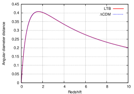
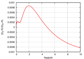
Figure 8: Distance-redshift relations in the $\Lambda$CDM model with $(\Omega_{\rm M0},\Omega_{\Lambda 0})=(0.3,0.7)$ and the LTB model with $(\tilde{t}_{\rm B}(\tilde{r}),\tilde{k}(\tilde{r}))=(0,\tilde{k}_{\rm fit}(\tilde{r}))$(left panel) and the deviation of the distance(right panel).

References

- [1] G. Lemaître, Gen. Relat. Gravit. 29 (1997), 641.
- [2] R. C. Tolman, Proc. Natl. Acad. Sci. 20, 169 (1934).
- [3] H. Bondi, Mon. Not. R. Astron. Soc. 107, 410 (1947).
- [4] N. Mustapha, C. Hellaby and G. F. R. Ellis, Mon. Not. R. Astron. Soc. 292, 817 (1997), arXiv:gr-qc/9808079.
- [5] T. H.-C. Lu and C. Hellaby, Class. Quantum Grav. 24, 4107 (2007), arXiv:0705.1060.
- [6] M. L. McClure and C. Hellaby, Phys. Rev. D78, 044005 (2008), arXiv:0709.0875.
- [7] M.-N. Célérier, K. Bolejko and A. Krasinski, Astron. Astrophys. 518, A21 (2010), arXiv:0906.0905.
- [8] E. W. Kolb and C. R. Lamb, arXiv:0911.3852.
- [9] P. Dunsby, N. Goheer, B. Osano and J.-P. Uzan, arXiv:1002.2397.
- [10] C.-M. Yoo, T. Kai, and K. Nakao, Prog. Theor. Phys. 120, 937 (2008), arXiv:0807.0932.
- [11] M.-N. Célérier, Astron. Astrophys. 353, 63 (2000), arXiv:astro-ph/9907206.
- [12] D. J. H. Chung and A. E. Romano, Phys. Rev. D74, 103507 (2006), arXiv:astro-ph/0608403.
- [13] R. A. Vanderveld, E. E. Flanagan and I. Wasserman, Phys. Rev. D74, 023506 (2006), arXiv:astro-ph/0602476.
- [14] A. E. Romano, arXiv:0912.4108.
- [15] A. E. Romano, arXiv:0912.2866.
- [16] C. Hellaby, Mon. Not. R. Astron. Soc. 370, 239 (2006), arXiv:astro-ph/0603637.
- [17] M. Tanimoto and Y. Nambu, Class. Quantum Grav. 24, 3843 (2007), arXiv:gr-qc/0703012.
- [18] E. V. Linder, Astron. Astrophys. 206, 190 (1988).
- [19] M. Sereno, G. Covone, E. Piedipalumbo and R. de Ritis, Mon. Not. R. Astron. Soc. 327, 517 (2001), arXiv:astro-ph/0102486.
- [20] C.-M. Yoo, K. Nakao and M. Sasaki, JCAP 1007, 012 (2010).