Three-dimensional rogue waves in non-stationary parabolic potentials

Abstract

Using symmetry analysis we systematically present a higher-dimensional similarity transformation reducing the (3+1)-dimensional inhomogeneous nonlinear Schrödinger (NLS) equation with variable coefficients and parabolic potential to the (1+1)-dimensional NLS equation with constant coefficients. This transformation allows us to relate certain class of localized exact solutions of the (3+1)-dimensional case to the variety of solutions of integrable NLS equation of (1+1)-dimensional case. As an example, we illustrated our technique using two lowest order rational solutions of the NLS equation as seeding functions to obtain rogue wave-like solutions localized in three dimensions that have complicated evolution in time including interactions between two time-dependent rogue wave solutions. The obtained three-dimensional rogue wave-like solutions may raise the possibility of relative experiments and potential applications in nonlinear optics and BECs.

I Introduction

Similarity analysis is one of modern powerful techniques which allows us to find self-similar solutions of equations that previously were known to be non-integrable (see, e.g., BK and references therein). They do not provide the complete integrability. However, they help to produce selected solutions in analytical form which may be important for variety of applications. One of the representative examples is the nonlinear Schrödinger (NLS) equation. It is well known that in (1+1)-dimension ((1+1)-D) this equation is completely integrable by inverse scattering technique IST . In (2+1)-D the equation is not integrable. However, solutions localized in two transverse directions do exist Chiao64 but may be unstable and subjected to collapse Vlasov ; Berge . They are mostly known from numerical simulations Akhmanov . Remarkably, some of the localized solutions can be found using similarity reductions Gagnon . Despite being unphysical, exact solutions provide some insight on the properties of the equation that is important for many applications. Clearly, adding a dimension changes drastically integrability properties of the equation. Thus, (3+1)-D NLS equation is not an exception and we are faced with the problem of finding its solutions knowing that they are not directly related to the solutions of the same equation in lower dimensionality.

The NLS equation in (3+1)-D is an important model for variety of physical problems Optics ; BEC . It is used in nonlinear optics Optics , condensed matter physics and in particular in modelling Bose-Einstein condensate (BEC) BEC . Numerical solutions can be found with various techniques but the value of an analytical approach is significant by itself. In this work, extending the ideas of  yanvk ; YH we use the similarity transformations to reduce the dimensionality of the equation from (3+1)-D to (1+1)-D. In the former case, the coefficients in the equation are variable while in the latter they can be chosen to be constants. This allows us to use the complete integrability of the (1+1)-D equation.

More specifically, we will focus on the possibility of constructing truly three-dimensional rogue waves, i.e. waves whose dynamics essentially depends on all spatial coordinates, although it is possible to identify the coordinate in which the motion is effectively one-dimensional. This example is directly related to the description of matter wave dynamics in the mean-field approximation (where the NLS equation is also known as the Gross-Pitaevskii equation), thus representing a unique possibility of creating and observing three-dimensional rogue matter waves. We note that the conventional rogue waves are either two-dimensional, as it happens, e.g., in the ocean ocean , in wide aperture optical cavities Arecchi and in capillary wave experiments Shats or one-dimensional and they appear in many fields including nonlinear optics Solli-Eggleton ; Yeom ; BKA-opt ; ypla10 , cigar-shaped BECs BKA , atmosphere at , and finances yan09 .

The rest of this paper is organized as follows. In Sec. II, we describe the (1+1)-D similarity transformation reducing the (3+1)-D inhomogeneous nonlinear Schrödinger (NLS) equation with variable coefficients and parabolic potential to the (1+1)-D NLS equation with constant coefficients. In Sec. III, we determine the self-similar variables and constraints satisfied by the coefficients in the (3+1)-D inhomogeneous NLS equation. Moreover, we give some comments about these coefficients. Sec. IV mainly discusses two types of localized 3D rogue wave-like solutions, which profiles are exhibited. Finally, we give some conclusions in Sec. V.

II The 3D model and similarity reductions

The original three-dimensional inhomogeneous NLS equation with variable coefficients can be written in a dimensionless form:

$$i\frac{\partial\Psi}{\partial t}=-\frac{1}{2}\nabla^{2}\Psi+v({\bf r},t)\Psi+g(t)|\Psi|^{2}\Psi+i\gamma(t)\Psi,$$ (1)

where the physical field $\Psi\equiv\Psi({\bf r},t)$, ${\bf r}\in\mathbb{R}^{3}$, $\nabla\equiv(\partial_{x},\partial_{y},\partial_{z})$ with $\partial_{x}\equiv\partial/\partial x$, the external potential $v({\bf r},t)$ is a real-valued function of time and spatial coordinates, the nonlinear coefficient $g(t)$ and gain/loss coefficient $\gamma(t)$ are real-valued functions of time. This equation arises in many fields such as nonlinear optics (see, e.g., Optics ) and BECs (alias the three-dimensional Gross-Pitaevskii equation with variable coefficients, see, e.g.,  BEC ; yanvk ; YH ).

We search for a similar transformation connecting solutions of Eq. (1) with those of the (1+1)-D standard NLS equation with constant coefficients, i.e.

$$\begin{array}[]{l}\displaystyle i\frac{\partial\Phi(\eta,\tau)}{\partial\tau}=-\frac{\partial^{2}\Phi(\eta,\tau)}{\partial\eta^{2}}+G|\Phi(\eta,\tau)|^{2}\Phi(\eta,\tau).\end{array}$$ (3)

Here the physical field $\Phi(\eta,\tau)$ is a function of two variables $\eta\equiv\eta({\bf r},t)$ and $\tau\equiv\tau(t)$ which are to be determined, and $G$ is a constant. Since our main goal is to study three-dimensional rogue waves, we choose $G=-1$ which corresponds to the attractive case (or focusing nonlinearity in optics and negative scattering lengths in the BEC theory). In order to control boundary conditions at infinity we impose the natural constraints yanvk

$$\eta\to 0\quad\mbox{at}\quad{\bf r}\to 0\quad\mbox{and}\quad\eta\to\infty\quad\mbox{at}\quad{\bf r}\to\infty.$$ (4)

We are looking for the physical field $\Psi({\bf r},t)$ in the form of the ansatz  YH

$$\begin{array}[]{l}\Psi({\bf r},t)=\rho(t)e^{i\varphi({\bf r},t)}\Phi[\eta({\bf r},t),\tau(t)]\end{array}$$ (6)

with $\rho(t)$ and $\varphi({\bf r},t)$ (like $\tau(t)$, and $\eta({\bf r},t)$, introduced above) being the real-value functions of the indicated variables, The ansatz (6) allows us to reduce the problem to (1+1)-D one (we notice that it differs from the one-dimensional stationary reductions Juan2 ; yanvk ). Variables in this reduction are to be determined from the requirement for the new function $\Phi(\eta({\bf r},t),\tau(t))$ to satisfy Eq. (3) (we notice that there also exist other similar reductions for Eq. (1) which require that $\Phi(\eta,\tau)$ may satisfy other nonlinear equations). Thus, we substitute the transformation (6) into Eq. (1) and after relatively simple algebra obtain the system of partial differential equations

$$\nabla^{2}\eta=0,\ \ \eta_{t}+\nabla\varphi\cdot\nabla\eta=0,\ \ 2\tau_{t}-|\nabla\eta|^{2}=0,\quad$$ (7a)

$$2\rho_{t}+\rho\nabla^{2}\varphi-2\gamma(t)\rho=0,$$ (7b)

$$2g(t)\rho^{2}-G|\nabla\eta|^{2}=0,$$ (7c)

$$2v({\bf r},t)+|\nabla\varphi|^{2}+2\varphi_{t}=0.$$ (7d)

Generally speaking, equations in the system (7) are not compatible with each other when linear and nonlinear potentials are arbitrary. One, however, can pose the problem to find the functions $v({\bf r},t)$, $g(t)$ and $\gamma(t)$ such that the system (7) becomes solvable. This requirement leads us to the procedure which can be outlined as follows.

• Firstly, we solve Eq. (7a) subject to the boundary conditions (4) thus obtaining the similarity variables $\eta({\bf r},t),\tau(t)$ and the phase $\varphi({\bf r},t)$.

• Secondly, we consider Eqs. (7b)-(7d) as definitions for the functions $\rho(t),\ v({\bf r},t)$ and $g(t)$ in terms of already known functions $\eta({\bf r},t),\tau(t)$ and $\varphi({\bf r},t)$.

Note that the first step determines transformation of variables which does not involve explicitly any specific time dependent coefficients. However, these coefficients may appear after integration of these equations. The second step determines the coefficients which are compatible with the above change of variables. Thus, it leads to the model (3). In this approach, the function $\eta({\bf r},t)$ defines the surface where the wave has a constant amplitude. The function $\varphi({\bf r},t)$ determines the wave-front solution (the manifold of the constant phase).

Thus, we can establish a correspondence between selected solutions of the (3+1)-dimensional inhomogeneous NLS equation with variable coefficients (1) and known solutions of completely integrable NLS equation (3). The latter has an infinite number of solutions thereby giving us a chance to look for physically relevant solutions of the (3+1)-dimensional case. In particular, we can relate them to the recently studied rogue wave solutions of the NLS equation AAS ; AAT ; ASA ; ACA . As a consequence, we obtain three-dimensional time-dependant rogue wave solutions of Eq. (1).

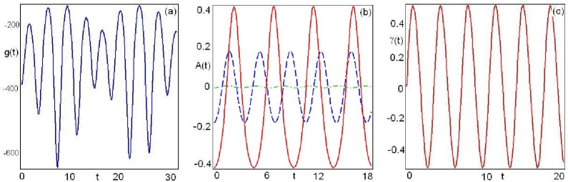
Figure 1: (color online). Profiles of (a) nonlinearity $g(t)$ given by Eq. (9b), (b) the coefficients $A_{x}(t)$ (solid line), $A_{y}(t)$ (dashed line), and $A_{z}(t)$ (dashed-dotted line) of second degree term of the linear potential $v({\bf r},t)$ given by Eq. (10) and (c) the gain/loss term $\gamma(t)$ vs time for the parameters are given by Eq. (20) with $k_{x}=0.9,\,k_{y}=0.6,\ k_{z}=0.1$ and $k=0.6$.

III Variables and coefficients of the transformation

Solving Eq. (7a) we can write the similarity variables $\eta({\bf r},t),\ \tau(t)$ and the phase $\varphi({\bf r},t)$ in the form

$$\eta({\bf r},t)={\bf c}(t)\cdot{\bf r}-\int^{t}_{0}{\bf c}(s)\cdot{\bf a}(s)ds,$$ (8a)

$$\tau(t)=\displaystyle\frac{1}{2}\int^{t}_{0}|{\bf c}(s)|^{2}ds,$$ (8b)

$$\varphi({\bf r},t)={\bf r}\,\hat{\Omega}(t)\,{\bf r}+{\bf a}(t)\cdot{\bf r}+\omega(t)$$ (8c)

where we have introduced the diagonal time-dependent 3$\times$3 matrix $\hat{\Omega}(t)={\rm diag}(\Omega_{x}(t),\Omega_{y}(t),\Omega_{z}(t))$ with $\Omega_{\sigma}(t)=-\dot{c}_{\sigma}(t)/[2c_{\sigma}(t)]$ (hereafter $\sigma=x,y,z$ and an overdot stands for the derivative with respect to time). The coefficients ${\bf c}(t)=(c_{x}(t),c_{y}(t),c_{z}(t))$, ${\bf a}(t)=(a_{x}(t),a_{y}(t),a_{z}(t))$ and $\omega(t)$ are time-dependent functions.

Now, from Eqs. (7b)-(7d) we obtain the functions $\rho(t),\ v({\bf r},t)$ and $g(t)$ in the form

$$\rho(t)=\rho_{0}\sqrt{|c_{x}(t)\,c_{y}(t)\,c_{z}(t)|}\,e^{\int^{t}_{0}\gamma(s)ds},$$ (9a)

$$g(t)=\frac{G\,|{\bf c}(t)|^{2}}{2\rho_{0}^{2}\,|c_{x}(t)\,c_{y}(t)\,c_{z}(t)|\,e^{2\int^{t}_{0}\gamma(s)ds}},$$ (9b)

$$v({\bf r},t)={\bf r}\,\hat{A}(t)\,{\bf r}+{\bf b}(t)\cdot{\bf r}-\dot{\omega}(t)-\frac{1}{2}|{\bf a}(t)|^{2},$$ (9c)

where $\rho_{0}$ is an integration constant.

A few comments would be useful here. First, the gain/loss term $\gamma(t)$, is determined in the initial statement of the problem and can serve as an additional control function or a parameter if it is a constant. Then changing the time-dependent dissipation we can excite different dynamical regimes. Second, the change of the all parameters is interrelated. In practical terms such a time dependence can be performed in different ways for different physical systems. In particular, in the context of the BEC applications, this can be done by simultaneous change of the frequency of the lasers controlling the external trap $v({\bf r},t)$ and the detuning from the Feshbach resonance, responsible for the variation of $g(t)$. Finally, we notice that one can consider the case of $g(t)\equiv$const which however is reduced to the trivial case of a plane wave, whose parameters change along the chosen direction (determined by the vector ${\bf c}$ which is a constant in this case). Such solutions will not be considered here.

In writing the linear potential $v({\bf r},t)$ we have defined the diagonal time-dependent 3$\times$3 matrix $\hat{A}(t)=$diag$(A_{x}(t),A_{y}(t),A_{z}(t))$ with the entries

$$A_{\sigma}(t)=\frac{\ddot{c}_{\sigma}(t)}{2c_{\sigma}(t)}-\frac{\dot{c}_{\sigma}^{2}(t)}{c_{\sigma}^{2}(t)}$$ (10)

and the vector function ${\bf b}(t)=(b_{x}(t),b_{y}(t),b_{z}(t))$ with the entries

$$b_{\sigma}(t)=\frac{\dot{c}_{\sigma}(t)\,a_{\sigma}(t)}{c_{\sigma}(t)}-\dot{a}_{\sigma}(t).$$ (11)

It is easy to see that the velocity field ${\bf v}({\bf r},t)=\nabla\varphi({\bf r},t)$ corresponding to the above-mentioned phase $\varphi({\bf r},t)$ is given by

$$\begin{array}[]{l}{\bf v}({\bf r},t)=2(\Omega_{x}(t)x,\,\Omega_{y}(t)y,\,\Omega_{z}(t)z)+{\bf a}(t)\end{array}$$ (13)

such that we have the divergence of the vector field ${\bf v}({\bf r},t)$ in the form

$$\begin{array}[]{rl}{\rm div}\,{\bf v}({\bf r},t)&=2[\Omega_{x}(t)+\Omega_{y}(t)+\Omega_{z}(t)]\vspace{0.08in}\cr&=-\partial_{t}\ln|c_{x}(t)c_{y}(t)c_{z}(t)|.\end{array}$$ (16)

Thus the zeros of any of the components of ${\bf c}(t)$ means the divergence of the field, which occurs at the instants when the nonlinearity $g(t)$ becomes infinite [see (9b)]. Such cases will not be considered in the present paper.

It follows from Eqs. (9c) and (10) that if we require that the linear potential $v({\bf r},t)$ is a second degree polynomial for every space $x,\ y,\ z$, then we have $A_{\sigma}\not=0$, i.e., $c_{\sigma}\ddot{c}_{\sigma}-2\dot{c}_{\sigma}^{2}\not=0$, which denote that $c_{\sigma}$ are not equivalent to constants but some functions of time. These time-dependent functions $c_{\sigma}(t)$ will affect on the other variables (see Eqs. (8a)-11)) such that self-similar solutions of Eq. (1) in the form (6) exhibit abundant structures. In what follows we will use specific solutions (e.g., rogue wave solutions) of the NLS equation to illustrate the nontrivial dynamics of three-dimensional rogue wave-like solutions defined by the Eq. (1) for the different parameters mentioned above.

IV Two types of localized 3D rogue wave-like solutions

As two representative examples, we consider the lowest order rational solutions of the NLS equation which serve as prototypes of rogue waves. First, we use the first order rational solution of Eq. (3) (see AAS ). As a result, we obtain the first-order non-stationary rogue wave solutions of Eq. (1) in the form

$$\Psi_{1}({\bf r},t)=\rho_{0}\sqrt{|c_{x}(t)\,c_{y}(t)\,c_{z}(t)|}\,e^{\int^{t}_{0}\gamma(s)ds}\qquad\qquad$$

$$\times\left[1-\frac{4+8i\tau(t)}{1+2\eta^{2}({\bf r},t)+4\tau^{2}(t)}\right]e^{i[\varphi({\bf r},t)+\tau(t)]},$$ (17)

where the variables $\eta({\bf r},t),\ \tau(t)$ and the phase $\varphi({\bf r},t)$ are given by Eqs. (8a)-(8c).

For the illustrative purposes, we can choose these free parameters in the form

$$\begin{array}[]{l}c_{\sigma}(t)=a_{\sigma}(t)={\rm dn}(t,k_{\sigma}),\vspace{0.05in}\cr\rho_{0}=1,\,\gamma(t)={\rm sn}(t,k){\rm cn}(t,k),\end{array}$$ (20)

(where dn, sn, and cn stand for the respective Jacobi elliptic functions, and $k_{\sigma},k$ are their moduli.) and $\omega(t)=0$. Figure 1 depicts the profiles of nonlinearity $g(t)$ given by Eq. (9b), the coefficients of second degree terms of the linear potential $v({\bf r},t)$ given by Eq. (10) and the gain/loss term $\gamma(t)$ vs time for the chosen parameters given by Eq. (20). The evolution of intensity distribution of the 3D field (17) is shown in Fig. 2. We can see that the simple Lorenzian function of the (1+1)D case is transformed into a significantly more complicated evolution along the $t$-axis. The solution is localized in space and keeps the localization infinitely in time, which differs from the usual rogue wave solutions (see ASA2).

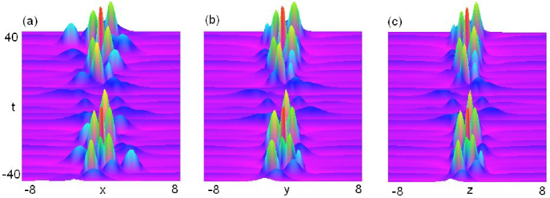
Figure 2: (color online). Color coded plot of wave intensity (a) $|\Psi_{1}|^{2}(x,0,0,t)$ with $\max_{\{x,0,0,t\}}|\Psi_{1}|^{2}=0.06$, (b) $|\Psi_{1}|^{2}(0,y,0,t)$ with $\max_{\{0,y,0,t\}}|\Psi_{1}|^{2}=0.068$ and (c) $|\Psi_{1}|^{2}(0,0,z,t)$ with $\max_{\{0,0,z,t\}}|\Psi_{1}|^{2}=0.068$ defined by the solution (17) for the parameters given by Eq. (20) with $k_{x}=0.9,\,k_{y}=0.6,\,k_{z}=0.1,\ k=0.6$. Note that for given set of parameters, the wave is localized in space.

On the other hand, if we choose the free parameters in the form

$$\begin{array}[]{l}c_{x}(t)=a_{x}(t)=1+c_{0}\sin(t),\cr c_{y}(t)=a_{y}(t)=1.2+c_{0}\cos(t),\cr c_{z}(t)=a_{z}(t)=0.8+c_{0}\sin(t),\ c_{0}=0.01\end{array}$$ (24)

and $\rho_{0},\,\omega(t)$ and $\gamma(t)$ are same as the ones given by Eq. (20), then the evolution of intensity distribution of the 3D rogue wave solutions (17) will be changed. Figure 3 displays the profiles of nonlinearity $g(t)$ given by Eq. (9b) and the coefficients of second degree terms of the linear potential $v({\bf r},t)$ given by Eq. (10) vs time for the chosen parameters given by Eq. (24). For this case, the 3D rogue wave solution (17) is shown in Figs. 4. The solution is localized both in time and in space thus revealing the usual “rogue wave” features. It is worth emphasizing here, that although the “generating” function ${\bf c}(t)$ was chosen as monochromatic function, the respective change of the nonlinearity $g(t)$ required for the existence of the exact solution is periodic but depending on various frequencies. This is natural reflection of the fact that we are dealing with a nonstationary solution of the nonlinear problem, characterized by the generation of multiple frequencies.

Generally speaking, we have large degree of freedom in choosing the coefficients of transformation. As a result, we can describe infinitely large class of solutions of three-dimensional NLS equation with every exact solution of the one-dimensional NLS equation. Additional possibility of choosing the solution of the latter one increases tremendously variety of solutions that we can obtain.

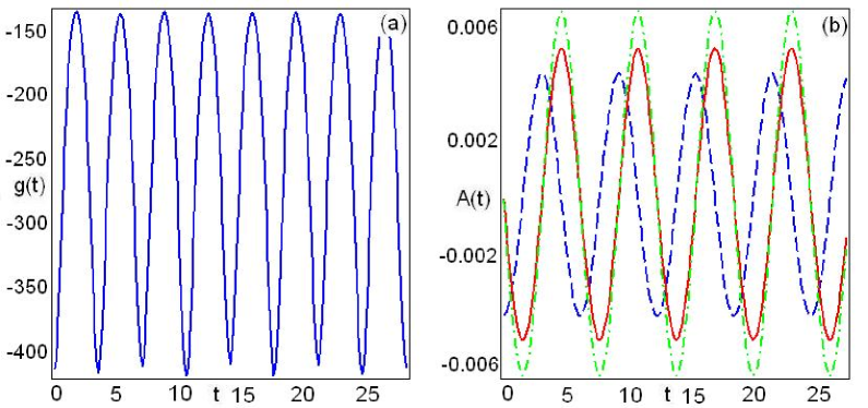
Figure 3: (color online). Profiles of (a) nonlinearity $g(t)$ given by Eq. (9b) and (b) the coefficients $A_{x}(t)$ (solid line), $A_{y}(t)$ (dashed line), and $A_{z}(t)$ (dashed-dotted line) of second degree term of the linear potential $v({\bf r},t)$ given by Eq. (10) vs time for the parameters are given by Eq. (24).

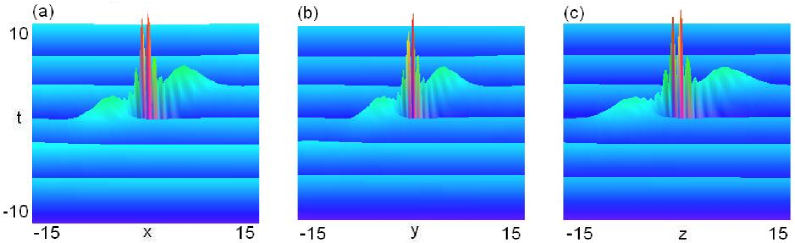
Figure 4: (color online). Color coded plot of wave intensity (a) $|\Psi_{1}|^{2}(x,0,0,t)$ with $\max_{\{x,0,0,t\}}|\Psi_{1}|^{2}=0.027$, (b) $|\Psi_{1}|^{2}(0,y,0,t)$ with $\max_{\{0,y,0,t\}}|\Psi_{1}|^{2}=0.03$ and (c) $|\Psi_{1}|^{2}(0,0,z,t)$ with $\max_{\{0,0,z,t\}}|\Psi_{1}|^{2}=0.029$ defined by the solution (17) for the parameters given by Eq. (24).

When a higher order rational solution of the NLS equation (3) (see AAS ) is applied to the transformation (6), we obtain the second-order non-stationary rogue wave solutions of Eq. (1) in the form

$$\Psi_{2}({\bf r},t)=\rho_{0}\sqrt{|c_{x}(t)\,c_{y}(t)\,c_{z}(t)|}\,e^{\int^{t}_{0}\gamma(s)ds}\qquad\qquad$$

$$\times\left[1+\frac{P(\eta,\tau)-i\tau(t)\,Q(\eta,\tau)}{H(\eta,\tau)}\right]e^{i[\varphi({\bf r},t)+\tau(t)]},$$ (25)

where these functions $P(\eta,\tau),\ Q(\eta,\tau)$ and $H(\eta,\tau)$ are given by AAT

$$\begin{array}[]{l}P(\eta,\tau)=\displaystyle-\frac{1}{2}\eta^{4}-6\eta^{2}\tau^{2}-10\tau^{4}-\frac{3}{2}\eta^{2}-9\tau^{2}+\frac{3}{8},\vspace{0.1in}\cr Q(\eta,\tau)=\displaystyle\eta^{4}+4\eta^{2}\tau^{2}+4\tau^{4}-3\eta^{2}+2\tau^{2}-\frac{15}{4},\vspace{0.1in}\cr H(\eta,\tau)=\displaystyle\frac{1}{12}\eta^{6}+\frac{1}{2}\eta^{4}\tau^{2}+\eta^{2}\tau^{4}+\frac{2}{3}\tau^{6}+\frac{1}{8}\eta^{4}\vspace{0.1in}\cr\displaystyle\qquad\qquad\quad+\frac{9}{2}\tau^{4}-\frac{3}{2}\eta^{2}\tau^{2}+\frac{9}{16}\eta^{2}+\frac{33}{8}\tau^{2}+\frac{3}{32}.\end{array}$$ (30)

The variables $\eta({\bf r},t),\ \tau(t)$ and the phase $\varphi({\bf r},t)$ here are given by Eqs. (8a)-(8c).

As in the previous cases, we choose the parameters given by Eqs. (20) and (24) except for $a_{\sigma}(t)=0$. The intensity distributions of the second-order rogue wave solutions (25) are depicted in Figs. 5 and  6. Clearly, the field evolution in this case is more complicated. In one case, shown in Fig. 5, the solution is localized in all three dimensions in space. In the other case, shown in Fig. 6 the solution is localized both in space and in time thus displaying the basic feature of a rogue wave that “appears from nowhere and disappears without a trace”.

It follows from the above-mentioned two cases for the parameters that the parameters $c_{\sigma}(t),\ a_{\sigma}(t)$ and $\gamma(t)$ can be used to control the wave propagations related to rogue waves, which may raise the possibility of relative experiments and potential applications in nonlinear optics and BECs. Similarly we can also obtain three-dimensional higher-order time-dependent rogue wave solutions of Eq. (1) in terms of the transformation (6) and higher-order rogue wave solutions of the NLS equation (3), which are omitted here.

As always happen with the nonlinear Schödinger equation in two and three dimensions, their localized solutions may collapse. Stability of the solutions presented in our work is still an open question. This question deserves separate studies as it is a task that is far from being trivial. We leave these studies to later publications.

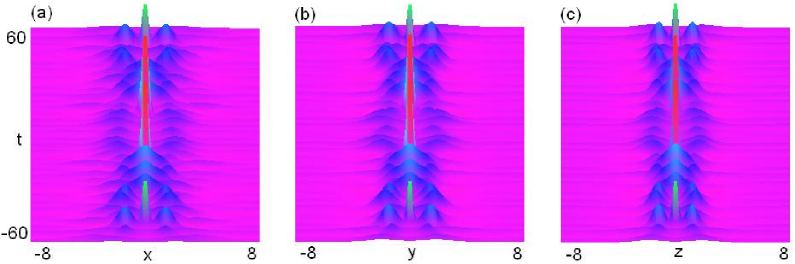
Figure 5: (color online). Color coded wave intensity (a) $|\Psi_{2}|^{2}(x,0,0,t)$ with $\max_{\{x,0,0,t\}}|\Psi_{2}|^{2}=0.135$, (b) $|\Psi_{2}|^{2}(0,y,0,t)$ with $\max_{\{0,y,0,t\}}|\Psi_{2}|^{2}=0.13$ and (c) $|\Psi_{2}|^{2}(0,0,z,t)$ with $\max_{\{0,0,z,t\}}|\Psi_{2}|^{2}=0.125$ given by the solution (25) for $a_{\sigma}(t)=0$ and other parameters given by Eq. (20) with $k_{x}=0.9,\,k_{y}=0.6,\,k_{z}=0.1$ and $k=0.6$.

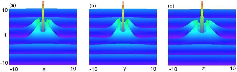
Figure 6: (color online). Color coded wave intensity (a) $|\Psi_{2}|^{2}(x,0,0,t)$ with $\max_{\{x,0,0,t\}}|\Psi_{2}|^{2}=0.038$, (b) $|\Psi_{2}|^{2}(0,y,0,t)$ with $\max_{\{0,y,0,t\}}|\Psi_{2}|^{2}=0.036$ and (c) $|\Psi_{2}|^{2}(0,0,z,t)$ with $\max_{\{0,0,z,t\}}|\Psi_{2}|^{2}=0.038$ given by the solution (25) for $a_{\sigma}(t)=0$ and other parameters given by Eq. (24).

V Conclusions

In conclusion, we have presented similarity reductions of the (3+1)-dimensional inhomogeneous nonlinear Schrödinger equation with variable coefficients to (1+1)-dimensional one with constant coefficients. This transformation allows us to relate certain class of localized solutions of the (3+1)-dimensional case to the variety of solutions of integrable NLS equation of (1+1)-dimensional case. As an example, we illustrated our technique by two lowest order rational solutions of the NLSE. These are transformed into rogue wave solutions localized in 3D space that have complicated evolution in time. The technique may also be extended to other NLS-type equations to exhibit their rogue wave solutions.

- (1) G. W. Bluman and S. Kumei, Symmetries and differential equations (Springer-Verlag, New York, 1989); P. J. Olver, Application of Lie groups to differential equations (2nd Ed.) (Springer-Verlag, New York, 1993); G. W. Bluman, A. Cheviakov, and S. Anco, Applications of symmetry methods to partial differential equations (Springer, New York, 2009); G. W. Bluman and Z. Y. Yan, Euro. J. Appl. Math. 16, 239 (2005).
- (2) M. Ablowitz and H. Segur, Solitons and the inverse scattering transform (SIAM, Philadelphia, 1981).
- (3) R. Y. Chiao, E. Garmair and C. H. Townes, Phys. Rev. Lett., 13, 479 (1964).
- (4) V. N. Vlasov, I. A. Petrishev and V. I. Talanov, Izv. Vyssh. Uchebn. Zaved., Radiofiz., 14, 1353 (1971).
- (5) L. Berge, Phys. Rep. 303, 259 (1998).
- (6) C. A. Akhmanov and R. V. Khokhlov, Problems of Nonlinear optics: Electromagnetic waves in nonlinear dispersive media, (VINITI, Moscow, 1964).
- (7) L. Gagnon, JOSA B 7, 1098 (1990).
- (8) Y. S. Kivshar, G. P. Agrawal, Optical solitons: from fibers to photonic crystals (Academic Press, New York, 2003). B. A. Malomed, D. Mihalache, F. Wise, and L. Torner, J. Opt. B: Quantum Semiclassical OPt. 7, 53R (2005).
- (9) L. Pitaevskii and S. Stringari, Bose-Einstein condensation (Oxford University Press, Oxford, 2003); R. Carretero-González, D. J. Frantzeskakis, and P. G. Kevrekidis, Nonlinearity 21, R139 (2008); F. Dalfovo, S. Giorgini, L. P. Pitaevskii, and S. Stringari, Rev. Mod. Phys. 71, 463 (1999); A. J. Legge, Rev. Mod. Phys. 73, 307 (2001).
- (10) Z. Y. Yan and V. V. Konotop, Phys. Rev. E 80, 036607 (2009).
- (11) Z. Y. Yan and C. Hang, Phys. Rev. A 80, 063626 (2009).
- (12) A. R. Osborne, Nonlinear ocean waves, (Academic Press, 2009).
- (13) A. Montina, U. Bortolozzo, S. Residori, and F. T. Arecchi, Phys. Rev. Lett., 103, 173901 (2009)
- (14) M. Shats, H. Punzmann, and H. Xia, Phys. Rev. Lett., 104, 104503 (2010).
- (15) D. R. Solli, C. Ropers, P. Koonath and B. Jalali, Nature 450, 1054 (2007); D. R. Solli, C. Ropers, and B. Jalali, Phys. Rev. Lett. 101, 233902 (2008).
- (16) D.-I. Yeom and B. Eggleton, Nature, 450, 953 (2007).
- (17) Yu. V. Bludov, V. V. Konotop and N. Akhmebiev, Opt. Lett. 34, 3015 (2009).
- (18) Z. Y. Yan, Phys. Lett. A 374, 672 (2010).
- (19) Yu. V. Bludov, V. V. Konotop, and N. Akhmediev, Phys. Rev. A, 80, 033610 (2009).
- (20) L. Stenflo and M. Marklund, J. Plasma Phys. 76, 293 (2010).
- (21) Z. Y. Yan, e-print arXiv:0911.4259, 2009.
- (22) J. Belmonte-Beitia, V. M. Pérez-García, V. Vekslerchik, and V. V. Konotop, Phys. Rev. Lett. 100, 164102 (2008).
- (23) N. Akhmediev, A. Ankiewicz, and J. M. Soto-Crespo, Phys. Lett. A 373, 2137 (2009).
- (24) N. Akhmediev, A. Ankiewicz, and M. Taki, Phys. Lett. A 373, 675 (2009). See also: N. Akhmediev, V. M. Eleonskii, and N. E. Kulagin, Sov. Phys. JETP 89, 1542 (1985).
- (25) N. Akhmediev, J. M. Soto-Crespo, and A. Ankiewicz, Phys. Rev. E 80, 026601 (2009).
- (26) A. Ankiewicz, P. A. Clarkson, and N. Akhmediev, J. Phys. A 43, 122002 (2010).