Spin structure of the pion from the instanton vacuum

Abstract

We investigate the spin structure of the pion within the framework of the nonlocal chiral quark model from the instanton vacuum. We first evaluate the tensor form factors of the pion for the first and second moment $(n=1,2)$ and compare it with the lattice data. Combining the tensor form factor of the pion with the electromagnetic one, we determine the impact-parameter dependent probability density of transversely polarized quarks inside the pion. It turns out that the present numerical results for the tensor form factor as well as those for the probability density are in good agreement with the lattice data. We also discuss the distortion of the spatial distribution of the quarks in the transverse plane inside the pion.

I Introduction

The transversity of hadrons has been one of the most important issues well over decades (see a recent review Barone:2001sp ), since it allows one to get access to their spin structures. It is pertinent to the tensor current of hadrons and is very difficult to be measured experimentally, because there is no direct probe to measure it. Only very recently, it was suggested that the transverse spin asymmetry $A_{TT}$ in Drell-Yan processes in $p\overline{p}$ reactions Efremov:2004 ; Anselimo:2004 ; PAX:2005 ; Pasquini:2006 as well as the azimuthal single spin asymmetry in semi-inclusive deep inelastic scattering (SIDIS) Anselmino:tensorcharge can be used to obtain information on the transversity of the nucleon. Though it is even more difficult to measure the transversity of the pion experimentally, it is still of great significance to understand it, since it provides the internal spin structure due to quarks, i.e. it accommodates a novel concept called a hadron tomography. The first result of the pion transversity on lattice has been reported by the QCDSF/UKQCD Collaborations Brommel:2007xd . They also presented the probability density of the polarized quarks inside the pion, combining the electromagnetic form factor of the pion Brommel:2006ww with its tensor form factor. It was shown in Ref. Brommel:2007xd that when the quarks are transversely polarized, their spatial distribution is strongly distorted. This first result in the lattice QCD has triggered several subsequent theoretical works Frederico:2009fk ; Gamberg:2009uk ; Broniowski:2010nt . In Ref. Broniowski:2010nt , the tensor form factors of the pion have been studied within the local and nonlocal Nambu-Jona-Lasinio (NJL) model Broniowski:2010nt , a direct comparison with the lattice results being emphasized. In doing so, they employed a larger value of the pion mass, i.e. $m_{\pi}=600$ MeV such that the results can be confronted with the lattice data. They also considered the case of the chiral limit.

In the present work, we first want to investigate the pion tensor form factor in the space-like momentum transfer region ($0\leq Q^{2}\leq 1$ GeV), based on the low-energy effective chiral action (E$\chi$A) from the instanton vacuum Diakonov:1985eg . Combining the result of the tensor form factor with the electromagnetic one of the pion which was already studied in Ref. Nam:2007gf within the same framework, we then derive the probability density of transversely polarized quarks inside the pion. Since the instanton vacuum realizes the spontaneous chiral symmetry breaking (S$\chi$SB) naturally via quark zero modes, it may provide a good framework to study properties of the pion such as the electromagnetic and tensor form factors. Moreover, an important merit of this approach lies in the fact that there are only two parameters, that is, the average (anti)instanton size $\bar{\rho}\approx 1/3$ fm and average inter-instanton distance $\bar{R}\approx 1$ fm. The normalization point is given by the average size of instantons and is approximately equal to $\rho^{-1}\approx 0.6$ GeV. The values of the $\bar{\rho}$ and $\bar{R}$ were estimated many years ago phenomenologically in Ref. Shuryak:1981ff as well as theoretically in Ref. Diakonov:1983hh ; Diakonov:2002fq ; Schafer:1996wv . The instanton framework has been proved to be reliable in reproducing experimental data especially for the meson sector, such as the meson distribution amplitudes Nam:2006sx ; Nam:2006mb ; Nam:2006au , semileptonic decays Nam:2007fx , and etc. Furthermore, this approach was supported by various lattice simulations of the QCD vacuum Chu:vi ; Negele:1998ev ; DeGrand:2001tm . The quark propagator from the instanton vacuum  Diakonov:1983hh is in a remarkable agreement with lattice calculations Faccioli:2003qz ; Bowman:2004xi . Finally the nonlocal chiral quark model from the instanton vacuum has a practical virtue, since it does not have any adjustable parameter once the above-mentioned two parameters $\bar{\rho}$ and $\bar{R}$ are determined.

We organize the present work as follows: In Section II, we briefly explain the definitions of the probability densities of the transversely polarized quarks, which are expressed in terms of generalized form factors of the pion. In Section III, we show how to calculate the tensor form factors within the nonlocal chiral quark model from the instanton vacuum. In Section IV, the numerical results are discussed and compared with those in lattice QCD. The final Section is devoted to summarize the present work, to draw conclusions, and to give outlook.

II Generalized form factors of the pion

In this Section, we define the probability density of transversely polarized quarks inside the pion. For definiteness, we choose the positively charged pion $\pi^{+}$ from now on. The probability density of transversely polarized quarks for the $n$ th moment of the probability density is given as

$$\rho_{n}(b_{\perp},s_{\perp})=\int^{1}_{-1}dx\,x^{n-1}\rho(x,b_{\perp},s_{\perp})=\frac{1}{2}\left[A_{n0}(b^{2}_{\perp})-\frac{s^{i}_{\perp}\epsilon^{ij}b^{j}_{\perp}}{m_{\pi}}\frac{\partial B_{n0}(b^{2}_{\perp})}{\partial b^{2}_{\perp}}\right],$$ (1)

where $b_{\perp}$ denote the impact parameter that measures the distance from the center of momentum of the pion to the quark in the transverse plane to its motion. The $s_{\perp}$ stands for the fixed transverse spin of the quark. For simplicity, we choose the $z$ direction for the quark longitudinal momentum. The $x$ indicates the momentum fraction possessed by the quark inside the pion. The $A_{n0}(b_{\perp}^{2})$ and $B_{n0}(b_{\perp}^{2})$ are called the generalized form factors (GFFs). In fact, the GFFs are just the moments of the generalized parton distributions (GPDs) for the unpolarized and transversely polarized pions, respectively:

$$\int^{1}_{-1}dx\,x^{n-1}H(x,\xi=0,b^{2}_{\perp})=A_{n0}(b^{2}_{\perp}),\,\,\,\,\int^{1}_{-1}dx\,x^{n-1}E(x,\xi=0,b^{2}_{\perp})=B_{n0}(b^{2}_{\perp}).$$ (2)

For the first moment, the GFFs $A_{10}$ and $B_{10}$ are identified with the electromagnetic and tensor form factors of the pion, respectively. Previously, we have studied $A_{10}(q^{2})$ in the momentum space within the nonlocal chiral quark model (NL$\chi$QM) from the instanton vacuum Nam:2007gf , resulting in a good agreement with the experimental data. Hence, we can readily calculate $A_{10}(b_{\perp})$, using the results of Ref. Nam:2007gf . Thus, we will concentrate on calculating the tensor form factors $B_{10,20}$ within the same framework, and they can be written in a general form as follows:

$$\langle\pi^{+}(p_{f})|\mathcal{O}^{\mu\nu\mu_{1}\cdots\mu_{n-1}}_{T}|\pi^{+}(p_{i})\rangle=\mathcal{AS}\left[\frac{(p^{\mu}q^{\nu}-q^{\mu}p^{\nu})}{m_{\pi}}\sum^{n-1}_{i=\mathrm{even}}q^{\mu_{1}}\cdots q^{\mu_{i}}p^{\mu_{i+1}}\cdots p^{\mu_{n-1}}B_{ni}(Q^{2})\right],$$ (3)

where $p_{i}$ and $p_{f}$ stand for the initial and final on-shell momenta of the pion, respectively. We also use notations $p=(p_{f}+p_{i})/2$ and $q=p_{f}-p_{i}$. The tensor operator also can be given as:

$$\mathcal{O}^{\mu\nu\mu_{1}\cdots\mu_{n-1}}_{T}=\mathcal{AS}\left[q^{\dagger}\sigma^{\mu\nu}(i\tensor{D}^{\mu_{1}})\cdots(i\tensor{D}^{\mu_{n-1}})q\right].$$ (4)

The $\mathcal{A}$ and $\mathcal{S}$ denote the anti-symmetrization in $(\mu,\nu)$ and symmetrization in $(\nu,\cdots,\mu_{n-1})$ with the trace terms subtracted in all the indices. Taking into account Eqs. (3) and (4), we can define the tensor form factors $B_{10}$ and $B_{20}$ of the pion in momentum space as the matrix elements of the tensor current, using the auxiliary-vector method as in Ref. Diehl:2010ru :

$$\langle\pi^{+}(p_{f})|q^{\dagger}(0)\sigma_{ab}q(0)|\pi^{+}(p_{i})\rangle=\left[(p_{i}\cdot a)(p_{f}\cdot b)-(p_{i}\cdot b)(p_{f}\cdot a)\right]\frac{B_{10}(Q^{2})}{m_{\pi}},$$ (5)

$$\langle\pi^{+}(p_{f})|q^{\dagger}(0)\sigma_{ab}(i\tensor{D}\cdot a)q(0)|\pi^{+}(p_{i})\rangle=\left\{(p\cdot a)[(p_{i}\cdot a)(p_{f}\cdot b)-(p_{i}\cdot b)(p_{f}\cdot a)]\right\}\frac{B_{20}(Q^{2})}{m_{\pi}},$$ (6)

where the vectors satisfy the conditions, i.e. $a^{2}=0$, $a\cdot b=0$ and $b^{2}\neq 0$, and we have used a notation $\sigma_{ab}\equiv\sigma_{\mu\nu}a^{\mu}b^{\nu}$. Due to this auxiliary-vector method, one can eliminate the trace-term subtractions. We also introduce a notation $i\tensor{D}_{\mu}\equiv(i\roarrow{D}_{\mu}-i\loarrow{D}_{\mu})/2$, where $D_{\mu}$ indicates the SU($N_{c}$) covariant derivative. Since we are interested in the spatial distribution of the transversely polarized quark inside the pion, we need to consider the Fourier transform of the form factors:

$$F(b^{2}_{\perp})=\frac{1}{(2\pi)^{2}}\int d^{2}q_{\perp}e^{-ib_{\perp}\cdot q_{\perp}}F(q^{2}_{\perp})=\frac{1}{2\pi}\int^{\infty}_{0}QdQJ_{0}(bQ)F(Q^{2}),$$ (7)

where $F=(A_{10},B_{10})$ designates the generic pion form factor. The magnitudes of the transverse momentum and impact parameter are expressed as $|\bm{q}_{\perp}|\equiv Q$ and $|\bm{b}_{\perp}|\equiv b$. Similarly, the Fourier transform of the derivative of the GFF with respect to $b^{2}_{\perp}$ can be evaluated as:

$$\frac{\partial F(b^{2}_{\perp})}{\partial b^{2}_{\perp}}\equiv F^{\prime}(b^{2}_{\perp})=-\frac{1}{4\pi b}\int^{\infty}_{0}Q^{2}dQJ_{1}(bQ)F(Q^{2}).$$ (8)

The $J_{0}$ and $J_{1}$ in Eqs.(7,8) denote the Bessel functions of order $0$ and $1$, respectively. According to the definitions for the relevant vectors $q_{\perp}$ and $b_{\perp}$, the probability density in Eq. (1) reads as follows:

$$\rho_{1}\left(b_{\perp},s_{x}=\pm 1\right)=\frac{1}{2}\left[A_{10}(b^{2})\mp\frac{b\sin\theta_{\perp}}{m_{\pi}}B^{\prime}_{10}(b^{2})\right],$$ (9)

where the spin of the quark inside the pion is quantized along the $x$ axis, $s_{\perp}=(\pm 1,0)$.

III Nonlocal chiral quark model from the instanton vacuum

We now briefly explain the NL$\chi$QM from the instanton vacuum Diakonov:1995qy and derive the GFFs of the pion. Considering first the dilute instanton liquid, characterized by the average (anti)instanton size $\bar{\rho}\approx 1/3$ fm and average inter-instanton distance $\bar{R}\approx 1$ fm with the small packing parameter $\pi\bar{\rho}^{4}/\bar{R}^{4}\approx 0.1$, we are able to average the fermionic determinant over collective coordinates of instantons with fermionic quasi-particles, i.e. the constituent quarks introduced. The averaged determinant is reduced to the light-quark partition function that can be given as a functional of the tensor field in the present case. Having bosonized and integrated it over the quark fields, we obtain the following effective nonlocal chiral action in the large $N_{c}$ limit in Euclidean space:

$$\mathcal{S}_{\mathrm{eff}}[m,\pi]=-\mathrm{Sp}\ln\left[i\hbox to0.0pt{/\hss}{\partial}+im+i\sqrt{M(i\partial)}U^{\gamma_{5}}(\phi)\sqrt{M(i\partial)}+\sigma\cdot T\right],$$ (10)

where $m$, $\pi$, and $\mathrm{Sp}$ indicate the current quark mass, the Nambu-Goldstone (NG) boson field, and the functional trace over all relevant spaces, respectively. In the numerical calculations, we will choose $m\sim m_{u}\sim m_{d}\approx 5$ MeV, taking into account isospin symmetry. The $M(i\partial)$ stands for the momentum-dependent effective quark mass, generated from the nontrivial quark-(anti)instanton interactions Diakonov:1985eg . Although its analytical form is in general given by the modified Bessel functions, we will make use of its parametrization for numerical convenience:

$$M(i\partial)=M_{0}\left(\frac{2}{2+\bar{\rho}^{2}\partial^{2}}\right)^{2},$$ (11)

where $M_{0}$ indicates the constituent quark mass, which can be determined self-consistently by solving the gap equation of the present framework, resulting in $M_{0}=350$ MeV Diakonov:1985eg . The NG boson field is represented in a nonlinear form as Diakonov:1995qy :

$$U^{\gamma_{5}}(\phi)=\exp\left[\frac{i\gamma_{5}(\bm{\tau}\cdot\bm{\phi})}{F_{\phi}}\right]=1+\frac{i\gamma_{5}(\bm{\tau}\cdot\bm{\phi})}{F_{\phi}}-\frac{(\bm{\tau}\cdot\bm{\phi})^{2}}{2F^{2}_{\phi}}+\cdots,$$ (12)

where $\phi^{a}$ is the SU(2) multiplet, defined as

$$\bm{\tau}\cdot\bm{\phi}=\left(\begin{array}[]{cc}\frac{\pi^{0}}{\sqrt{2}}&\pi^{+}\\ \pi^{-}&\frac{\pi^{0}}{\sqrt{2}}\\ \end{array}\right).$$ (13)

The $F_{\phi}$ denotes the weak-decay constant for NG bosons, whose empirical value is $93.2$ MeV for the pion for instance. The last term in Eq. (10) denotes $\sigma\cdot T=\sigma_{\mu\nu}T_{\mu\nu}$, where $\sigma_{\mu\nu}=i[\gamma_{\mu},\,\gamma_{\nu}]/2$ and $T_{\mu\nu}$ represents the external tensor source field.

The three-point correlation function in Eq. (5) can be easily calculated by a functional differentiation with respect to the pion and external tensor fields, which leads to the following two terms for the $B_{10}(Q^{2})$:

$$\frac{\delta^{3}\mathcal{S}_{\mathrm{eff}}[m,\pi,T]}{\delta T\,\delta\pi^{a}\delta\pi^{b}}\Big{|}_{T=0}=-\frac{1}{F^{2}_{\pi}}\mathrm{Sp}\left[\frac{1}{i\hbox to0.0pt{\,/\hss}{D}}\sqrt{M}\gamma_{5}\tau^{a}\sqrt{M}\frac{1}{i\hbox to0.0pt{\,/\hss}{D}}\sqrt{M}\gamma_{5}\tau^{b}\sqrt{M}\frac{1}{i\hbox to0.0pt{\,/\hss}{D}}\sigma_{\mu\nu}\right]-\frac{i}{2F^{2}_{\pi}}\mathrm{Sp}\left[\frac{1}{i\hbox to0.0pt{\,/\hss}{D}}\sqrt{M}\tau^{a}\tau^{b}\sqrt{M}\frac{1}{i\hbox to0.0pt{\,/\hss}{D}}\sigma_{\mu\nu}\right],$$ (14)

where we have introduced the shorthand notations $M=M(i\partial)$ and $i\hbox to0.0pt{\,/\hss}{D}=i\hbox to0.0pt{/\hss}{\partial}+im+iM(i\partial)=i\hbox to0.0pt{/\hss}{\partial}+i\bar{M}(i\partial)$. The trace over the isospin space yields $\mathrm{tr}_{\tau}[\tau^{a}\tau^{b}]=2\delta^{ab}$. One can also do for the $B_{20}(Q^{2})$ similarly. Having performed the functional trace and the trace over the color space, we arrive at the matrix elements for the $B_{(10,20)}(Q^{2})$, corresponding to Eq. (5), as follows:

$$\langle\pi^{+}(p_{f})|q^{\dagger}(0)\sigma_{ab}q(0)|\pi^{+}(p_{i})\rangle = \underbrace{-\frac{2N_{c}}{F^{2}_{\pi}}\int\frac{d^{4}k}{(2\pi)^{4}}\mathrm{Tr}_{\gamma}\left[\frac{1}{i\hbox to0.0pt{\,/\hss}{D}_{a}}\sqrt{M_{a}}\gamma_{5}\sqrt{M_{b}}\frac{1}{i\hbox to0.0pt{\,/\hss}{D}_{b}}\sqrt{M_{b}}\gamma_{5}\sqrt{M_{c}}\frac{1}{i\hbox to0.0pt{\,/\hss}{D}_{c}}\sigma_{ab}\right]}_{\mathrm{(A)}}$$ (16)

$$\underbrace{-\frac{iN_{c}}{F^{2}_{\pi}}\int\frac{d^{4}k}{(2\pi)^{4}}\mathrm{Tr}_{\gamma}\left[\frac{1}{i\hbox to0.0pt{\,/\hss}{D}_{b}}\sqrt{M_{b}}\frac{1}{i\hbox to0.0pt{\,/\hss}{D}_{c}}\sqrt{M_{c}}\sigma_{ab}\right]}_{\mathrm{(B)}},$$

$$\langle\pi^{+}(p_{f})|q^{\dagger}(0)\sigma_{ab}(i\tensor{D}\cdot a)q(0)|\pi^{+}(p_{i})\rangle = \underbrace{-\frac{2N_{c}}{F^{2}_{\pi}}\int\frac{d^{4}k}{(2\pi)^{4}}\mathrm{Tr}_{\gamma}\left[\frac{1}{i\hbox to0.0pt{\,/\hss}{D}_{a}}\sqrt{M_{a}}\gamma_{5}\sqrt{M_{b}}\frac{1}{i\hbox to0.0pt{\,/\hss}{D}_{b}}\sqrt{M_{b}}\gamma_{5}\sqrt{M_{c}}\frac{1}{i\hbox to0.0pt{\,/\hss}{D}_{c}}\sigma_{ab}[(k+\frac{p_{i}}{2})\cdot a]\right]}_{\mathrm{(A)}}$$ (18)

$$\underbrace{-\frac{iN_{c}}{F^{2}_{\pi}}\int\frac{d^{4}k}{(2\pi)^{4}}\mathrm{Tr}_{\gamma}\left[\frac{1}{i\hbox to0.0pt{\,/\hss}{D}_{b}}\sqrt{M_{b}}\frac{1}{i\hbox to0.0pt{\,/\hss}{D}_{c}}\sqrt{M_{c}}\sigma_{ab}[(k+\frac{p_{i}}{2})\cdot a]\right]}_{\mathrm{(B)}}.$$

The corresponding Feynman diagrams to the two terms (A) and (B) in the right-hand side of Eq. (16) are depicted in Fig. 1, respectively.

Figure 1: Feynman diagrams for $B_{n0}$ in the NL$\chi$QM. We assign the initial and final pion momenta as $p_{i}$ and $p_{f}$, respectively, while the momentum transfer as $q$. We also define the loop momenta as $k_{a}=k-\frac{p_{i}}{2}-\frac{q}{2}$, $k_{b}=k+\frac{p_{i}}{2}-\frac{q}{2}$, and $k_{c}=k+\frac{p_{i}}{2}+\frac{q}{2}$.

The relevant momenta are also defined as:

$$k_{a} = k-\frac{p_{i}}{2}-\frac{q}{2},\,\,\,\,k_{b}=k+\frac{p_{i}}{2}-\frac{q}{2},\,\,\,\,k_{c}=k+\frac{p_{i}}{2}+\frac{q}{2}.$$ (19)

In order to evaluate the matrix element, we define the initial and final pion momenta in the Breit (brick-wall) frame in Euclidean space as done in Ref. Nam:2007gf :

$$p_{i}=\left(-\frac{Q}{2},0,0,i\sqrt{\frac{Q^{2}}{4}+m^{2}_{\pi}}\right),\,\,\,\,p_{f}=\left(\frac{Q}{2},0,0,i\sqrt{\frac{Q^{2}}{4}+m^{2}_{\pi}}\right),\,\,\,\,q=\left(Q,0,0,0\right).$$ (20)

We also have chosen the auxiliary vectors for definiteness as $a=(0,1,0,i)$ and $b=(1,0,1,0)$, which satisfy the conditions mentioned in Section II. The denominators become $\hbox to0.0pt{\,/\hss}{D}_{a,b,c}=\hbox to0.0pt{/\hss}{k}_{a,b,c}+i\bar{M}_{a,b,c}$ in Eq. (16). The momentum-dependent effective quark mass $M_{a,b,c}$ can be also defined by using Eqs. (11) and (19).

IV Numerical results and Discussions

We first discuss the numerical results of the tensor form factors of the pion. Figure 2 draws the numerical results for the electromagnetic form factor of the pion $A_{10}$ in the left panel and its tensor form factor $B_{10}$ in the right panel as functions of $Q^{2}$ in the range of $0\leq Q^{2}\leq 1\,\mathrm{GeV}^{2}$.

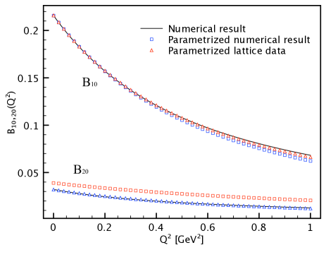
Figure 2: The numerical results for the electromagnetic form factor $A_{10}(Q^{2})$ are presented in the left panel and those for the tensor form factors $B_{10}(Q^{2})$ and $B_{20}(Q^{2})$ in the right panel. The solid curves depict the numerical results, whereas their parametrizations given respectively in Eqs. (21) and (25) are denoted by the squares. We also show the parametrized lattice data Brommel:2007xd for the tensor form factors, designated by the triangles in the right panel.

However, we want to mention that there is a caveat. Since we need the results of the form factors in principle up to infinite $Q^{2}$ in order to perform the Fourier transform given in Eq. (7), we will use the parametrized one, as we will discuss later in the context of the lattice data.

The numerical results for $A_{10}(Q^{2})$ are taken from Ref. Nam:2007gf . Though we have already discussed those for the electromagnetic form factor in detail in Ref. Nam:2007gf , we want to recapitulate them in the context of the lattice data. It is well known that the electromagnetic form factor can be parametrized by a monopole form

$$F_{\pi}(Q^{2})=A_{10}(Q^{2})=\frac{1}{1+Q^{2}/M^{2}}.$$ (21)

The monopole mass $M$ was known to be $M=(0.714\pm 0.004)$ GeV, based on the experimental data Amendolia:1986wj ; Tadevosyan:2007yd ; Horn:2006tm . On the other hand, the lattice calculation yields $M=(0.727\pm 0.016)$ GeV with a linear chiral extrapolation to the physical pion mass taken into account Brommel:2006ww . The present result leads to $M=0.738\,\mathrm{GeV}$, which indicates that that of the pion electromagnetic form factor is in good agreement with the lattice data. We also obtain the squared charge radius of the pion $\langle r^{2}\rangle=0.456\,\mathrm{fm}^{2}$, while in the lattice QCD it was evaluated to be $\langle r^{2}\rangle=(0.441\pm 0.019)\,\mathrm{fm}^{2}$. Considering the uncertainty of the lattice data, the present result is in remarkable agreement with them. In the left panel of Fig. 2, we show the numerical result (solid curve) Nam:2007gf and its monopole parametrization (sqaure) of $A_{10}(Q^{2})$, using the values mentioned above and Eq. (21).

In the right panel of Fig. 2, we draw the numerical results for the tensor form factors $B_{10}(Q^{2})$ and $B_{20}(Q^{2})$ (solid curve). In order to compare the present results with the lattice data, it is crucial to consider the evolution of the scale Barone:2001sp ; Broniowski:2009zh ; Broniowski:2010nt , since the tensor current is not the conserved one. The tensor form factor is evolved at the leading order (LO) by the following equation Barone:2001sp ; Broniowski:2010nt

$$B_{n0}(Q^{2},\mu)=B_{n0}(Q^{2},\mu_{0})\left[\frac{\alpha(\mu)}{\alpha(\mu_{0})}\right]^{{\gamma_{n}}/{(2\beta_{0})}},$$ (22)

where we have used the anomalous dimensions $\gamma_{1}=8/3$ and $\gamma_{2}=8$, and $\beta_{0}=11N_{c}/3-2N_{f}/3$ ($N_{c}=3$ and $N_{f}=2$ in the present case). Thus, the powers in the LO evolution equation are given as $4/29$ and $12/29$ respectively for $n=1$ and $n=2$, which indicate that the dependence of the tensor charge on the normalization point turns out to be rather weak. Note that the anomalous dimension is simply the same as that for the nucleon tensor charge Kim:1995bq . We also take $\Lambda_{\mathrm{QCD}}=0.248\,\mathrm{GeV}$ which was also used in evolving the nucleon tensor charges and tensor anomalous magnetic moments Ledwig:2010tu ; Ledwig:2010zq . Since the normalization point of the present model is around $0.6\,\mathrm{GeV}$, while the lattice calculation was carried out at $\mu=2\,\mathrm{GeV}$, the scale factors turn out to be

$$B_{10}(Q^{2},\mu=2\,\mathrm{GeV})=0.89\,B_{10}(Q^{2},\mu_{0}=0.6\,\mathrm{GeV}),\;\;\;\;B_{20}(Q^{2},\mu=2\,\mathrm{GeV})=0.70\,B_{20}(Q^{2},\mu_{0}=0.6\,\mathrm{GeV}).$$ (23)

Considering these scalings, we obtain $B_{10}(0)=0.216$ and $B_{20}(0)=0.032$. In the lattice calculation Brommel:2007xd , the tensor charge of the pion for $n=1$ with the linear chiral extrapolation to the physical pion mass in $m_{\pi}^{2}$ was estimated to be about $B_{10}(0)=0.216$, which is almost identical to the present result. As for $n=2$, the lattice data estimated about $B_{20}(0)=0.039$, which is about $20\,\%$ larger than the present one, but is still comparable. We want to mention that one could use larger current-quark masses in order to compare directly with the lattice data as done in Ref. Broniowski:2010nt . However, it is rather unreliable in the present framework: Firstly it is nontrivial to include the larger current quark mass Musakhanov:1998wp ; Musakhanov:2002vu ; Musakhanov:2002xa . Secondly, the present scheme is conceptually only valid when the current quark mass is small, at least up to the strange current quark mass. Thus, the NL$\chi$QM from the instanton vacuum is a rather restricted one, so that we will compare the present results with those of the lattice QCD with chiral extrapolation.

In Fig. 3, we present the $m_{\pi}$ dependence of the pion tensor form factor scaled by the pion mass as a function of $m^{2}_{\pi}$ for $m_{\pi}=0$ (square) and $140$ MeV (circle). As shown in Fig. 3, the result in the chiral limit is slightly smaller than that with $m_{\pi}=140\,\mathrm{MeV}$. As for the case with $m_{\pi}=0$, we take the current quark mass $m=0$. The shaded bands represent the fits from the lattice calculation Brommel:2007xd .

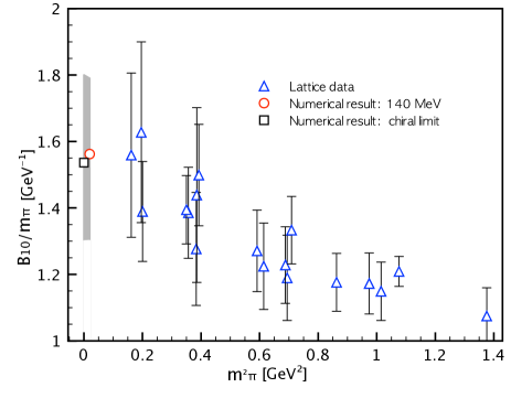
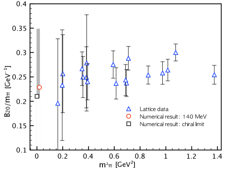
Figure 3: $B_{10}(0)/m_{\pi}$ (left) and $B_{20}(0)/m_{\pi}$ (right) as functions of $m^{2}_{\pi}$. The numerical results for $m_{\pi}=0$ and $140$ MeV are given by the square and circle. The lattice data (triangle) are taken from Ref. Brommel:2007xd . The shaded areas for $m_{\pi}=(0\sim 140)$ MeV represent the lattice fits.

A simple $p$-pole parametrization of GFFs was used in Ref. Brommel:2007xd to get the tensor form factor of the pion:

$$B_{n0}(Q^{2})=B_{n0}(0)\left[1+\frac{Q^{2}}{p_{n}\,m^{2}_{p_{n}}}\right]^{-p_{n}}.$$ (24)

In this parametrization, the lattice QCD simulation estimated the pole mass $m_{p_{1}}=(0.756\pm 0.095)$ GeV and $m_{p_{2}}=(1.130\pm 0.265)$ at $m_{\pi}=140$ MeV with chiral extrapolation. Considering the condition $p>1.5$ for the regular behavior of the probability density at $b_{\perp}\to 0$ Diehl:2005jf and following Ref. Brommel:2007xd , we take $p_{1}=p_{2}=1.6$ as a trial. If this is the case, Eq. (24) gives us $m_{p_{1}}\approx 0.761$ GeV and $m_{p_{2}}\approx 0.864$ GeV to reproduce the present results, which is compatible with that of the lattice simulation. Taking into account these results, we can write the $p$-pole parametrized tensor form factor as follows:

$$B_{10}(Q^{2})=0.216\left[1+\frac{Q^{2}}{1.6\times 0.761^{2}\,\mathrm{GeV}^{2}}\right]^{-1.6},\,\,\,\,B_{20}(Q^{2})=0.032\left[1+\frac{Q^{2}}{1.6\times 0.864^{2}\,\mathrm{GeV}^{2}}\right]^{-1.6},$$ (25)

The result of this parametrized one in Eq. (25) is also depicted in the right panel of Fig. 2 (square), and reproduces well the present numerical one. We also compare our result with the lattice one in the right panel of Fig. 2. As in the case of the electromagnetic form factors, the present results are in excellent agreement with the lattice data (triangle). Note that in the present framework we do not have any adjustable free parameter.

We are now in a position to discuss the results of the probability densities of the transversely polarized quarks inside the pion, defined in Eq. (1). In the upper-left panel of Fig. 4, we show the unpolarized probability density with the tensor form factor turned off. As expected, the quarks are distributed symmetrically on the $b_{x}$-$b_{y}$ plane. On the other hand, if we switch on the tensor form factor, the spatial distribution of a transversely polarized quark inside the pion ($\pi^{+}$) gets distorted as shown in the upper-right panel of Fig. 4.

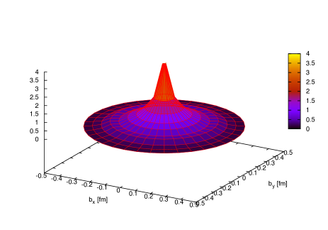
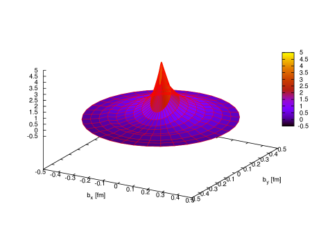
Figure 4: In the upper panels, we show unpolarized (left) and polarized (right) probability densities, $\rho_{1}$ in Eq. (1) as a function of $b_{x}$ and $b_{y}$ for $s_{\perp}=(+1,0)$. Similarly, we show their three dimensional profiles in the lower panels.

Its maximum value is also shifted to the $b_{y}$ direction in comparison to that for the unpolarized one. Thus, it is interesting to examine the average transverse shift which is defined as Brommel:2007xd :

$$\langle b_{y}\rangle=\frac{\int d^{2}\,b_{\perp}\,b_{y}\,\rho(b_{\perp},s_{\perp})}{\int d^{2}\,b_{\perp}\,\rho(b_{\perp},s_{\perp})}=\frac{1}{2m_{\pi}}\frac{B_{10}(0)}{A_{10}(0)},$$ (26)

where we have chosen $s_{\perp}=(+1,0)$. Using Eq. (25) and $m_{\pi}=140$ MeV, we obtain $\langle b_{y}\rangle=0.152$ fm, which is almost the same as that of the lattice calculation $\langle b_{y}\rangle=(0.151\pm 0.024)$ fm. This finite value of $\langle b_{y}\rangle$ measures how much the polarized probability density is distorted in the transverse plane. If we take the spin quantized along the $y$ axis, i.e. $s_{\perp}=(0,+1)$, the result of the polarized probability density is similar but rotated by $90^{\circ}$ clockwise. We also note that the present results are almost equivalent to those given by the lattice simulation Brommel:2007xd . In the lower panel of Fig. 4, we show the three-dimensional profiles for the unpolarized (left) and transversely polarized (right) distributions as functions of $b_{x}$ and $b_{y}$. One can obviously see that the maximum of the transversely polarized probability density is shifted and distorted.

In Fig. 5, we draw the probability density as a function of $b_{y}$ at $b_{x}\approx 0.2$ fm, comparing it with that of the lattice calculation. As expected, the present result is almost identical to that of the lattice QCD. We summarize the main results of the present work in Table 1:

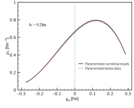
Figure 5: Comparison between the polarized probability densities from the present (square) and lattice (triangle) results for $b_{x}\approx 0.2$ fm.

$m_{\pi}=140$ MeV	$B_{10}(0)$	$m_{p_{1}}$ [GeV]	$\langle b_{y}\rangle$ [fm]	$B_{20}(0)$	$m_{p_{2}}$ [GeV]
Present work	$0.216$	$0.762$	$0.152$	$0.032$	$0.864$
Lattice QCD Brommel:2007xd	$0.216\pm 0.034$	$0.756\pm 0.095$	$0.151$	$0.039\pm 0.099$	$1.130\pm 0.265$

Table 1: Numerical results for $B_{n0}(0)$, $m_{p_{n}}$, and $\langle b_{y}\rangle$ in comparison with those of the lattice simulation Brommel:2007xd with the chiral extrapolation to the physical pion mass $m_{\pi}=140$ MeV.

V Summary and conclusion

In the present work, we have aimed at investigating the tensor form factors of the pion, $B_{10}$ and $B_{20}$, using the nonlocal chiral quark model from the instanton vacuum. Combining it with the electromagnetic form factor of the pion Nam:2007gf , we were able to evaluate the transversely polarized density of quarks inside the pion as functions of $(b_{x},b_{y})$ in comparison with the lattice simulation Brommel:2007xd .

We first recapitulated the electromagnetic form factor of the pion computed previously in the context of the lattice calculation. We found that the monopole mass is $M=0.738$ GeV which is in a good agreement with that from the lattice QCD $M=0.727$ GeV as well as the experimental data $M=(0.714\pm 0.004)$ GeV. It indicates that the $Q^{2}$ dependence of the electromagnetic form factor is well reproduced within the present work and compatible with the lattice results. We also presented the squared charge radius of the pion $\langle r^{2}\rangle=0.456\,\mathrm{fm}^{2}$ which is again in very good agreement with the lattice result $\langle r^{2}\rangle=(0.441\pm 0.019)\,\mathrm{fm}^{2}$.

We calculated the tensor form factor of the pion within the same framework as done in previous works. In order to compare the results with the lattice data, we evolved them from the $\mu=\bar{\rho}^{-1}=600\,\mathrm{MeV}$ to the scale at which the lattice calculation was performed ($\mu=2\,\mathrm{GeV}$). We also carried out the $p$-pole parametrization as in the lattice QCD. The results for the tensor form factor were obtained as follows: The tensor form factors of the pion at $Q^{2}=0$ $(B_{(10)}(0),\,B_{(20)}(0))=(0.216,\,0.032)$ and the pole mass $m_{p_{(1,2)}}=(0.762,0.864)\,\mathrm{GeV}$. Being compared to the lattice results with chiral extrapolation, i.e. $B_{(10,20)}(0)=(0.216\pm 0.034,0.039\pm 0.099)$ and $m_{p_{(1,2)}}=(0.756\pm 0.095,1.130\pm 0.265)$ GeV, they were found to be almost identical and comparable to those of the lattice QCD. In particular, these results are remarkable, considering the fact that the present scheme does not contain any adjustable parameter.

Having combined the results of the tensor form factor with those of the electromagnetic one, we obtained straightforwardly the probability density of transversely polarized quarks inside the pion. It turned out that the spatial distribution of the quarks on the transverse plane were distorted, compared to that of the unpolarized quarks. Moreover, the maximum value of the density is shifted to the $b_{y}$ direction. In order to examine this shift, we also calculated the average value of $b_{y}$ which turned out to be $\langle b_{y}\rangle=0.152\,\mathrm{fm}$. It is in an excellent agreement with the lattice result $\langle b_{y}\rangle=0.151\,\mathrm{fm}$.

Finally, It is worth mentioning that it is also of great importance to study the spin structure of the kaon, since it sheds light on the role of flavor SU(3) symmetry breaking inside the kaon. Related works are under progress and will appear elsewhere.

References

- (1) V. Barone, A. Drago and P. G. Ratcliffe, Phys. Rept. 359 (2002) 1.
- (2) A.V. Efremov, K. Goeke, and P. Schweitzer, Eur. Phys. J. C 35 (2004) 207.
- (3) V. Barone, [PAX Collaboration], hep-ex/0505054.
- (4) M. Anselmino, V. Barone, A. Drago, and N.N. Nikolaev, Phys. Lett. B 594 (2004) 97.
- (5) B. Pasquini, M. Pincetti, and S. Boffi, Phys. Rev. D 76 (2007) 034020.
- (6) M. Anselmino,M. Boglione, U. D’Alesio, A. Kotzinian, F. Murgia, A. Prokudin, and C. Turk, Phys. Rev. D 75 (2007) 054032.
- (7) D. Brommel et al. [QCDSF/UKQCD Collaboration], Phys. Rev. Lett. 101 (2008) 122001.
- (8) D. Brommel et al. [QCDSF/UKQCD Collaboration], Eur. Phys. J. C 51 (2007) 335.
- (9) T. Frederico, E. Pace, B. Pasquini and G. Salme, Phys. Rev. D 80 (2009) 054021.
- (10) L. Gamberg and M. Schlegel, Phys. Lett. B 685 (2010) 95.
- (11) W. Broniowski, A. E. Dorokhov and E. R. Arriola, Phys. Rev. D 82, 094001 (2010).
- (12) D. Diakonov and V. Y. Petrov, Nucl. Phys. B 272(1986) 457.
- (13) S. i. Nam and H. -Ch. Kim, Phys. Rev. D 77 (2008) 094014.
- (14) E. V. Shuryak, Nucl. Phys. B 203 (1982) 93.
- (15) D. Diakonov and V. Y. Petrov, Nucl. Phys. B 245 (1984) 259.
- (16) D. Diakonov, Prog. Part. Nucl. Phys. 51 (2003) 173.
- (17) T. Schäfer and E. V. Shuryak, Rev. Mod. Phys. 70 (1998) 323.
- (18) S. i. Nam and H. -Ch. Kim, Phys. Rev. D 74 (2006) 076005.
- (19) S. i. Nam and H. -Ch. Kim, Phys. Rev. D 74 (2006) 096007.
- (20) S. i. Nam, H. -Ch. Kim, A. Hosaka and M. M. Musakhanov, Phys. Rev. D 74 (2006) 014019.
- (21) S. i. Nam and H. -Ch. Kim, Phys. Rev. D 75 (2007) 094011.
- (22) M. C. Chu, J. M. Grandy, S. Huang and J. W. Negele, Phys. Rev. D 49 (1994) 6039.
- (23) J. W. Negele, Nucl. Phys. Proc. Suppl. 73 (1999) 92.
- (24) T. DeGrand, Phys. Rev. D 64 (2001) 094508.
- (25) P. Faccioli and T. A. DeGrand, Phys. Rev. Lett. 91 (2003) 182001.
- (26) P. O. Bowman et al. Nucl. Phys. Proc. Suppl. 128 (2004) 23.
- (27) M. Diehl, L. Szymanowski, Phys. Lett. B690, 149-158 (2010).
- (28) D. Diakonov, M. V. Polyakov and C. Weiss, Nucl. Phys. B 461 (1996) 539.
- (29) S. R. Amendolia et al. [NA7 Collaboration], Nucl. Phys. B 277 (1986) 168.
- (30) V. Tadevosyan et al. [Jefferson Lab F(pi) Collaboration], Phys. Rev. C 75 (2007) 055205.
- (31) T. Horn et al. [Jefferson Lab F(pi)-2 Collaboration], Phys. Rev. Lett. 97 (2006) 192001.
- (32) W. Broniowski and E. R. Arriola, Phys. Rev. D 79 (2009) 057501.
- (33) H.-Ch. Kim, M. V. Polyakov and K. Goeke, Phys. Rev. D 53 (1996) 4715.
- (34) T. Ledwig, A. Silva and H.-Ch. Kim, Phys. Rev. D 82 (2010) 034022.
- (35) T. Ledwig, A. Silva and H.-Ch. Kim, Phys. Rev. D 82 (2010) 054014.
- (36) M. Musakhanov, Eur. Phys. J. C 9 (1999) 235.
- (37) M. Musakhanov, Nucl. Phys. A 699 (2002) 340.
- (38) M. M. Musakhanov and H. -Ch. Kim, Phys. Lett. B 572 (2003) 181.
- (39) M. Diehl and Ph. Hägler, Eur. Phys. J. C 44 (2005) 87.