Holographic Quantum Critical Transport without Self-Duality
Abstract:
We describe general features of frequency-dependent charge transport near strongly interacting quantum critical points in 2+1 dimensions. The simplest description using the AdS/CFT correspondence leads to a self-dual Einstein-Maxwell theory on AdS4, which fixes the conductivity at a frequency-independent self-dual value. We describe the general structure of higher-derivative corrections to the Einstein-Maxwell theory, and compute their implications for the frequency dependence of the quantum-critical conductivity. We show that physical consistency conditions on the higher-derivative terms allow only a limited frequency dependence in the conductivity. The frequency dependence is amenable to a physical interpretation using transport of either particle-like or vortex-like excitations.
1 Introduction
The AdS/CFT correspondence has become a powerful framework for the study of strongly coupled gauge theories [1, 2, 3]. While it is still in a nascent stage, an ‘AdS/Condensed Matter’ duality is also being developed. That is, the AdS/CFT correspondence is proving to be a useful tool to study a range of physical phenomena which bear strong similarity to those at strongly coupled critical points in condensed matter systems. A variety of holographic models displaying interesting properties, including superfluidity, superconductivity and Hall conductivity, have now been studied [4]. Further interesting models of various types of nonrelativistic CFT’s have also been constructed [5].
One advantage of the AdS/CFT correspondence is the ‘uniformity’ of the holographic approach, i.e., a single set of calculations can describe the system in different disparate regimes (e.g., versus ). This can be contrasted with more conventional field theory analysis of conformal fixed points [6]. However, a surprising result of the original transport calculations [7] was that the frequency dependence was rather trivial. In particular, the conductivity (at zero momentum) showed no frequency dependence, i.e., it was a constant. The authors of [7] traced the origin of this remarkable result to the electromagnetic (EM) self-duality of the bulk Einstein-Maxwell theory in four dimensions. Again this holographic result stands in contrast with those from more conventional field theory analysis [6, 8].
One perspective on these results is regard them as predictions of the AdS/CFT analysis on the behavior of nearly perfect fluids. Such fluids are strongly interacting quantum systems, found near scale-invariant quantum critical points, which respond to local perturbations by relaxing back to local equilibrium in a time of order , which is the shortest possible [6]. They are expected to have a shear viscosity, , of order [9], where is the entropy density, and many experimental systems behave in this manner [10]. At the same footing, we can then predict that 2+1 dimensional quantum critical systems with a conserved charge should have a conductivity which is nearly frequency-independent. Furthermore, in paired electron systems where the Cooper pair charge is , the self-dual value of the conductivity is [11] , and this is close to the value observed in numerous experimental systems [12]. There has been no previous rationale why self-duality should be realized in these experiments, and the AdS/CFT theory of perfect fluids offers a potential explanation.
Measurements of the frequency dependence of the quantum critical conductivity in two spatial dimensions have so far been rather limited [13, 14]. Engel et al. [13] performed microwave measurements at the critical point between two quantum Hall plateaus. Their results at the critical point do not show appreciable dependence as is scanned through . However, they did not pay particular attention to the value of the quantum critical conductivity (they focused mainly on the width of the conductivity peak between the plateaus), and it would be useful to revisit this more carefully in future measurements. In any case, if confirmed, the AdS/CFT perspective appears to be the natural explanation for this weak frequency dependence. Graphene also has characteristics of a quantum-critical system with moderately strong interactions [15], and its conductivity has been measured [16, 17] in the optical regime where ; a frequency-independent conductivity was found, equal to that of free Dirac fermions. This is as expected, because the Coulomb interactions are marginally irrelevant in graphene [15]. However, for , the interactions are expected to be more important, and graphene may well behave like a nearly perfect fluid [18]. A test of this hypothesis would be provided by measurements of the conductivity of graphene in this frequency regime, under conditions in which the electron-electron scattering dominates over disorder-induced scattering. There have also been discussions of duality in non-linear transport near quantum critical points [19, 20, 21]. Again, there is no natural basis for this in the microscopic theory, while it can emerge easily from an AdS/CFT analysis [22, 23].
Given these motivations, it is clearly useful to understand the robustness of the AdS/CFT self-duality beyond the classical Einstein-Maxwell theory on AdS4. As was pointed out in [7], in many constructions emerging from string theory, the Maxwell field would have an effective coupling depending on a scalar field and the EM self-duality would be lost if the scalar had a nontrivial profile. From the perspective of the holographic CFT, one would be extending the theory by introducing a new scalar operator, and couplings between the new operator and the original currents holographically dual to the Maxwell field. Further, the nontrivial scalar profile would indicate that one is now studying physics away from the critical point as (the expectation value of) the scalar operator will introduce a definite scale into the problem.
However, we wish to understand the limitations of self-duality, while remaining at the critical point. For this, a possible approach is to simply modify the CFT through introducing new higher derivative interactions in the bulk action for the metric and gauge field, e.g., see [24, 25]. The latter are readily seen to change the -point functions of current and the stress tensor in the CFT. While conformal symmetry imposes rigid constraints on the two- and three-point functions of these operators, they are only determined up to a finite number of constant parameters, e.g., the central charges, which characterize the particular fixed point theory [26]. These parameters are reflected in the appearance of dimensionless couplings in the bulk gravitational theory. Hence, to explore the full parameter space of the holographic CFT’s, one must go beyond studying the Einstein-Maxwell theory and begin to investigate the effect of higher derivative interactions in the bulk action. This is the approach which we examine in the present paper. In particular, we investigate the effects on the charge transport properties of the holographic CFT resulting from adding a particular bulk interaction coupling the gauge field to the spacetime curvature – see eq. (6).
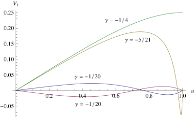
Our main results for the frequency dependence of the conductivity without self-duality are given in Fig. 1.
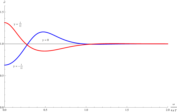
Here is the sole parameter controlling the pertinent higher derivative terms in the bulk action; we will argue that physical consistency conditions imply the constraint .
For , the frequency dependence has the same non-monotonic form as that expected by extrapolation from the weak-coupling Boltzmann analysis [6]: a collision-dominated Drude peak at small , which is then smoothly connected to the collisionless -independent conductivity at large . This similarity implies that a description of transport in terms of collisions of charged particles is a reasonable starting point for .
On the other hand, for , we observe that it is the inverse of the conductivity, i.e., the resistivity, which has a Drude-like peak at small . Under particle-vortex duality, the resistivity of the particles maps onto the conductivity of the vortices [11], as we will review here in Section 6.1. Thus, for , we conclude that a better description of charge transport is provided by considering the motion and collisions of vortices. In other words, for , it is the excitations of the dual holographic CFT, obtained under the EM duality of the bulk theory, which provide a Boltzmann-like interpretation of the frequency dependence of the conductivity.
An outline of the rest paper is as follows: In section 2, we review some basic background material, mainly to motivate the introduction of the higher derivative interaction for the gauge fields. In section 3, we calculate the charge diffusion constant and susceptibility for the dual CFT. We turn to the conductivity in section 4 and in particular, we demonstrate that in the modified theory, the conductivity is a nontrivial function of . In section 5, we derive constraints that arise on the coupling to the new gauge field interaction by imposing certain consistency conditions in the dual CFT. We examine electromagnetic duality in the modified gauge theory in section 6. We conclude with a brief discussion of our results and future directions in section 7. A discussion of the Green’s functions at finite frequency and finite momentum is presented in appendix A. In particular, we examine the relationship between the Green’s functions in the two boundary theories related by EM duality in the bulk.
2 Preliminaries
As with many of the recent excursions in the AdS/CMT, our starting point is the standard Einstein-Maxwell theory (with a negative cosmological constant) in four dimensions. Hence the action may be written as
| (1) |
The four-dimensional AdS vacuum solution of the above theory corresponds to the vacuum of the dual three-dimensional CFT. Of course, the theory also has (neutral) planar AdS black hole solutions:
| (2) |
where . In these coordinates, the asymptotic boundary is at and the event horizon, at . This solution is dual to the boundary CFT at temperature , where the temperature is given by the Hawking temperature of the black hole
| (3) |
At a certain point in the following analysis, it will also be convenient to work with a new radial coordinate: . In this coordinate system, the black hole metric becomes
| (4) |
where . Now the asymptotic boundary is at and horizon at .
As discussed in the introduction, we wish to extend the bulk theory by adding higher derivative interactions. As usual in quantum field theory, it is natural to organize the interactions by their dimension or alternatively by the number of derivatives. The Einstein-Maxwell action (1) contains all covariant terms up to two derivatives, which preserve parity, i.e., which are constructed without using the totally antisymmetric tensor. Hence it is natural to next consider the possible interactions at fourth order in derivatives [27]. In all, one can construct 15 covariant parity-conserving terms using the metric curvature, the gauge field strength and their derivatives [27]. However, using integration by parts,111Note that we also treat the four-dimensional Euler density, , as trivial since it does not effect the equations of motion. as well as the identities , the general four-derivative action can be reduced to eight independent terms
| (5) | |||||
where , and the are some unspecified coupling constants.
In a string theory context, one might expect all of these interactions to emerge in the low-energy effective action as quantum (i.e., string-loop) or corrections to the two-derivative supergravity action – see, for example, [28]. In such a context, these terms would be part of a perturbative expansion where the contribution of the higher order terms is suppressed by powers of, e.g., the ratio of the string scale over the curvature scale. From the perspective of the dual conformal gauge theory, these contributions would represent corrections suppressed by inverse powers of the ‘t Hooft coupling and/or the number of colours. Within this perturbative framework, one is also free to use field redefinitions to simplify the general bulk action (5). In the present case, field redefinitions can be used to set to zero all of the couplings except three, e.g., , and [27]. Examining the remaining three terms, the and terms involve four powers of the field strength and so would not modify the conductivity, at least if we study the latter at zero density. Hence we are left to consider only the term which couples two powers of the field strength to the spacetime curvature. The latter will certainly modify the charge transport properties of the CFT and, as we discuss in detail in section 6, it also ruins the EM self-duality of the bulk Maxwell theory.
While these string theory considerations naturally lead us to focus our attention on a single new four-derivative interaction, they are limited to the perturbative framework described above. However, we would also like to extend our analysis to the case where the new interactions are making finite modifications of the transport properties. In this case, we should think of the holographic theory as a toy model whose behaviour might be indicative of that of a complete string theory model. Recently the utility of this approach has been shown in holographic investigations with various higher curvature gravity theories – see, for example, [25, 29, 30, 31, 32]. Further, while the couplings of the higher derivative interactions are finite in this approach, consistency of the dual CFT prevents these couplings of from becoming very large, at least in simple models, as we discuss in section 5.
So given this perspective of constructing a toy model with finite couplings, let us re-examine each of the terms in the general action (5). The first two terms are curvature-squared interactions which do not involve the gauge field. Hence from the CFT perspective, these terms would only modify the -point functions of the stress tensor and so are not relevant to the charge transport. Again, the third and fourth terms involve four field strengths and so these would only modify the four-point correlator of the dual current. Hence, as noted above, these terms will again be irrelevant to the charge transport, if we limit ourselves to the case of a vanishing chemical potential. Considering next the term, we note that it contains two powers of the field strength and so will modify the charge transport. However, this term produces higher derivative equations of motion for the gauge field and so, as explained in detail in [33], the dual CFT will contain nonunitary operators. Hence we discard this term in the analysis at finite coupling to avoid this problem. Finally, the last two terms in the action (5) also involve and again modify the charge transport. However, as we discuss in more detail in section 7, they only do so in a trivial way by renormalizing the overall coefficient of the Maxwell term. Therefore we are again naturally led to consider the interaction alone in studying the transport properties of dual CFT.
Hence we will study the holographic transport properties with the following effective action for bulk Maxwell field:
| (6) |
where we have formulated the extra four-derivative interaction in terms of the Weyl tensor . That is, it is constructed as a particular linear combination of the terms in the general action (5). This particular interaction has the advantage that it leaves the charge transport at zero temperature unchanged since the Weyl curvature vanishes in the AdS geometry. Further the factor of was introduced above so that the coupling is dimensionless. From this action, we find the generalized vector equations of motion:
| (7) |
Note that the AdS vacuum and (neutral) planar black hole solution (2) are still solutions of the modified metric equations produced by the new action.
In closing this discussion, we must note that the four-derivative interaction in eq. (6) has also appeared in previous holographic studies [24, 34, 35]. In particular, [24, 34] considered the restrictions that must be imposed on the coupling in order that the dual CFT is physically consistent. While [35] focused primarily on a five-dimensional bulk theory, there is considerable overlap between the latter and the present paper. In particular, [35] considered the charge diffusion constant and (zero-frequency) conductivity, as in section 3, and bounds arising from requiring micro-causality of the dual CFT, as in section 5.
3 Diffusion Constant and Susceptibility
In this section, we calculate the charge diffusion constant and susceptibility, two quantities which control the two point Green’s function of the dual current in the limit of low frequency and long wavelength [7]. We follow [30, 35] to extend the analysis of [36] to accommodate our modified Maxwell action (6). We begin by writing a generalized action which is quadratic in the field strength:
| (8) |
where the background tensor necessarily has the following symmetries,
| (9) |
The standard Maxwell theory would be recovered by setting
| (10) |
where we can think of as the identity matrix acting in the space of two-forms (or anti-symmetric matrices). That is, given an arbitrary two-form , then . With the generalized action in eq. (8), the theory of interest (6) is constructed by setting
| (11) |
Extending the discussion of the membrane paradigm in [36] to this generalized framework is straightforward [30]. One defines the stretched horizon at (with and ) and the natural conserved current to consider is then
| (12) |
where is an outward-pointing radial unit vector. Then following the analysis in [36], one arrives at the following expression for the charge diffusion constant [30]:222As noted in [30], there are two conditions required for the following general formulae to hold. The tensor is: i) nonsingular on the horizon and ii) ‘diagonal’ in the sense discussed in section 6. Of course, in the present case, both of these requirements are satisfied by eq. (11).
| (13) |
Further applying Ohm’s law on stretched horizon, the conductivity at zero frequency is given by [35]
| (14) |
Lastly, the susceptibility is easily determined using the Einstein relation . Combining this relation with eqs. (13) and (14), an expression for is easily read off as [35]
| (15) |
Of course, if one replaces as in eq. (10), then these expressions reduce to the expected results for Einstein-Maxwell theory, e.g., see [7].
In the present case, we are interested in as given in eq. (11) where the Weyl tensor is evaluated for the planar AdS black hole (2). Hence we find
| (16) |
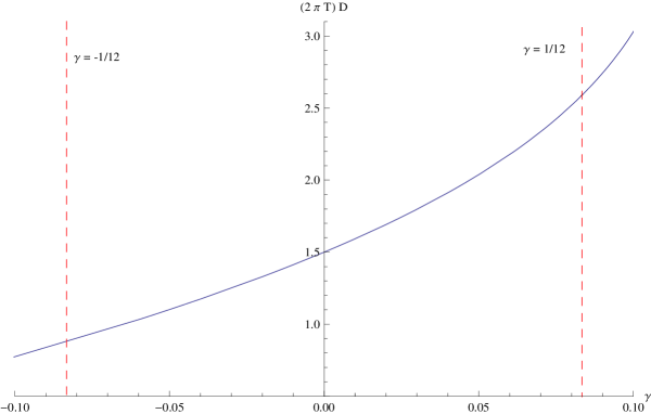
Combining these expressions in eq. (13), we find the diffusion constant to be
| (17) |
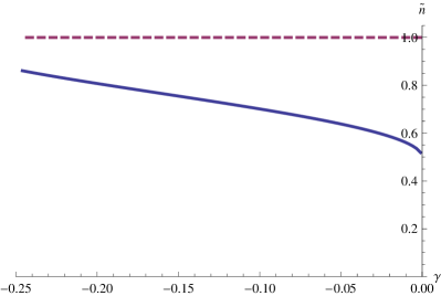
A plot of this result is given in Fig. 2. If we consider , this expression simplifies to
| (18) |
A perturbative result for to linear order in was presented in [35] for arbitrary dimensions and our results above match that for the case of a three-dimensional CFT.
Next using (14), we find
| (19) |
Note that this expression is the exact result for arbitrary . The simple -dependence appearing in the conductivity contrasts with the complicated formula for the diffusion constant (17). Of course, the diffusion constant still varies very smoothly with in the physical regime, as shown in Fig. 2. We will confirm the above result by directly evaluating the two-point function of the dual current in the next section.
Given these results and the Einstein relation , the susceptibility is easily determined to be
| (20) |
Again considering small , the susceptibility reduces to
| (21) |
4 Conductivity
In this section, we calculate the conductivity for the CFT dual to the bulk action (6). We begin by decomposing the gauge field as
| (22) |
where . For convenience and without loss of generality, we choose three-momentum vector to be . Further we choose the gauge in which . Then evaluating modified Maxwell’s equations (7) in the planar black hole background (4), we find
| (23) | |||||
| (24) | |||||
| (25) | |||||
| (26) |
Now we can use equations (23) and (24) to decouple equation of motion for :
| (27) |
where
| (28) |
At this point, recall that in the analysis of the Maxwell theory in [7], the equations of motion for and , i.e., the limit of eqs. (26) and (27), were identical. This was a result of the EM self-duality of this bulk theory. However, clearly eqs. (26) and (27) are no longer identical with nonvanishing , indicating that the new interaction in eq. (6) breaks the EM self-duality in the present case. We return to examine the EM duality in detail in section 6.
Next we solve eq. (26) with an infalling boundary condition at the horizon. Near the horizon, we can write where is regular at . Inserting this ansatz in eq. (26), we find that . The ingoing boundary condition at the horizon fixes
| (29) |
where we have defined the dimensionless frequency
| (30) |
As we wish to calculate the conductivity with but (recall that is spatial momentum along -direction), we simplify the notation by denoting and by and . With given by (29), for , the equation of motion for reduces to
| (31) | |||
To proceed further, we need to recall the relation of the conductivity to the retarded Green’s function for the dual current :
| (32) |
Of course, we wish to calculate using the AdS/CFT correspondence, following [37]. Briefly, integrating by parts in the action (6), the bulk contribution vanishes by the equations of motion (7) and so the result reduces to a surface term. At the asymptotic boundary, one has the following contribution for
| (33) | |||||
The simple expression in the second line results from explicitly evaluating the expression with the black hole metric (4) for which
| (34) |
The Fourier transform of is required to compare the above expression with the standard AdS/CFT result
| (35) |
Hence we can arrive at the usual result, i.e., the coupling makes no explicit appearance here,
| (36) |
Focusing our attention on the case and adopting the notation introduced above eq. (31), the retarded Green’s function becomes
| (37) |
Then eq. (32) yields the conductivity at as
| (38) |
Given the above expression, it is straightforward to calculate conductivity for small analytically and confirm the result (19) for derived in the previous section using the membrane paradigm. First, we make a Taylor expansion of in and substitute the ansatz into (31). Then, we find that and should satisfy the following
| (39) | ||||
| (40) |
After solving eq. (39) for , we can fix one of the integration constants demanding that is regular at the horizon. This yields , where is an arbitrary constant. Given , we solve eq. (40) for . In this case, we fix the two integration constants by imposing the following two conditions: First, is regular at the horizon. Second, we normalize such that its value at the horizon is independent of , i.e., . The final result is given by
| (41) | ||||
Now we can simply use in eq. (38), take the limit and find
| (42) |
which agrees with our previous result (14).
To study frequency dependant conductivity, we must solve eq. (31) numerically. Our numerical integrations run outward from the horizon and so we need to fix the initial conditions at . To determine the latter we solve eq. (31) for , finding
| (43) |
Numerical integration is used to determine out to the boundary at for fixed values of (and ) and then we use the complete solution and eq. (38) to calculate conductivity . In figure 1, we show our results for various values of coupling constant .
5 Bounds on the Coupling
In this section, we find the constraints that are imposed on the coupling by demanding that the dual CFT respects causality, following the analysis described in [31, 29, 35]. We also examine if there are any unstable modes of the vector field, as discussed in [38, 30], which would result in our calculations of the charge transport properties being unreliable. From a dual perspective, such unstable modes indicate that the uniform neutral plasma is an unstable configuration in the dual CFT.
To examine causality, the first step is to re-express the equations of motion of the two independent vector modes, i.e., eqs. (26) and (27), in the form of the Schrödinger equation. We begin by considering eq. (27). Recall that we are working in the gauge where and we have chosen . Now if we make a coordinate transformation to such that
| (44) |
and write where
| (45) |
then eq. (27) takes the form
| (46) |
In this Schrödinger form, the effective potential can be expressed in terms of as
| (47) |
where
| (48) | ||||
| (49) | ||||
| (50) |
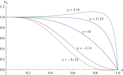
It is easiest to consider the limit , in which case one can solve for in a WKB approximation [31]. In this limit, will dominate the potential and we want to examine how its properties change as is varied, e.g., following [29]. In Fig. 3, we have plotted potential for various values of . We observe that if is too large, the potential develops a maximum with at some point between and . In that case, there will be ‘super-luminal’ modes with indicating that causality is violated in the dual CFT [31, 29]. One can easily verify that this new maximum appears for by examining the behaviour of near the boundary, i.e., near , where eq. (49) yields
| (51) |
Next we turn to the transverse vector mode satisfying eq. (26). As above, we make a change of coordinate to satisfying eq. (44) and we write where
| (52) |
With these choices, eq. (26) reduces to the desired Schrödinger form
| (53) |
where
| (54) | ||||
| (55) | ||||
| (56) |
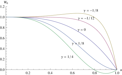
We again consider the WKB limit where dominates the potential. The shape of this potential is also shown in Fig. 3 for various values of . Examining the potential (55) as above, we find that a maximum develops for , indicating that causality is violated in the dual CFT in this regime.
Combining the results from both modes, we find that the dual CFT is only consistent (i.e., respects causality) if
| (57) |
We also note that these bounds coming from the violation of micro-causality precisely match the bounds derived for the dual parameter in the CFT derived in [24, 34]. There, various thought experiments were proposed to constrain CFT’s in four dimensions. However, their discussion is readily adapted to the three dimensions, as we consider here. The relevant experiment consists of first producing a disturbance, which is localized and injects a fixed energy, with an insertion of the current , where is a constant (spatial) polarization tensor. Then one measures the energy flux escaping to null infinity in the direction indicated by a unit vector :
| (58) |
The final result takes the form
| (59) | |||||
where is the total energy and is the angle between the direction and the polarization . The structure of this expression is completely dictated by the symmetry of the construction and the (constant) coefficient is a parameter which characterizes the underlying CFT. Given eq. (59), it is clear that is related to the parameters appearing in the general three-point correlator – see discussion in section 7. Now, the interesting observation of [24] was that if the coefficient becomes too large, the energy flux measured in various directions will become negative. Hence demanding that the energy flux should be positive in all directions for a consistent CFT leads to the constraints
| (60) |
Of course, to relate this result to that in eq. (57), we must find the relation between for our holographic CFT and the bulk coupling . The simplest approach is to use the AdS/CFT correspondence to examine the bulk dual of the thought experiment presented above. As noted above, in calculating the flux expectation value in eq. (59), we are essentially determining a specific component of the three-point function of the stress tensor with two currents. Hence in our holographic description, we must introduce an appropriate metric fluctuation and two gauge field perturbations in the AdS4 bulk, which couple to the boundary insertions of and . We then evaluate the on-shell contribution for these three insertions with the action (6). We do not present the details here, as the analogous calculations for are presented in Appendix D of [24] – the interested reader may also find the discussion in the first reference in [25] useful. In the end, the holographic calculations yield a very simple final result
| (61) |
and hence we find the bounds in eqs. (57) and (60) are equivalent.
Next we turn to possible instabilities in the neutral plasma. If we examine the potential in more detail, we find that another interesting feature develops for . That is, the potential develops a minimum at some radius close to the horizon where . The appearance of this potential well can be verified analytically by expanding near ,
| (62) |
While always vanishes at , we see that for , immediately in front of the horizon indicating the presence of the negative potential well there. In the WKB limit, this potential well leads to bound states with a negative (effective) energy, which correspond to unstable quasinormal modes in the bulk theory [38]. While these modes do not signal a fundamental pathology with the dual CFT, they do indicate that the uniform neutral plasma is unstable in this regime. Hence our calculation of the conductivity would be unreliable here. Of course, our previous constraints (57) have already ruled out as being physically interesting and so we need not worry about these instabilities.
On the other hand, one may worry that additional instabilities will appear outside of the WKB regime, considered above. In particular for small momentum, the effective potential will also receive an important contribution from . We find that for , also develops a negative minimum close to the horizon and so there might be some unstable modes in the plasma in this regime as well. We have plotted the potential for various values of the coupling constant in Fig. 4. While the WKB approximation may be less reliable in this regime, the analysis in [38] suggests that it is sufficient to determine the appearance of unstable modes. According to WKB approximation, a zero energy bound state can appear in this potential well for
| (63) |
where is a positive integer and the integration is over the values of for which the potential is negative. A plot of is given in Fig. 4. We see that reaches a maximum value of approximately 0.86, implying that the potential well is never able to support a negative energy bound state. Hence we conclude that there are no unstable modes in this low momentum regime.
While we have discussed both small and large momenta limit of our effective potential , one may still imagine that instabilities can still arise at some finite momenta. However, such a possibility can be eliminated by considering the structure of our complete potential . That is, for any finite momenta and for , the negative dip in potential is smaller than the dip in because of the positive contribution coming from . Hence there are no instabilities coming from the longitudinal vector mode in the regime (57) of physical interest.
Of course, one must also consider possible instabilities in the transverse vector mode. In this case, examining the potential , we find that a negative minimum again develops for . So again instabilities appear in the large momentum limit but only for values of the coupling outside of the physical regime (57). As above, one can also consider the low and finite momentum regimes, however, again one finds that there are no additional instabilities in the physical regime. Hence although both the transverse and longitudinal modes of the vector exhibit instabilities, these only appear in a regime where our previous constraints already indicate that the CFT is pathological.
Examining eq. (62), one sees that the potential is also negative in front of the horizon for (as well as for , as discussed above). However, this behaviour is not indicative of a negative potential well in this case. Rather a closer examination of the full potential (49) shows that a simple pole appears at , which lies in the physical interval for . The potential exhibits a similar behaviour for . The analysis and physical interpretation of the modes in this case are more elaborate along the lines of that given in [25]. However, we do not consider these issues further here since our previous constraints (57) already indicate that and are outside of the physically viable regime.
6 EM Self-Duality Lost
In this section, we examine in more detail the loss of electromagnetic (EM) self-duality for the U(1) gauge theory defined by the bulk action (6). Recall from [7] that this EM self-duality was the key property of the standard four-dimensional Maxwell theory which lead to the simple relation:
| (64) |
where and are the scalar functions determining the transverse and longitudinal components of the retarded current-current correlator – see appendix A for further discussion. As a result, the conductivity (at zero momentum) was a fixed constant for all values of . In examining the explicit equations of motion, (26) and (27), we already noted that self-duality is lost in the new theory. However, in the context of any gauge theory, one can think of EM duality as simply a change of variables in the corresponding path integral. Even if our new gauge theory (6) is not self-dual, we can still implement this change of variables and construct the EM dual theory, as we will demonstrate below.
We begin by introducing a (vector) Lagrange multiplier in the generalized action (8) as follows
| (65) |
Here is totally antisymmetric tensor, with . The fundamental fields in the path integral for this action are the two-form and the one-form . Now the EM duality comes from simply treating the integration over these fields in two different orders.
If we evaluate the path integral by first integrating over the Lagrange multiplier , the latter integration enforces the Bianchi identity on the two-form , i.e.,
| (66) |
If is to satisfy this constraint,333Note that we are justified in using ordinary (rather than covariant) derivatives both here and in the action (65) because of the antisymmetry of the indices. then on a topologically trivial background, it must take the form . Hence the remaining path integral reduces to the ‘standard’ gauge theory where the fundamental field is the Maxwell potential with generalized action given in eq. (8).
Alternatively, one can perform the path integral over the two-form first. In this case, we first integrate by parts in the second term in the action (65)
| (67) |
where we have defined the new field strength . We can now shift the original two-form field to
| (68) |
where is defined by
| (69) |
Recall the definition of given in eq. (10). With this shift, one has a trivial Gaussian integral over the field after which one is left with the path integral over the one-form with the action
| (70) |
where and
In the second equality above, the two -tensors have been eliminated with the four-dimensional identity of the form – note that the overall minus sign appears because we are working in Minkowski signature. Hence now plays the role of the gauge potential in the EM dual theory with the action (70).
The relation between the gauge fields in the two dual EM theories is implicit in the equations of motion for or . From eq. (68), we see that setting yields
| (72) |
Recall that in the usual Maxwell theory, takes the simple form given in eq. (10). In this case, and one can easily show that eq. (6) also yields . Hence for the Maxwell theory, the form of the two actions, (8) and (70), as well as the corresponding equations of motion for and , are identical. This is then a demonstration that the Maxwell theory is self-dual. Further, the duality relation between the two field strengths in eq. (72) corresponds to the usual Hodge duality, as expected for this case.
Of course, in general, we will find that and so this self-duality property is lost. That is, the form of the action and the equations of motion in the original theory and its dual now have different forms, i.e.,
| (73) |
For the action of interest (6), is given in eq. (11) and at least in a regime where we treat as small, we can write
| (74) |
Further because of the traceless property of the Weyl tensor, one finds
| (75) |
With the change in sign of the order contribution between eqs. (11) and (74), it is clear that our gauge theory is no longer self-dual.
Actually given the planar black hole background (4), it is straightforward to calculate exactly. First, we define a six-dimensional space of (antisymmetric) index pairs with, i.e., – note both the ordering of both the indices and the index pairs presented here. Then given in eq. (11) becomes a diagonal six-by-six matrix
| (76) |
where . Since is a diagonal matrix, is also a diagonal matrix whose entries are simply the inverses of those given in eq. (76). Note that takes its maximum value at the horizon , i.e., . Hence we must constrain in order for the inverse to exist everywhere in the region outside of the horizon. Of course, it is not a coincidence that the effective Schrödinger equation in section 5 became problematic (i.e., the effective potentials contained a pole) precisely outside of the same interval. In any event, the physical regime (57) for determined in section 5 lies well within this range.
Using this notation and the background metric (4), becomes the following ‘anti-diagonal’ six-by-six matrix
| (77) |
Combining these expressions, we can easily evaluate the duality transformation (72), which is expressed using the new notation as
| (78) |
The final result is
| (79) | |||||
This duality transformation gives us a precise analytic relation between the original gauge field and that, , in the EM dual theory. Of course, it would be less straightforward to express these duality relations in a covariant construction using the Weyl curvature tensor.
As discussed in [7], from the perspective of the boundary field theory, we can describe the CFT in terms of the original conserved current (dual to the bulk vector ) or a new current (dual to ). In the case of the Maxwell theory, the EM self-duality means that both currents have identical correlators. In the present case, where EM self-duality is lost, the correlators still have a simple relation which is summarized by
| (80) | |||||
The detailed derivation for these relations can be found in appendix A. The self-dual version of eq. (80), with , appeared in [7]. However, the conventions for the EM duality transformation were different there, i.e., they chose . This choice changes the normalization of the dual currents and so changes the constant on the right-hand-side of eq. (80) to . In any event, these relations imply, the longitudinal correlator in one theory is traded for the transverse correlator in the dual theory, as reflected in eq. (79). Notably, eq. (80) has precisely the same form as that obtained from general considerations of particle-vortex duality, but without self-duality, in the condensed matter context, as we review in the following subsection.
6.1 Particle-Vortex Duality
Above, we discussed EM duality as a change of variables which allows us to formulate the bulk theory in terms of two different gauge potentials. This reformulation of the bulk theory implies that the boundary CFT can be developed in terms of two ‘dual’ sets of currents, whose correlators are simply related using eq. (80). As noted in [7], the latter is reminiscent of the structure of the correlators in systems exhibiting particle-vortex duality. The discussion there focused on self-dual examples, however, the latter is an inessential feature to produce eq. (80), as we illustrate with the following simple example – see also appendix B of [7].
Consider the field theory of a complex scalar coupled to a U(1) gauge field
| (81) |
We now look at the structure of the conserved U(1) currents of , and their correlators. For simplicity, we will restrict our discussion to to make the main point in the simplest context. There is a natural generalization to , which is needed to obtain the full structure of the relationship in eq. (80), and which was discussed in [7].
The theory has the obvious conserved U(1) current
| (82) |
Because of current conservation, we can write the two-point correlator of this current in the form (reminder, we are at )
| (83) |
Here, we note that this correlator has been defined to be irreducible with respect to the propagator of the photon, .
The theory has a second conserved U(1) current; this is the ‘topological’ current
| (84) |
We can interpret as the current of dual set of particles which are the Abrikosov-Nielsen-Olesen vortices of the Abelian-Higgs model in eq (81). Each such vortex carries total flux of , and hence the prefactor above. Indeed, there is a dual formulation of the theory in eq (81) in which the vortices become the fundamental complex scalar field :
| (85) |
This dual theory has no gauge field because the vortices of only have short-range interactions. The particle number current of this dual theory is the same as that in eq. (84)
| (86) |
Now, returning to the perspective of the original theory in eq (81) and the U(1) current in eq. (84), we can write the two-point correlator of in the general form
| (87) |
where is the photon self-energy.
The photon couples linearly to the current , and so the photon self energy is clearly the irreducible correlator, and so
| (88) |
Also as in IR, we have – recall that here we are assuming the spacetime dimension . So we have
| (89) |
| (90) |
This result is clearly the analog of eq. (80). It is easily generalized to , after separation into transverse and longitudinal components, but we refrain from presenting those details here.
7 Discussion
Our main results for the frequency dependence of the conductivity without self-duality were given in Fig. 1, and we presented a physical interpretation in Section 1. For , the results had a qualitative similarity to that expected from a Boltzmann transport theory of interacting particles, while for the results resembled the Boltzmann transport of vortices.
We will now discuss other aspects of these results. We also see from Fig. 1 that the large frequency limit is unaffected by the new coupling, i.e., . We can understand this result from the fact that the Weyl curvature vanishes in the asymptotic region of the black hole region and so the new interaction in eq. (6) has no effect there.
Further, we have
| (91) |
and so this ratio varies between 4/3 and 2/3 in the allowed physical regime given in eq. (57). Thus the allowed range of variation in the conductivity by non-self-duality is smaller than 33% and can have either sign, in our model. This should be contrasted from the large variation obtained from the weak-coupling Boltzmann analyses. In the expansion (where is the spacetime dimension), it was found that generically [6]
| (92) |
Similarly, in the large expansion (where is the number of components of a vector (and not matrix) field), we have [8]
| (93) |
In both cases, the ratio becomes large in the regime of applicability of the analysis. Thus the AdS/CFT analysis gives a useful result for this ratio in the complementary limit of very strong interactions.
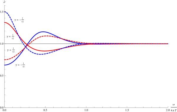
Also note that the conductivity in Fig. 1 does not vary monotonically, rather it seems there is an extremum at . For , this oscillation is as anticipated from Drude-like considerations of particle transport in ref. [6], and for we argued in Section 1 that such an oscillation is obtained from Drude-like vortex transport. Recall that in the AdS/CFT correspondence, particle-vortex duality in the boundary theory is realized as EM duality in the bulk theory. Hence we can make the previous point explicit for our holographic model using the formalism developed in Section 6. That is, for any given value of , we can explicitly construct the EM dual theory and evaluate the conductivity. In Fig. 5, we have plotted the resulting conductivities for the original bulk theory and the EM dual theory for . As expected, for , the conductivity of the dual theory exhibits a Drude-like peak at small . For , a similar peak appears for the original theory while the EM dual theory exhibits a dip in the conductivity at small . For either value of , the figure also illustrates that the conductivities of the two dual theories are not precise inverses of one another, except for . This occurs because the function is only precisely real in the latter limits.
Oscillations in the conductivity similar to those in Fig. 1 were observed in [39]. The latter studied the transport properties of currents on a three-dimensional defect immersed in the thermal path of a four-dimensional superconformal gauge theory. The holographic bulk theory consisted of probe D-branes embedded in AdS and the oscillations were an effect of stringy corrections to the usual D-brane action. Implicitly, the four-derivative interaction considered there would have been a linear combination of the terms in eq. (5). In this previous setting, the calculations were perturbative and the oscillatory contribution to the conductivity was suppressed by a factor of relative to the constant term produced by the Maxwell action on the brane – as usual, denotes the ‘t Hooft coupling of the four-dimensional gauge theory.
Section 2 provided some motivation for introducing the new four-derivative interaction in eq. (6). However, there was a certain liberty in choosing the precise form of the curvature in this interaction. From a certain perspective, the following vector action may be preferred:
| (94) |
The advantage of the higher-derivative term above is that it produces second-order equations of motion for both the gauge field and metric in any general background. We can think of this term arising from Kaluza-Klein reduction of Gauss-Bonnet gravity in five-dimensional space-time [40]. Now the generalized Maxwell’s equations are
| (95) |
Before considering the charge transport for this theory, we note that AdS vacuum and the neutral black hole (2) remain unmodified with this choice of the four-derivative interaction. In particular then, for the black-hole background, we still satisfy the vacuum Einstein equations, i.e., . Further, the Reimann curvature tensor is related to the Weyl tensor by
| (96) |
By substituting these relations into eq. (94), we find that the action becomes
| (97) |
Hence, this expression for action is identical to eq. (6) if we identify the couplings:
| (98) |
Hence in the neutral plasma, all of the charge transport properties of the new theory are identical to those found in the main text, as long as we make this identification of the couplings in the bulk gauge theory. For example, we have explicitly applied the analysis of section 5 to the new action (94) and found this produces the constraints . One can easily verify that this range precisely matches that in eq. (57) for using the identification of the gauge theory couplings in eq. (98).
It would be interesting to examine charged black holes in this new theory (94). Beyond analyzing the effects of adding a chemical potential in the boundary CFT, it would be interesting to examine the so-called “entropy problem” in this theory. That is, at zero temperature, charged black holes still have a finite horizon area for the Einstein-Maxwell theory in the bulk and hence the dual CFT has a large entropy even at but nonvanishing chemical potential. It would be interesting to determine how this feature found in simple holographic CFT’s is affected by the introduction of the new higher derivative bulk interaction in eqs. (6) or (94). Such investigations would require numerical work that would be greatly facilitated by having second-order equations, as produced by the above action (94).
As discussed in the introduction, we are following a program of expanding the universality class of the holographic CFT by introducing new higher-derivative interactions to the bulk action. The simplest way to characterize the effect of the new interactions is to examine the changes which are produced in the vacuum -point functions in the CFT. As alluded to above, the Weyl curvature vanishes in AdS space and so we may infer that in the vacuum of the dual CFT (with vanishing temperature and charge density), there are no changes to any of two-point functions, i.e., and , where the subscript 0 indicates the two-point functions are evaluated in the vacuum or at . That is, the two-point functions are independent of in the vacuum. In particular then, the charge transport properties of the holographic CFT must be independent of at . On the other hand, recall the simple dependence which appears in eq. (19) for the conductivity at . Clearly, this means that the limits, and , do not commute, as was also emphasized in ref. [6].
As described in [24, 34], the key effect of the new bulk interaction (6) is to modify the three-point correlator . One can show that in any CFT, conformal symmetry will completely fix this three-point function between the stress tensor and two conserved currents up to two constant parameters [26]. One of these parameters vanishes in the holographic dual of an Einstein-Maxwell theory. However, this extra parameter is nonvanishing for the CFT dual for our extended theory with . In particular, as discussed in section 5, the parameter in eq. (59) is only nonvanishing in the boundary CFT when . Of course in a thermal bath, the expectation value of the stress tensor is nonvanishing. Hence it should be possible to use the previous three-point function to infer the leading modification to the two-point correlator at finite temperature, e.g., with an approach similar to that considered in [41]. In principle then, such a (perturbative) calculation in the CFT should already indicate that self-duality is lost.
Above, we discussed the behavior of the conductivity, which is related to the current correlator at zero momentum. We also studied the full momentum dependence of these correlators and obtained the duality relation in eq. (80), which applied in the general case without self-duality. Remarkably, this has the same form as that obtained by applying particle-vortex duality to a (2+1)-dimensional field theory of a single complex scalar, as we reviewed in section 6.1: note that this theory is not self-dual (and self-duality is not expected in general, except for a particular theory with two complex scalar fields [7, 42]). In the single scalar field case, as discussed in section 6.1, characterize the transverse/longitudinal components of the two-point correlations of the current of the scalar particles – see eq. (103) – while characterize the corresponding quantities of the vortex current.
Of course, the constants on the right-hand-side of eqs. (80) and (90) are seen to be different. In both cases, this constant depends on the conventions used to normalize the currents and a new normalization would change the constant in either model. Hence one may ask if these relations can be expressed in a way which removes this ambiguity. As we will show, one possibility is to replace eq. (80) by
| (99) | |||||
where is the conductivity at zero momentum and zero frequency and is the same quantity for the dual currents. For our holographic model, was given in eq. (19) and given the discussion in section 6, it is a simple exercise to show that . Hence, in this case, we easily recover eq. (80) from eq. (99) above. However, the latter equation applies quite generally as we will now show: First, given the expressions for and in eqs. (32) and (105), respectively, it is straightforward to show that . Further with vanishing momentum, and hence we also have Now if we know that the product is constant, we can evaluate the constant at vanishing momentum and vanishing frequency and then our discussion leads us to write eq. (99). This expression will apply independent of the conventions used to normalize the currents and applies equally well for the field theory examples considered in section 6.1 and in [7] as for our holographic model.
The holographic relation of EM duality in the bulk and particle-vortex duality in the boundary theory was first noted in [7, 43] and the effect of this bulk transformation on the boundary transport properties was further studied in [44] – see also [39, 45]. Particle-vortex duality can be extended to an action on three-dimensional CFT’s [43, 46] and the holographic realization of these group transformations on the bulk theory was discussed in [43]. In particular, the transformation corresponds to applying EM duality in the bulk. To discuss the transformation, the bulk action must be extended to include a -term and acting with the generator corresponds to making a shift of . Of course, implicitly or explicitly, the previous holographic discussions assumed a standard Maxwell action for the bulk vector. It would be interesting to extend this discussion of the full action to the generalized action (8) introduced in section 3. Associating the generator with EM duality as in [43], one can easily verify that using eq. (72). To include the generator, we would need generalize to include parity violating terms, i.e., nonvanishing and in eq. (122). We leave this as an interesting open question.
To close, we wish to emphasize that our investigation here has considered a simple toy model and one should be circumspect in interpreting the results of our analysis. While string theory will generate the higher derivative interactions in our action (6), it certainly also produces many other higher order terms which schematically take the form . For example, some such terms, were explicitly constructed (amongst many others) and studied in [47]. Any terms with this schematic form would still fall in the class of our general action (8) and so modify the charge transport properties in a similar way. A key feature of our model was that we were able to identify physical restrictions which constrained the new coupling to fall in relatively narrow range (57). As a result, the conductivity remained relatively close to the self-dual value. Our expectation is that similar restrictions appear for general string models, however, finding more comprehensive physical constraints in this context remains an interesting open question [48]. As seen here and elsewhere [24, 29, 30, 34], the interplay between the boundary and bulk theories in the AdS/CFT correspondence is beginning to provide new insights into this question.
Acknowledgments: We thank Cliff Burgess, Jaume Gomis, Sean Hartnoll, Brandon Robinson, Brian Sheih and Aninda Sinha for discussions. SS would like to thank T. Senthil for noting the connection between vortex transport and the conductivity. AS would like to thank Jorge Escobedo, Yu-Xiang Gu and Sayeh Rajabi for fruitful and stimulating discussions. Research at Perimeter Institute is supported by the Government of Canada through Industry Canada and by the Province of Ontario through the Ministry of Research & Innovation. RCM also acknowledges support from an NSERC Discovery grant and funding from the Canadian Institute for Advanced Research. SS is grateful to the Perimeter Institute for hospitality, and acknowledges support by the National Science Foundation under grant DMR-0757145, by the FQXi foundation, and by a MURI grant from AFOSR.
Appendix A Retarded Green’s functions and EM duality
In this appendix, we find the retarded Green’s functions of currents in the boundary field theory for finite frequency and finite momentum and further we examine the relationship between the Green’s functions in the two theories related by EM duality in the bulk. In this discussion, we work with the general vector action (8) and its EM dual (70). Recall that the relation between coefficients and appearing in these two actions is given in eq. (6) and the field strengths in the two theories are given by and , respectively. Further the duality relation between these two field strengths is given in eq. (72).
For simplicity, we will begin by assuming that is diagonal in the six-dimensional space defined by the antisymmteric index pairs
| (100) |
This property holds for the specific theory (6) studied in the main text, as shown in eq. (76). We comment on more general cases at the end of the appendix. Given this assumption, we write
| (101) |
Further rotational symmetry in the -plane would restrict this ansatz with and . However, we leave this symmetry as implicit, since it is not required in the following. Now the inverse444We assume that the functions remain finite and positive throughout in order that is invertible and the bulk propagators for the gauge potential are well-behaved there. is simply the diagonal matrix with entries and, given eq. (6), is also diagonal with
| (102) | |||||
Now we review the general structure of the Green’s functions in the boundary theory, from the discussion in [7]. Together current conservation and spatial rotational invariance – Lorentz invariance is lost with – dictate the form of the retarded Green’s functions as
| (103) |
where we use the notation: , and . Further, and are orthogonal projection operators defined by
| (104) |
with denoting spatial indices while run over both space and time. If, for simplicity, we choose , then we have
| (105) |
Of course, this general structure applies for both boundary theories, that is, both for the theory dual to the vector potential and that dual to . Our notation will be that the above expressions refer to the theory dual to while , and are the corresponding expressions for the boundary currents dual to .
The first step in the holographic calculation of the Green’s functions is to solve the bulk equations of motion. Hence we begin as in section 4 by taking a plane-wave ansatz (22) for and . Further, we choose and work in radial gauge with . With these choices and the background metric (4), the equations of motion become:
| (106) | ||||
| (107) | ||||
| (108) | ||||
| (109) |
where we recall that . For the EM dual gauge theory, the equations of motion are given by simply replacing and in the expressions above.
In general, there are two independent physical modes for the four-dimensional bulk gauge field. Above, we see that decouples in eq. (109) to provide one of these modes, while and are coupled in the remaining equations. Of course, the analogous results apply to in the EM dual theory. Now explicitly writing out the duality relations (78) in the present case, we find
| (110) | |||||
Hence, at a schematic level, EM duality exchanges the mode for that in and similarly the and are exchanged. Given the holographic relationship between the bulk and boundary theories, we expect that there are connections between the Green’s functions, and , generalizing those found in [7]. However, given the previous observation, more specifically, should be related to (as well as and ) and similarly , to .
To develop these connections in detail, we must extend the holographic calculation of the Green’s functions given in section 4 to include the mixing between and , noted above. First, we solve the equations of motion (106)-(109) for with infalling boundary conditions at the horizon and asymptotic boundary conditions: . To account for mixing between different components of the gauge potential, we may write [7]: . Now, substituting the solutions into the action (8) and integrating by parts leaves an surface term at the asymptotic boundary, which generalizes that given in eq. (33),
| (111) |
After Fourier transforming in the boundary directions, we extract the desired Green’s functions as
| (112) | |||||
| (113) | |||||
| (114) | |||||
| (115) |
Here we have used that the equations of motion (106–109) only mix and . One may also easily verify that eq. (115) reduces to the expression in eq. (37) when , as in the main text.
Next consider the Green’s functions . Assume that we have where is a solution of eq. (109) satisfying the appropriate boundary conditions. In particularly, the asymptotic normalization is . Then from (115), we have
| (116) |
Given that EM duality exchanges with , we now look for a relation between this result and that for . From the expression for in eq. (110), we find and so provides a solution of the equations of motion for in the EM dual theory. While it is clear that the required infalling boundary condition is satisfied at the horizon with , we must expect that the normalization has to be adjusted in order to satisfy the desired asymptotic boundary condition. Hence we introduce a new constant setting . In order to fix this constant, we consider the analog of eq. (107) in the EM dual theory and take the limit to find
| (117) |
where deriving this expression uses and . Now the EM dual counterpart of eq. (112) yields
| (118) |
Here we have used the relations: and . Hence, combining eqs. (116) and (118), we find
| (119) |
Further, using eq. (105), this relation can be written as
| (120) |
Now it is clear that the EM dual version of the above discussion would follow through without change. That is, we would begin by constructing an expression for analogous to eq. (116) and then the counterpart of eq. (118) for . The final result emerging from these results would then be
| (121) |
To close our discussion, we comment on more general cases where contains off-diagonal terms. To begin, let us write the most general tensor which is consistent with rotational symmetry in the -plane:
| (122) |
where we are using the notation introduced in eq. (100), as well as the background metric (4). Note the pre-factors in the off-diagonal terms reflect the tensor structure of , which is slightly obscure in this notation, e.g., . Now, as noted above, rotational invariance imposes two relations on the diagonal entries, i.e., and . However, as shown above, this symmetry is remarkably restrictive on the off-diagonal components as well and our general tensor (122) only contains three independent terms amongst all of the possible entries. Now, if we further demand that this background tensor preserves parity, we must in fact set and we are left with only one function determining all of the allowed off-diagonal components. Note that these remaining off-diagonal terms preserve parity but violate time-reversal invariance.555The and terms violate both parity and time-reversal invariance.
If we restrict ourselves to the parity invariant case, it is straightforward to generalize our previous discussion to accommodate the general above (with ). Although the intermediate expressions are somewhat more involved, we find that the final Green’s functions still satisfy eqs. (120) and (121).
Note that parity invariance was implicit in the decomposition of the Green’s functions in eq. (103). If parity violating terms were allowed there would be an additional contribution of the form.
| (123) |
Hence the present analysis must be revised to accommodate these parity violating terms. Our expectation is that particle-vortex duality still provides relations between the three functions , and , describing the Green’s functions of the two dual theories. A preliminary examination of the equations of motion and the EM duality relations suggests that, in this general case, , , and their dual counterparts should satisfy three relations. However, the details of this interesting case are left as an open problem for future work.
References
- [1] J. M. Maldacena, “The large N limit of superconformal field theories and supergravity,” Adv. Theor. Math. Phys. 2, 231 (1998) [Int. J. Theor. Phys. 38, 1113 (1999)] [arXiv:hep-th/9711200].
-
[2]
S.S. Gubser, I.R. Klebanov and
A.M. Polyakov, “Gauge theory correlators from non-critical string
theory,”
Phys. Lett. B 428 (1998) 105 [arXiv:hep-th/9802109];
E. Witten, Adv. Theor. Math. Phys. 2 (1998) 253 [arXiv:hep-th/9802150]. - [3] O. Aharony, S.S. Gubser, J.M. Maldacena, H. Ooguri and Y. Oz, “Large N field theories, string theory and gravity,” Phys. Rept. 323 (2000) 183 [arXiv:hep-th/9905111].
-
[4]
See, for example:
S. A. Hartnoll, “Lectures on holographic methods for condensed matter physics,” Class. Quant. Grav. 26, 224002 (2009) [arXiv:0903.3246 [hep-th]];
C. P. Herzog, “Lectures on Holographic Superfluidity and Superconductivity,” J. Phys. A 42, 343001 (2009) [arXiv:0904.1975 [hep-th]].
S. Sachdev, “Condensed matter and AdS/CFT,” arXiv:1002.2947 [hep-th]. -
[5]
See, for example:
D. T. Son, “Toward an AdS/cold atoms correspondence: a geometric realization of the Schrödinger symmetry,” Phys. Rev. D 78 (2008) 046003 [arXiv:0804.3972 [hep-th]];
K. Balasubramanian and J. McGreevy, “Gravity duals for non-relativistic CFTs,” Phys. Rev. Lett. 101, 061601 (2008) [arXiv:0804.4053 [hep-th]];
S. Kachru, X. Liu and M. Mulligan, “Gravity Duals of Lifshitz-like Fixed Points,” Phys. Rev. D 78, 106005 (2008) [arXiv:0808.1725 [hep-th]]. - [6] K. Damle and S. Sachdev, “Non-zero temperature transport near quantum critical points,” Phys. Rev. B 56, 8714 (1997) [arXiv:cond-mat/9705206].
- [7] C. P. Herzog, P. Kovtun, S. Sachdev and D. T. Son, “Quantum critical transport, duality, and M-theory,” Phys. Rev. D 75, 085020 (2007) [arXiv:hep-th/0701036].
- [8] S. Sachdev, Quantum Phase Transitions, Cambridge University Press (1999).
- [9] P. Kovtun, D. T. Son and A. O. Starinets, “Viscosity in strongly interacting quantum field theories from black hole physics,” Phys. Rev. Lett. 94, 111601 (2005) [arXiv:hep-th/0405231].
- [10] See articles in the May 2010 issue of Physics Today.
- [11] M. P. A. Fisher, “Quantum phase transitions in disordered two-dimensional superconductors,” Phys. Rev. Lett. 65, 923 (1990).
- [12] M. Steiner, N. Breznay, and A. Kapitulnik, “Approach to a superconductor-to-Bose-insulator transition in disordered films,” Phys. Rev. B 77, 212501 (2008).
- [13] L. W. Engel, D. Shahar, C. Kurdak, and D. C. Tsui, “Microwave frequency dependence of integer quantum Hall effect: Evidence for finite-frequency scaling,” Phys. Rev. Lett. 71, 2638 (1993).
- [14] R. Crane, N. P. Armitage, A. Johansson, G. Sambandamurthy, D. Shahar, and G. Grüner, “Survival of superconducting correlations across the two-dimensional superconductor-insulator transition: A finite-frequency study,” Phys. Rev. B 75, 184530 (2007).
- [15] M. Müller, L. Fritz, and S. Sachdev, “Quantum-critical relativistic magnetotransport in graphene,” Phys. Rev. B 78, 115406 (2008) [arXiv:0805.1413 [cond-mat]].
- [16] Z. Q. Li, E. A. Henriksen, Z. Jiang, Z. Hao, M. C. Martin, P. Kim, H. L. Stormer, and D. N. Basov, “Dirac charge dynamics in graphene by infrared spectroscopy,” Nature Physics 4, 532 (2008).
- [17] Kin Fai Mak, M. Y. Sfeir, Yang Wu, Chun Hung Lui, J. A. Misewich, and T. F. Heinz, “Measurement of the Optical Conductivity of Graphene,” Phys. Rev. Lett. 101, 196405 (2008).
- [18] M. Müller, J. Schmalian, and L. Fritz, “Graphene - a nearly perfect fluid,” Phys. Rev. Lett. 103, 025301 (2009) [arXiv:0903.4178 [cond-mat]].
- [19] E. Fradkin and S. Kivelson, “Modular invariance, self-duality and the phase transition between quantum Hall plateaus,” Nucl. Phys. B 474, 543 (1996).
- [20] D. Shahar, D. C. Tsui, M. Shayegan, E. Shimshoni, and S. L. Sondhi, “Evidence for Charge-Flux Duality near the Quantum Hall Liquid-to-Insulator Transition,” Science 274, 589 (1996).
- [21] E. Shimshoni, S. L. Sondhi, and D. Shahar, “Duality near quantum Hall transitions,” Phys. Rev. B 55, 13730 (1997).
- [22] A. Bayntun, C. P. Burgess, B. P. Dolan and S. S. Lee, “AdS/QHE: Towards a Holographic Description of Quantum Hall Experiments,” arXiv:1008.1917 [hep-th].
- [23] A. Karch and S. L. Sondhi, “Non-linear, Finite Frequency Quantum Critical Transport from AdS/CFT,” arXiv:1008.4134 [cond-mat.str-el].
- [24] D. M. Hofman and J. Maldacena, “Conformal collider physics: Energy and charge correlations,” JHEP 0805, 012 (2008) [arXiv:0803.1467 [hep-th]].
-
[25]
R. C. Myers, M. F. Paulos and A. Sinha,
“Holographic studies of quasi-topological gravity,”
JHEP 1008, 035 (2010)
[arXiv:1004.2055 [hep-th]];
R. C. Myers and B. Robinson, “Black Holes in Quasi-topological Gravity,” JHEP 1008, 067 (2010) [arXiv:1003.5357 [gr-qc]]. -
[26]
H. Osborn and A. C. Petkou,
“Implications of Conformal Invariance in Field Theories for General
Dimensions,”
Annals Phys. 231, 311 (1994)
[arXiv:hep-th/9307010];
J. Erdmenger and H. Osborn, “Conserved currents and the energy-momentum tensor in conformally invariant theories for general dimensions,” Nucl. Phys. B 483, 431 (1997) [arXiv:hep-th/9605009]. - [27] R. C. Myers, M. F. Paulos and A. Sinha, “Holographic Hydrodynamics with a Chemical Potential,” JHEP 0906, 006 (2009) [arXiv:0903.2834 [hep-th]].
-
[28]
K. Hanaki, K. Ohashi and Y. Tachikawa,
“Supersymmetric Completion of an Term in Five-Dimensional
Supergravity,”
Prog. Theor. Phys. 117, 533 (2007)
[arXiv:hep-th/0611329];
S. Cremonini, K. Hanaki, J. T. Liu and P. Szepietowski, “Black holes in five-dimensional gauged supergravity with higher derivatives,” JHEP 0912, 045 (2009) [arXiv:0812.3572 [hep-th]]. - [29] A. Buchel and R. C. Myers, “Causality of Holographic Hydrodynamics,” JHEP 0908, 016 (2009) [arXiv:0906.2922 [hep-th]].
- [30] M. Brigante, H. Liu, R. C. Myers, S. Shenker and S. Yaida, “Viscosity Bound Violation in Higher Derivative Gravity,” Phys. Rev. D 77, 126006 (2008) [arXiv:0712.0805 [hep-th]].
- [31] M. Brigante, H. Liu, R. C. Myers, S. Shenker and S. Yaida, “The Viscosity Bound and Causality Violation,” Phys. Rev. Lett. 100, 191601 (2008) [arXiv:0802.3318 [hep-th]].
-
[32]
J. de Boer, M. Kulaxizi and A. Parnachev,
“AdS7/CFT6, Gauss-Bonnet Gravity, and Viscosity Bound,”
JHEP 1003, 087 (2010)
[arXiv:0910.5347 [hep-th]];
X. O. Camanho and J. D. Edelstein, “Causality constraints in AdS/CFT from conformal collider physics and Gauss-Bonnet gravity,” JHEP 1004, 007 (2010) [arXiv:0911.3160 [hep-th]];
A. Buchel, J. Escobedo, R. C. Myers, M. F. Paulos, A. Sinha and M. Smolkin, “Holographic GB gravity in arbitrary dimensions,” JHEP 1003, 111 (2010) [arXiv:0911.4257 [hep-th]];
X. H. Ge and S. J. Sin, “Shear viscosity, instability and the upper bound of the Gauss-Bonnet coupling constant,” JHEP 0905, 051 (2009) [arXiv:0903.2527 [hep-th]];
R. G. Cai, Z. Y. Nie and Y. W. Sun, “Shear Viscosity from Effective Couplings of Gravitons,” Phys. Rev. D 78, 126007 (2008) [arXiv:0811.1665 [hep-th]];
X. H. Ge, S. J. Sin, S. F. Wu and G. H. Yang, “Shear viscosity and instability from third order Lovelock gravity,” Phys. Rev. D 80, 104019 (2009) [arXiv:0905.2675 [hep-th]];
J. de Boer, M. Kulaxizi and A. Parnachev, “Holographic Lovelock Gravities and Black Holes,” JHEP 1006, 008 (2010) [arXiv:0912.1877 [hep-th]];
X. O. Camanho and J. D. Edelstein, “Causality in AdS/CFT and Lovelock theory,” JHEP 1006, 099 (2010) [arXiv:0912.1944 [hep-th]];
R. C. Myers and A. Sinha, “Seeing a c-theorem with holography,” Phys. Rev. D 82, 046006 (2010) [arXiv:1006.1263 [hep-th]]. - [33] R. C. Myers and A. Sinha, “Holographic c-theorems in arbitrary dimensions,” JHEP 1101, 125 (2011) [arXiv:1011.5819 [hep-th]].
- [34] D. M. Hofman, “Higher Derivative Gravity, Causality and Positivity of Energy in a UV complete QFT,” Nucl. Phys. B 823, 174 (2009) [arXiv:0907.1625 [hep-th]].
- [35] A. Ritz and J. Ward, “Weyl corrections to holographic conductivity,” Phys. Rev. D 79, 066003 (2009) [arXiv:0811.4195 [hep-th]].
- [36] P. Kovtun, D. T. Son and A. O. Starinets, “Holography and hydrodynamics: Diffusion on stretched horizons,” JHEP 0310, 064 (2003) [arXiv:hep-th/0309213].
- [37] D. T. Son and A. O. Starinets, “Minkowski-space correlators in AdS/CFT correspondence: Recipe and applications,” JHEP 0209, 042 (2002) [arXiv:hep-th/0205051].
- [38] R. C. Myers, A. O. Starinets and R. M. Thomson, “Holographic spectral functions and diffusion constants for fundamental matter,” JHEP 0711, 091 (2007) [arXiv:0706.0162 [hep-th]].
- [39] R. C. Myers and M. C. Wapler, “Transport Properties of Holographic Defects,” JHEP 0812, 115 (2008) [arXiv:0811.0480 [hep-th]].
- [40] R. C. Myers, B. Robinson and A. Sinha, unpublished.
- [41] M. Kulaxizi and A. Parnachev, “Energy Flux Positivity and Unitarity in CFTs,” arXiv:1007.0553 [hep-th].
- [42] O. I. Motrunich and A. Vishwanath, “Emergent photons and transitions in the O(3) sigma model with hedgehog suppression,” Phys. Rev. B 70, 075104 (2004).
- [43] E. Witten, “SL(2,Z) action on three-dimensional conformal field theories with Abelian symmetry,” arXiv:hep-th/0307041.
-
[44]
S. A. Hartnoll, P. K. Kovtun, M. Muller and S. Sachdev,
“Theory of the Nernst effect near quantum phase transitions in condensed
matter, and in dyonic black holes,”
Phys. Rev. B 76, 144502 (2007)
[arXiv:0706.3215 [cond-mat.str-el]];
S. A. Hartnoll and C. P. Herzog, “Ohm’s Law at strong coupling: S duality and the cyclotron resonance,” Phys. Rev. D 76, 106012 (2007) [arXiv:0706.3228 [hep-th]]. - [45] J. Hansen and P. Kraus, “S-duality in AdS/CFT magnetohydrodynamics,” JHEP 0910, 047 (2009) [arXiv:0907.2739 [hep-th]].
- [46] C. P. Burgess and B. P. Dolan, “Particle-vortex duality and the modular group: Applications to the quantum Hall effect and other 2-D systems,” Phys. Rev. B 63, 155309 (2001) [arXiv:hep-th/0010246].
-
[47]
I. Antoniadis, E. Gava, K. S. Narain and T. R. Taylor,
“Topological amplitudes in string theory,”
Nucl. Phys. B 413, 162 (1994)
[arXiv:hep-th/9307158];
M. Bershadsky, S. Cecotti, H. Ooguri and C. Vafa, “Kodaira-Spencer theory of gravity and exact results for quantum string amplitudes,” Commun. Math. Phys. 165, 311 (1994) [arXiv:hep-th/9309140];
I. Antoniadis and S. Hohenegger, “N=4 Topological Amplitudes and Black Hole Entropy,” Nucl. Phys. B 837, 61 (2010) [arXiv:0910.5596 [hep-th]];
I. Antoniadis, S. Hohenegger, K. S. Narain and T. R. Taylor, “Deformed Topological Partition Function and Nekrasov Backgrounds,” Nucl. Phys. B 838, 253 (2010) [arXiv:1003.2832 [hep-th]]. -
[48]
See, for example:
C. Vafa, “The string landscape and the swampland,” arXiv:hep-th/0509212;
N. Arkani-Hamed, L. Motl, A. Nicolis and C. Vafa, “The string landscape, black holes and gravity as the weakest force,” JHEP 0706, 060 (2007) [arXiv:hep-th/0601001];
A. Adams, N. Arkani-Hamed, S. Dubovsky, A. Nicolis and R. Rattazzi, “Causality, analyticity and an IR obstruction to UV completion,” JHEP 0610, 014 (2006) [arXiv:hep-th/0602178];
V. Kumar and W. Taylor, “String Universality in Six Dimensions,” arXiv:0906.0987 [hep-th];
W. Taylor, “Anomaly constraints and string/F-theory geometry in 6D quantum gravity,” arXiv:1009.1246 [hep-th].