Abstract

We present here a general approach to treat reflection and refraction of light of arbitrary polarization from single axis anisotropic plates. We show that reflection from interface inside the anisotropic medium is accompanied by beam splitting and can create surface waves.

1 Introduction

Theory of anisotropic media in optics alienates by its complexity, phenomenology and not transparent physics [1, 2, 3, 4, 5]. The most recent paper related to this field is published in Am.J.Phys.-[6] only in 1977. It is understandable that no one likes to discuss this topic. In the science of almost two hundred years old it seems hopeless to propose something new which can be attractive to students. Nevertheless, in this paper we will do just that. We will present an approach similar to that, used for description of elastic waves in anisotropic media [7]

The single axis anisotropic nonmagnetic media in electromagnetism can be described by a matrix of dielectric permittivity $\varepsilon$ with matrix elements [1]

$$\mbox{\boldmath$\varepsilon$}_{ij}=\epsilon_{0}\delta_{ij}+\epsilon^{\prime}a_{i}a_{j},$$ (1)

where $\epsilon_{0}$ is isotropical part, and anisotropy is characterized by the unit vector $a$ with components $a_{i}$ and by anisotropy parameter $\epsilon^{\prime}$. With this matrix we will first consider propagation of electromagnetic waves in a homogeneous anisotropic medium, then refraction at the interface between anisotropic and isotropic media, and after that discuss reflection and transmission of an anisotropic plain plate of finite thickness. Time to time along the text we make digression to isotropic media, because on one side it helps to check correctness of our formulas, and on the other side it is useful, because isotropic media also represent some difficulties.

Of course, some our formulas look huge, but we don’t care about it. We do not even derive some formulas and leave it to those who will need it. In fact, it is sufficient to know how to derive them, and if necessary to use a computer.

2 Waves in an anisotropic medium

The wave equation for, say, electric field $\mbox{\boldmath$E$}(\mbox{\boldmath$r$},t)$, is obtained from Maxwell equations. In a homogeneous nonmagnetic ($\mu=1$) anisotropic medium it is

$$-[\mbox{\boldmath$\nabla$}\times[\mbox{\boldmath$\nabla$}\times\mbox{\boldmath$E$}(\mbox{\boldmath$r$},t)]]=\displaystyle\frac{\partial^{2}}{c^{2}\partial t^{2}}\mbox{\boldmath$\varepsilon$}\mbox{\boldmath$E$}(\mbox{\boldmath$r$},t),$$ (2)

Solution of this equation can be accepted in the form of a plain wave

$$\mbox{\boldmath$E$}(\mbox{\boldmath$r$},t)=\mbox{\boldmath$\cal E$}\exp(i\mbox{\boldmath$k$}\cdot\mbox{\boldmath$r$}-i\omega t),$$ (3)

where $\cal E$ is a polarization vector, which can be of not unit length.

After substitution of (3) into (2) we obtain

$$k^{2}\mbox{\boldmath$\cal E$}-\mbox{\boldmath$k$}(\mbox{\boldmath$k$}\cdot\mbox{\boldmath$\cal E$})=k_{0}^{2}\mbox{\boldmath$\varepsilon$}\mbox{\boldmath$\cal E$},$$ (4)

where $k_{0}=\omega/c$, and $\varepsilon$$\cal E$, according to (1) is

$$\mbox{\boldmath$\varepsilon$}\mbox{\boldmath$\cal E$}=\epsilon_{0}\mbox{\boldmath$\cal E$}+\epsilon^{\prime}\mbox{\boldmath$a$}(\mbox{\boldmath$a$}\cdot\mbox{\boldmath$\cal E$}).$$ (5)

In isotropic media polarization vector $\cal E$ can have arbitrary direction perpendicular to the wave vector $k$. In anisotropic media it is not so.

Besides (5) the field $\mbox{\boldmath$E$}(\mbox{\boldmath$r$},t)$ should also satisfy Maxwell equation

$$\mbox{\boldmath$\nabla$}\cdot\mbox{\boldmath$\varepsilon$}\mbox{\boldmath$E$}(\mbox{\boldmath$r$},t)=0,$$ (6)

from which, after substitution of (3), it follows a limitation on possible choices of directions for $\cal E$:

$$\epsilon_{0}(\mbox{\boldmath$k$}\cdot\mbox{\boldmath$\cal E$})+\epsilon^{\prime}(\mbox{\boldmath$k$}\cdot\mbox{\boldmath$a$})(\mbox{\boldmath$a$}\cdot\mbox{\boldmath$\cal E$})=0.$$ (7)

If $k$ is not parallel to $a$, we have three independent vectors $a$, $\mbox{\boldmath$\kappa$}=\mbox{\boldmath$k$}/k$ and $\mbox{\boldmath$e$}_{1}=[\mbox{\boldmath$a$}\times\mbox{\boldmath$\kappa$}]$, which can serve a basis of a coordinate system. The basis is not orthonormal, nevertheless the vector $\cal E$ can be represented in this basis as

$$\mbox{\boldmath$\cal E$}=\alpha\mbox{\boldmath$a$}+\beta\mbox{\boldmath$\kappa$}+\gamma\mbox{\boldmath$e$}_{1}$$ (8)

with some coordinates $\alpha$, $\beta$ and $\gamma$, which are not arbitrary, as will be now shown.

Substitution of (8) into (7) gives

$$\epsilon_{0}[k\beta+(\mbox{\boldmath$k$}\cdot\mbox{\boldmath$a$})\alpha]+\epsilon^{\prime}(\mbox{\boldmath$k$}\cdot\mbox{\boldmath$a$})[\alpha+\beta(\mbox{\boldmath$\kappa$}\cdot\mbox{\boldmath$a$})]=0,$$ (9)

from which it follows that

$$\beta=-\displaystyle\frac{(\mbox{\boldmath$\kappa$}\cdot\mbox{\boldmath$a$})(1+\eta)}{1+\eta(\mbox{\boldmath$\kappa$}\cdot\mbox{\boldmath$a$})^{2}}\alpha,$$ (10)

where $\eta=\epsilon^{\prime}/\epsilon_{0}$. Substitution of (10) into (8) gives

$$\mbox{\boldmath$\cal E$}=\alpha\left(\mbox{\boldmath$a$}-\mbox{\boldmath$\kappa$}\displaystyle\frac{(\mbox{\boldmath$\kappa$}\cdot\mbox{\boldmath$a$})(1+\eta)}{1+\eta(\mbox{\boldmath$\kappa$}\cdot\mbox{\boldmath$a$})^{2}}\right)+\gamma\mbox{\boldmath$e$}_{1}=\alpha\mbox{\boldmath$e$}_{2}+\gamma\mbox{\boldmath$e$}_{1},$$ (11)

which shows that in fact we have only two independent vectors for expansion of $\cal E$: vector $\mbox{\boldmath$e$}_{1}=[\mbox{\boldmath$a$}\times\mbox{\boldmath$\kappa$}]$ orthogonal to the plane of $\mbox{\boldmath$a$},\mbox{\boldmath$k$}$, and the vector

$$\mbox{\boldmath$e$}_{2}=\mbox{\boldmath$a$}-\mbox{\boldmath$\kappa$}\displaystyle\frac{(\mbox{\boldmath$\kappa$}\cdot\mbox{\boldmath$a$})(1+\eta)}{1+\eta(\mbox{\boldmath$\kappa$}\cdot\mbox{\boldmath$a$})^{2}}.$$ (12)

It is worth to note that $\mbox{\boldmath$e$}_{2}$ is not an eigen vector of matrix $\varepsilon$, but the matrix $\varepsilon$ transforms $\mbox{\boldmath$e$}_{2}$ into a vector orthogonal to $k$

$$\mbox{\boldmath$\varepsilon$}\mbox{\boldmath$e$}_{2}=\epsilon_{1}(\theta)[\mbox{\boldmath$\kappa$}\times[\mbox{\boldmath$a$}\times\mbox{\boldmath$\kappa$}]],$$ (13)

where

$$\epsilon_{1}(\theta)=\epsilon_{0}\displaystyle\frac{1+\eta}{1+\eta(\mbox{\boldmath$\kappa$}\cdot\mbox{\boldmath$a$})^{2}}=\epsilon_{0}\displaystyle\frac{1+\eta}{1+\eta\cos^{2}\theta},$$ (14)

and $\theta$ is the angle between vectors $a$ and $k$. It is seen that, if the wave propagates along $a$, the dielectric permittivity becomes $\epsilon_{1}(0)=\epsilon_{0}$, and, if the wave propagates perpendicularly to $a$, the dielectric permittivity becomes $\epsilon_{1}(\pi/2)=\epsilon_{0}+\epsilon^{\prime}$.

With account of (14) we can represent (12) as

$$\mbox{\boldmath$e$}_{2}=\mbox{\boldmath$a$}-\mbox{\boldmath$\kappa$}(\mbox{\boldmath$\kappa$}\cdot\mbox{\boldmath$a$})\epsilon_{1}(\theta)/\epsilon_{0}.$$ (15)

In the limit $\eta\to 0$, when the medium becomes isotropic we obtain

$$\lim_{\eta\to 0}\mbox{\boldmath$e$}_{2}=[\mbox{\boldmath$\kappa$}\times[\mbox{\boldmath$a$}\times\mbox{\boldmath$\kappa$}]].$$ (16)

Now we will show that in general a plain wave in anisotropic media can have polarizations only along $\mbox{\boldmath$e$}_{2}$ or $\mbox{\boldmath$e$}_{1}$.

Indeed, substitution of (11) into (4) with account of (13) gives

$$k^{2}[\alpha\mbox{\boldmath$e$}_{2}+\gamma\mbox{\boldmath$e$}_{1}-\alpha\mbox{\boldmath$\kappa$}(\mbox{\boldmath$\kappa$}\cdot\mbox{\boldmath$e$}_{2})]=k_{0}^{2}\Big{(}\alpha\epsilon_{1}(\theta)[\mbox{\boldmath$\kappa$}\times[\mbox{\boldmath$a$}\times\mbox{\boldmath$\kappa$}]]+\gamma\epsilon_{0}\mbox{\boldmath$e$}_{1}\Big{)}.$$ (17)

Multiplying it with $\mbox{\boldmath$e$}_{1}$ we obtain

$$(k^{2}-k_{0}^{2}\epsilon_{0})\gamma\mbox{\boldmath$e$}_{1}^{2}=0.$$ (18)

Therefore, if $\gamma\neq 0$, (18) can be satisfied only, when

$$k^{2}=k_{0}^{2}\epsilon_{0}.$$ (19)

Multiplying (17) with $\mbox{\boldmath$e$}_{2}$ we obtain

$$\left(k^{2}-k_{0}^{2}\epsilon_{1}(\theta)\right)\alpha[1-(\mbox{\boldmath$a$}\cdot\mbox{\boldmath$\kappa$})^{2}]=0.$$ (20)

Therefore, if $\alpha\neq 0$, and $\mbox{\boldmath$a$}\neq\mbox{\boldmath$\kappa$}$, (20) can be satisfied only, when

$$k^{2}=k_{0}^{2}\epsilon_{1}(\theta),$$ (21)

where $\epsilon_{1}(\theta)$ is given in (14). Since the length of $k$ is different for two polarization vectors, therefore a single plain wave can exist only with a single polarization along either $\mbox{\boldmath$e$}_{2}$ or $\mbox{\boldmath$e$}_{1}$.

We will call “transverse” the mode with polarization $\mbox{\boldmath$\cal E$}_{1}=\mbox{\boldmath$e$}_{1}$, and “mixed” the mode with polarization along $\mbox{\boldmath$\cal E$}_{2}=\mbox{\boldmath$e$}_{2}$. The mixed mode contains a longitudinal component – a component along the wave vector $k$. We think that such a nomenclature is better than common names: “ordinary” for $\mbox{\boldmath$\cal E$}_{1}=\mbox{\boldmath$e$}_{1}$, and “extraordinary” for $\mbox{\boldmath$\cal E$}_{2}=\mbox{\boldmath$e$}_{2}$, because our names point to physical peculiarities of these waves.

2.1 Magnetic fields

Every electromagnetic wave besides electric contains also magnetic field. For simplicity we assume that $\mu=1$. From the equation $\mbox{\boldmath$\nabla$}\cdot\mbox{\boldmath$H$}=0$, which is equivalent to $\mbox{\boldmath$k$}\cdot\mbox{\boldmath$H$}=0$, it follows that the field $H$ is orthogonal to $k$. It is also orthogonal to $\cal E$, which follows from the Maxwell equation

$$-[\mbox{\boldmath$\nabla$}\times\mbox{\boldmath$E$}(\mbox{\boldmath$r$},t)]=\frac{\partial}{c\partial t}\mbox{\boldmath$H$}(\mbox{\boldmath$r$},t).$$ (22)

After substitution of (3) and

$$\mbox{\boldmath$H$}(\mbox{\boldmath$r$},t)=\mbox{\boldmath$\cal H$}\exp(i\mbox{\boldmath$k$}\cdot\mbox{\boldmath$r$}-i\omega t),$$ (23)

with polarization vector $\cal H$ of the field $H$, we obtain

$$\mbox{\boldmath$\cal H$}=\displaystyle\frac{k}{k_{0}}[\mbox{\boldmath$\kappa$}\times\mbox{\boldmath$\cal E$}],$$ (24)

where $k_{0}=\omega/c$, and $\mbox{\boldmath$\kappa$}=\mbox{\boldmath$k$}/k$ is a unit vector along the wave vector $k$. For transverse and mixed modes, respectively, we therefore obtain

$$\mbox{\boldmath$\cal H$}_{1}=\displaystyle\frac{k}{k_{0}}[\mbox{\boldmath$\kappa$}\times\mbox{\boldmath$e$}_{1}]=\displaystyle\frac{k}{k_{0}}[\mbox{\boldmath$\kappa$}\times[\mbox{\boldmath$a$}\times\mbox{\boldmath$\kappa$}]],\qquad\mbox{\boldmath$\cal H$}_{2}=\displaystyle\frac{k}{k_{0}}[\mbox{\boldmath$\kappa$}\times\mbox{\boldmath$e$}_{2}]=\displaystyle\frac{k}{k_{0}}[\mbox{\boldmath$\kappa$}\times\mbox{\boldmath$a$}],$$ (25)

and the total plain wave field looks

$$\Psi(\mbox{\boldmath$r$},t)=\psi_{j}\exp(i\mbox{\boldmath$k$}_{j}\cdot\mbox{\boldmath$r$}-i\omega t),$$ (26)

where $\psi_{j}=\mbox{\boldmath$\cal E$}_{j}+\mbox{\boldmath$\cal H$}_{j}$, and $j$ denotes mode 1 or 2. In isotropic media we also can choose, say $\mbox{\boldmath$\cal E$}=[\mbox{\boldmath$a$}\times\mbox{\boldmath$\kappa$}]$ and $\mbox{\boldmath$\cal H$}=[\mbox{\boldmath$\kappa$}\times[\mbox{\boldmath$a$}\times\mbox{\boldmath$\kappa$}]]$. However, there $a$ can have arbitrary direction, therefore the couple of orthogonal vectors $\cal E$ and $\cal H$ can be rotated any angle around the wave vector $k$.

3 Reflection from an interface with an isotropic medium

Imagine that our space is split into two half spaces. The part at $z<0$ is an anisotropic medium, and the part at $z>0$ is vacuum with $\epsilon_{0}=1$, $\eta=0$. We have two different wave equations in these parts, and waves go from reign of one equation into reign of another one through the interface where they must obey boundary conditions imposed by Maxwell equations.

Let’s look for reflection of the two possible modes incident onto the interface within the anisotropic medium.

3.1 Nonspecularity and mode transformation at the interface

First we note that reflection of mixed mode is not specular. Indeed, since direction of $k$ after reflection changes, therefore the angle $\theta$ between $a$ and $\kappa$ does also change, and $k$, according to (21), changes too. However the component $\mbox{\boldmath$k$}_{\|}$ parallel to the interface does not change, so the change of $k$ means the change of the normal component $k_{\bot}$, and this leads to nonspecularity of the reflection.

Let’s calculate the change of $k_{\bot}$ for the incident mixed mode with wave vector $\mbox{\boldmath$k$}_{2r}$, where the index r means that the mode 2 propagates to the right toward the interface. For a given angle $\theta$ between $\mbox{\boldmath$k$}_{2r}$ and $a$ we can write

$$k_{2r\bot}=\sqrt{\displaystyle\frac{\epsilon_{0}k_{0}^{2}(1+\eta)}{1+\eta\cos^{2}\theta}-k_{\|}^{2}},$$ (27)

however the value of $k_{2r\bot}$ enters implicitly into $\cos\theta$, so to find explicit dependence of $k_{2r\bot}$ on $a$ it is necessary to solve the equation

$$k_{\|}^{2}+x^{2}+\eta(k_{\|}(\mbox{\boldmath$l$}\cdot\mbox{\boldmath$a$})+x(\mbox{\boldmath$n$}\cdot\mbox{\boldmath$a$}))^{2}=k_{0}^{2}\epsilon_{0}(1+\eta),$$ (28)

where $x$ denotes $k_{2r\bot}$, $n$ is a unit vector of normal, directed toward isotropic medium, and $l$ is a unit vector along $\mbox{\boldmath$k$}_{\|}$, which together with $n$ constitutes the plane of incidence. Solution of this equation is

$$x=\displaystyle\frac{-\eta k_{\|}(\mbox{\boldmath$n$}\cdot\mbox{\boldmath$a$})(\mbox{\boldmath$l$}\cdot\mbox{\boldmath$a$})+\sqrt{\epsilon_{0}k_{0}^{2}(1+\eta)(1+\eta(\mbox{\boldmath$n$}\cdot\mbox{\boldmath$a$})^{2})-k_{\|}^{2}(1+\eta(\mbox{\boldmath$l$}\cdot\mbox{\boldmath$a$})^{2}+\eta(\mbox{\boldmath$n$}\cdot\mbox{\boldmath$a$})^{2})}}{1+\eta(\mbox{\boldmath$n$}\cdot\mbox{\boldmath$a$})^{2}}.$$ (29)

The sign chosen before square root provides the correct asymptotics at $\eta=0$ equal to isotropic value $\sqrt{\epsilon_{0}k_{0}^{2}-k_{\|}^{2}}$.

In general vector $a$ is representable as $\mbox{\boldmath$a$}=\alpha\mbox{\boldmath$n$}+\beta\mbox{\boldmath$l$}+\gamma\mbox{\boldmath$t$}$, where $\mbox{\boldmath$t$}=[\mbox{\boldmath$n$}\mbox{\boldmath$l$}]$ is a unit vector perpendicular to the plane of incidence. The normal component $k_{2r\bot}$ depends only on part of this vector $\mbox{\boldmath$a$}^{\prime}=\alpha\mbox{\boldmath$n$}+\beta\mbox{\boldmath$l$}$, which lies in the incidence plane. If we denote $\alpha=|\mbox{\boldmath$a$}^{\prime}|\cos(\theta_{a})$, $\beta=|\mbox{\boldmath$a$}^{\prime}|\sin(\theta_{a})$, where $|\mbox{\boldmath$a$}^{\prime}|$ is projection of $a$ on the incidence plane, and introduce new parameter $\eta^{\prime}=\eta|\mbox{\boldmath$a$}^{\prime}|^{2}\leq\eta$, then formula (29) is simplified to

$$k_{2r\bot}=\displaystyle\frac{-\eta^{\prime}k_{\|}\sin(2\theta_{a})+2\sqrt{\epsilon_{0}k_{0}^{2}(1+\eta)[1+\eta^{\prime}\cos^{2}(\theta_{a})]-k_{\|}^{2}(1+\eta^{\prime})}}{2[1+\eta^{\prime}\cos^{2}(\theta_{a})]}.$$ (30)

For the reflected mixed mode (mode 2, propagating to the left from the interface) an equation similar to (28) looks

$$k_{\|}^{2}+x^{2}+\eta(k_{\|}(\mbox{\boldmath$l$}\cdot\mbox{\boldmath$a$})-x(\mbox{\boldmath$n$}\cdot\mbox{\boldmath$a$}))^{2}=k_{0}^{2}\epsilon_{0}(1+\eta),$$ (31)

where $x=k_{2l\bot}$, and its solution is

$$k_{2l\bot}=\displaystyle\frac{\eta^{\prime}k_{\|}\sin(2\theta_{a})+2\sqrt{\epsilon_{0}k_{0}^{2}(1+\eta)[1+\eta^{\prime}\cos^{2}(\theta_{a})]-k_{\|}^{2}(1+\eta^{\prime})}}{2[1+\eta^{\prime}\cos^{2}(\theta_{a})]}.$$ (32)

We see that the difference of the normal components of reflected and incident waves of mixed modes $k_{2l\bot}-k_{2r\bot}$ is

$$k_{2l\bot}-k_{2r\bot}=\displaystyle\frac{\eta^{\prime}k_{\|}\sin(2\theta_{a})}{1+\eta^{\prime}\cos^{2}(\theta_{a})},$$ (33)

In the following we will present such differences in dimensionless variables

$$\Delta_{22}\equiv\displaystyle\frac{k_{2l\bot}-k_{2r\bot}}{k_{0}\sqrt{\epsilon_{0}}}=\displaystyle\frac{\eta^{\prime}q\sin(2\theta_{a})+2\sqrt{(1+\eta)[1+\eta^{\prime}\cos^{2}(\theta_{a})]-q^{2}(1+\eta^{\prime})}}{2[1+\eta^{\prime}\cos^{2}(\theta_{a})]},$$ (34)

where $q^{2}=k_{\|}^{2}/k_{0}^{2}\epsilon_{0}$. The reflection angle depends on orientation of anisotropy vector $a$ and it can be both larger than the specular one, when $\theta_{a}>0$, or smaller, when $\theta_{a}<0$.

In the case of transverse incident mode the length $k=|\mbox{\boldmath$k$}|$ of the wave vector, according to (19), does not depend on orientation of $a$, therefore this wave is reflected specularly.

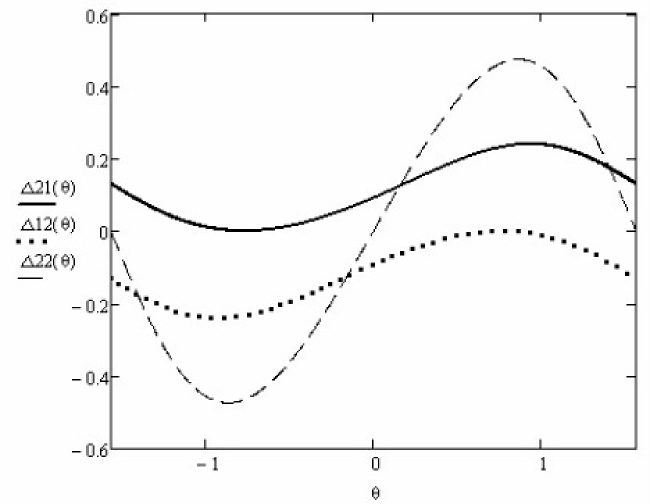
Figure 1: Variation of change $\Delta$ of normal components for reflected and incident waves in dependence of angle $\theta=\theta_{a}$ of anisotropy vector with respect to normal $n$. Vector $a$ is supposed to lie completely in the incidence plane. The curves $\Delta ij$ represent dimensionless ratio $\Delta_{ij}(\theta)$ given by (34), (35) and (36). The curves were calculated for $\eta=\eta^{\prime}=0.4$ and $q=k_{\|}/k_{0}\sqrt{\epsilon_{0}}=0.7$.

Every incident mode after reflection creates another one, without another mode it is impossible to satisfy the boundary conditions. Let’s look what will be the normal component of the other mode. If the incident is of mode 2, reflected transverse mode (mode 1 propagating to the left, away from the interface) will have $k_{1l\bot}=\sqrt{\epsilon_{0}k_{0}^{2}-k_{\|}^{2}}$. Therefore according to (30) the difference $\Delta_{12}=(k_{1l\bot}-k_{2r\bot})/k_{0}\sqrt{\epsilon_{0}}$ is

$$\Delta_{12}=\sqrt{1-q^{2}}-\displaystyle\frac{-\eta^{\prime}q\sin(2\theta_{a})+2\sqrt{(1+\eta)[1+\eta^{\prime}\cos^{2}(\theta_{a})]-q^{2}(1+\eta^{\prime})}}{2[1+\eta^{\prime}\cos^{2}(\theta_{a})]}.$$ (35)

In the opposite case, when the incident mode is transverse one, the reflected mixed mode will have $k_{2l\bot}$ shown in (32). Therefore the difference $\Delta_{21}=(k_{2l\bot}-k_{1r\bot})/k_{0}\sqrt{\epsilon_{0}}$ is

$$\Delta_{21}=\displaystyle\frac{\eta^{\prime}q\sin(2\theta_{a})+2\sqrt{(1+\eta)[1+\eta^{\prime}\cos^{2}(\theta_{a})]-q^{2}(1+\eta^{\prime})}}{2[1+\eta^{\prime}\cos^{2}(\theta_{a})]}-\sqrt{1-q^{2}}.$$ (36)

The changes of normal components with variation of $\theta_{a}$ according to (34), (35) and (36) for some values of dimensionless parameters $\eta$ and $q$ and vector $a$ lying completely in the incidence plane, are shown in Fig. 1. From this figure it is seen that the strongest deviation of reflected wave from specular direction is observed for reflection of mixed to mixed mode.

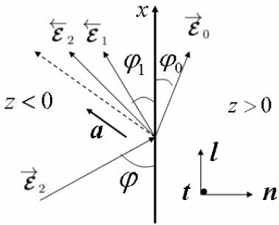
Figure 2: Arrangement of wave vectors of all the modes resulted when the incident wave is of mode 2, $\overrightarrow{\mbox{\boldmath$\cal E$}}$, and when the anisotropy vector $a$ has the direction as shown here. The grazing angle of the reflected mode 2, $\overleftarrow{\mbox{\boldmath$\cal E$}}_{2}$, is less than specular one (specular direction is shown by broken arrow), and the grazing angle $\varphi_{1}$ of the reflected mode 1, $\overleftarrow{\mbox{\boldmath$\cal E$}}_{1}$, is even lower. The grazing angle $\varphi_{0}$ of the transmitted wave $\overrightarrow{\mbox{\boldmath$\cal E$}}_{0}$ is even lower than $\varphi_{1}$. We can imagine than at some critical value $\varphi=\varphi_{c1}$ the angle $\varphi_{0}$ becomes zero. It means that at $\varphi<\varphi_{c1}$ transmitted wave becomes evanescent and all the incident energy is totally reflected in the form of two modes. More over, there exists a second critical angle $\varphi_{c2}$, when $\varphi_{1}=0$. It means that at $\varphi<\varphi_{c2}$ the mode $\overleftarrow{\mbox{\boldmath$\cal E$}}_{1}$ also becomes evanescent. In this case all the incident energy is totally reflected nonspecularly in the form of mode 2. At the same time the two evanescent waves $\overrightarrow{\mbox{\boldmath$\cal E$}}_{0}$ and $\overleftarrow{\mbox{\boldmath$\cal E$}}_{2}$ combine into a surface wave, propagating along the interface. The arrows over $\cal E$ show direction of waves propagation with respect to the interface. In the figure there is also shown the basis which is used along the paper. It consists of unit normal vector $n$ along normal ($z$-axis), unit tangential vector $l$ ($x$-axis) which together with $n$ defines the incidence plane, and the vector $t$ ($y$-axis) looking toward the reader, which is normal to the incidence plane.

Since reflection of mode 2 is in general nonspecular, it can happen that the wave vectors of reflected and transmitted waves will be arranged as shown in fig. 2, and it follows that there are two critical angles for $\varphi$. The first critical angle $\varphi_{c1}$ ($q^{2}=1/\epsilon_{0}$) is the angle of total reflection. At it the transmitted wave becomes evanescent. The totally reflected field contains two modes. At the second critical angle $\varphi_{c2}$, when $q$ is in the range

$$1<q^{2}<\displaystyle\frac{(1+\eta)(1+\eta^{\prime}cos^{2}(\theta_{a}))}{1+\eta^{\prime}}.$$ (37)

the reflected mode 1 also becomes evanescent. Together with evanescent transmitted wave the mode 1 constitutes a surface wave, propagating along the interface. In that case we have nonspecular total reflection of the mode $\mbox{\boldmath$\cal E$}_{2}$.

In figure 3 it is shown how do the normal components of wave vectors change with increase of $q$, which is equivalent to decrease of $\varphi$. For $\epsilon_{0}=1.6$ the first critical angle corresponds to $q\approx 0.8$. The second critical angle corresponds to $q=1$.

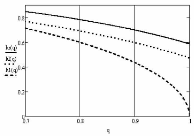
Figure 3: Dependence of dimensionless normal components of incident and reflected waves on $q=k\cos\varphi/k_{0}\sqrt{\epsilon_{0}}$. The solid curve corresponds to the incident wave moving to the right $kr(q)=k_{2r\bot}/k_{0}\sqrt{\epsilon_{0}}$. The dotted curve corresponds to the reflected wave of mode 2 moving to the left $kl(q)=k_{2l\bot}/k_{0}\sqrt{\epsilon_{0}}$. And the broken curve corresponds to the reflected wave of mode 1 moving to the left $k1(q)=k_{1l\bot}/k_{0}\sqrt{\epsilon_{0}}$. It is seen that at $q>1$ the mode 1 ceases to propagate. Its normal component $k1(q)=\sqrt{1-q^{2}}=-i\sqrt{q^{2}-1}$ becomes imaginary, therefore the reflected mode 1 becomes an evanescent wave. Together with transmitted wave, which becomes evanescent at $q^{2}=1/\epsilon_{0}$, the mode 1 constitute the surface electromagnetic wave.

3.2 Reflection and refraction from inside anisotropic medium

The wave function in the full space is

$$\Psi(\mbox{\boldmath$r$})=\Theta(z<0)\left(e^{i\overrightarrow{\mbox{\scriptsize\boldmath$k$}}_{j}\cdot\mbox{\scriptsize\boldmath$r$}}\overrightarrow{\psi}_{j}+\sum\limits_{j^{\prime}=1,2}e^{i\overleftarrow{\mbox{\scriptsize\boldmath$k$}}_{j^{\prime}}\cdot\mbox{\scriptsize\boldmath$r$}}\overleftarrow{\psi}_{j^{\prime}}\overrightarrow{\rho}_{j^{\prime}j}\right)+\Theta(z>0)e^{i\mbox{\scriptsize\boldmath$k$}_{0}\cdot\mbox{\scriptsize\boldmath$r$}}\Big{(}\psi_{e}\overrightarrow{\tau}_{ej}+\psi_{m}\overrightarrow{\tau}_{mj}\Big{)},$$ (38)

where $\psi=\mbox{\boldmath$\cal E$}+\mbox{\boldmath$\cal H$}$, arrows show direction of waves propagation, $\overrightarrow{\psi}_{j}$ denotes the incident wave of mode $j$ ($j=1,2$), $\overleftarrow{\psi}_{j^{\prime}}$ ($l=1,2$) denotes reflected wave of mode $j^{\prime}$, $\overrightarrow{\mbox{\boldmath$k$}}_{j}=(\mbox{\boldmath$k$}_{\|},k_{jr\bot})$, $\overleftarrow{\mbox{\boldmath$k$}}_{j^{\prime}}=(\mbox{\boldmath$k$}_{\|},-k_{j^{\prime}l\bot})$, $\mbox{\boldmath$k$}_{0}=(\mbox{\boldmath$k$}_{\|},\sqrt{k_{0}^{2}-k_{\|}^{2}})$, $\psi_{e,m}$, $\overrightarrow{\tau}_{e,mj}$ are fields and transmission amplitudes of TE- and TM-modes for incident $j$-mode respectively. To find reflection $\overrightarrow{\rho}$ and transmission $\overrightarrow{\tau}$ amplitudes (the arrow over them shows the direction of propagation of the incident wave toward the interface), we need to impose on (38) the following boundary conditions.

3.3 General equations from boundary conditions

Every incident wave field can be decomposed at the interface into TE- and TM-modes. In TE-mode electric field is perpendicular to the incidence plane, $\mbox{\boldmath$\cal E$}\propto\mbox{\boldmath$t$}$, therefore contribution of $j$-th mode into TE-mode is $(\mbox{\boldmath$\cal E$}_{j}\cdot\mbox{\boldmath$t$})$. In TM-mode magnetic field is perpendicular to the incidence plane, $\mbox{\boldmath$\cal H$}\propto\mbox{\boldmath$t$}$, therefore contribution of $j$-th mode into TM-mode is $(\mbox{\boldmath$\cal H$}_{j}\cdot\mbox{\boldmath$t$})$. For transmitted field in TE-mode we accept $\overrightarrow{\mbox{\boldmath$\cal E$}}_{e}=\mbox{\boldmath$t$}$, $\overrightarrow{\mbox{\boldmath$\cal H$}}_{e}=[\mbox{\boldmath$\kappa$}_{0}\times\mbox{\boldmath$t$}]$, and for transmitted field in TM-mode we accept $\overrightarrow{\mbox{\boldmath$\cal E$}}_{m}=\mbox{\boldmath$t$}$, $\overrightarrow{\mbox{\boldmath$\cal E$}}_{m}=-[\mbox{\boldmath$\kappa$}_{0}\times\mbox{\boldmath$t$}]$.

3.3.1 TE-boundary conditions

In TE-mode for incident j-mode we have the following three equations from boundary conditions:

1. continuity of electric field

   $$(\mbox{\boldmath$t$}\cdot\overrightarrow{\mbox{\boldmath$\cal E$}}_{j})+(\mbox{\boldmath$t$}\cdot\overleftarrow{\mbox{\boldmath$\cal E$}}_{1})\overrightarrow{\rho}_{1j}+(\mbox{\boldmath$t$}\cdot\overleftarrow{\mbox{\boldmath$\cal E$}}_{2})\overrightarrow{\rho}_{2j}=\overrightarrow{\tau}_{ej},$$ (39)

2. continuity of magnetic field parallel to the interface

   $$(\mbox{\boldmath$l$}\cdot\overrightarrow{\mbox{\boldmath$\cal H$}}_{j})+(\mbox{\boldmath$l$}\cdot\overleftarrow{\mbox{\boldmath$\cal H$}}_{1})\overrightarrow{\rho}_{1j}+(\mbox{\boldmath$l$}\cdot\overleftarrow{\mbox{\boldmath$\cal H$}}_{2})\overrightarrow{\rho}_{2j}=(\mbox{\boldmath$l$}\cdot[\mbox{\boldmath$\kappa$}_{0}\times\mbox{\boldmath$t$}])\overrightarrow{\tau}_{ej}\equiv-\kappa_{0\bot}\overrightarrow{\tau}_{e1},$$ (40)

3. and continuity of the normal component of magnetic induction, which for $\mu=1$ looks

   $$(\mbox{\boldmath$n$}\cdot\overrightarrow{\mbox{\boldmath$\cal H$}}_{j})+(\mbox{\boldmath$n$}\cdot\overleftarrow{\mbox{\boldmath$\cal H$}}_{1})\overrightarrow{\rho}_{1j}+(\mbox{\boldmath$n$}\cdot\overleftarrow{\mbox{\boldmath$\cal H$}}_{2})\overrightarrow{\rho}_{2j}=(\mbox{\boldmath$n$}\cdot[\mbox{\boldmath$\kappa$}_{0}\times\mbox{\boldmath$t$}])\overrightarrow{\tau}_{ej}\equiv\kappa_{0\|}\tau_{ej}.$$ (41)

The last eq. (41) is, in fact, not needed, because it coincides with (39). It is a good exercise to check the identity of (39) and (41) using explicit expressions for $\cal E$ and $\cal H$. Some examples of such substitutions will be presented in the Appendix A.

3.3.2 TM-boundary conditions

In TM-mode we have the equations

1. continuity of magnetic field

   $$(\mbox{\boldmath$t$}\cdot\overrightarrow{\mbox{\boldmath$\cal H$}}_{j})+(\mbox{\boldmath$t$}\cdot\overleftarrow{\mbox{\boldmath$\cal H$}}_{1})\overrightarrow{\rho}_{1j}+(\mbox{\boldmath$t$}\cdot\overleftarrow{\mbox{\boldmath$\cal H$}}_{2})\overrightarrow{\rho}_{2j}=\overrightarrow{\tau}_{mj},$$ (42)

2. continuity of electric field parallel to the interface

   $$(\mbox{\boldmath$l$}\cdot\overrightarrow{\mbox{\boldmath$\cal E$}}_{j})+(\mbox{\boldmath$l$}\cdot\overleftarrow{\mbox{\boldmath$\cal E$}}_{1})\overrightarrow{\rho}_{1j}+(\mbox{\boldmath$l$}\cdot\overleftarrow{\mbox{\boldmath$\cal E$}}_{2})\overrightarrow{\rho}_{2j}=-(\mbox{\boldmath$l$}\cdot[\mbox{\boldmath$\kappa$}_{0}\times\mbox{\boldmath$t$}])\overrightarrow{\tau}_{mj}\equiv\kappa_{0\bot}\overrightarrow{\tau}_{mj},$$ (43)

3. and continuity of the normal component of field $D$

   $$(\mbox{\boldmath$n$}\cdot\mbox{\boldmath$\varepsilon$}\overrightarrow{\mbox{\boldmath$\cal E$}}_{j})+(\mbox{\boldmath$n$}\cdot\mbox{\boldmath$\varepsilon$}\overleftarrow{\mbox{\boldmath$\cal E$}}_{1})\overrightarrow{\rho}_{1j}+(\mbox{\boldmath$n$}\cdot\mbox{\boldmath$\varepsilon$}\overleftarrow{\mbox{\boldmath$\cal E$}}_{2})\overrightarrow{\rho}_{2j}=-(\mbox{\boldmath$n$}\cdot[\mbox{\boldmath$\kappa$}_{0}\times\mbox{\boldmath$t$}])\overrightarrow{\tau}_{mj}\equiv\kappa_{0\|}\overrightarrow{\tau}_{mj}.$$ (44)

Again we can neglect Eq. (44), because it coincides with (42), and again it is a good, though a little bit more difficult, exercise to check identity of these equations using explicit expressions for $\cal E$ and $\cal H$. In the following we will not show third equations like b23a and (44), because they are useless.

Exclusion of $\overrightarrow{\tau}_{ej}$ from (39) and (40), and exclusion of $\overrightarrow{\tau}_{mj}$ from (42) and (43) give two equations for $\overrightarrow{\rho}_{1j}$, $\overrightarrow{\rho}_{2j}$, which is convenient to represent in the matrix form

$$\left(\begin{array}[]{cc}\left((\mbox{\boldmath$l$}\cdot\overleftarrow{\mbox{\boldmath$\cal H$}}_{1})+\kappa_{0\bot}(\mbox{\boldmath$t$}\cdot\overleftarrow{\mbox{\boldmath$\cal E$}}_{1})\right)&\left((\mbox{\boldmath$l$}\cdot\overleftarrow{\mbox{\boldmath$\cal H$}}_{2})+\kappa_{0\bot}(\mbox{\boldmath$t$}\cdot\overleftarrow{\mbox{\boldmath$\cal E$}}_{2})\right)\\ \left(\kappa_{0\bot}(\mbox{\boldmath$t$}\cdot\overleftarrow{\mbox{\boldmath$\cal H$}}_{1})-(\mbox{\boldmath$l$}\cdot\overleftarrow{\mbox{\boldmath$\cal E$}}_{1})\right)&\left(\kappa_{0\bot}(\mbox{\boldmath$t$}\cdot\overleftarrow{\mbox{\boldmath$\cal H$}}_{2})-(\mbox{\boldmath$l$}\cdot\overleftarrow{\mbox{\boldmath$\cal E$}}_{2})\right)\\ \end{array}\right){\overrightarrow{\rho}_{1j}\choose\overrightarrow{\rho}_{2j}}=-{(\mbox{\boldmath$l$}\cdot\overrightarrow{\mbox{\boldmath$\cal H$}}_{1})+\kappa_{0\bot}(\mbox{\boldmath$t$}\cdot\overrightarrow{\mbox{\boldmath$\cal E$}}_{1})\choose\kappa_{0\bot}(\mbox{\boldmath$t$}\cdot\overrightarrow{\mbox{\boldmath$\cal H$}}_{j})-(\mbox{\boldmath$l$}\cdot\overrightarrow{\mbox{\boldmath$\cal E$}}_{j})}.$$ (45)

Solution of this equation is very simple if to take into account that reciprocal of an arbitrary 2x2 matrix looks

$$\left(\begin{array}[]{cc}a&b\\ c&d\\ \end{array}\right)^{-1}=\displaystyle\frac{1}{ad-bc}\left(\begin{array}[]{cc}d&-b\\ -c&a\\ \end{array}\right).$$ (46)

Therefore

$${\overrightarrow{\rho}_{1j}\choose\overrightarrow{\rho}_{2j}}=\displaystyle\frac{1}{D}\left(\begin{array}[]{cc}-\left(\kappa_{0\bot}(\mbox{\boldmath$t$}\cdot\overleftarrow{\mbox{\boldmath$\cal H$}}_{2})-(\mbox{\boldmath$l$}\cdot\overleftarrow{\mbox{\boldmath$\cal E$}}_{2})\right)&\left((\mbox{\boldmath$l$}\cdot\overleftarrow{\mbox{\boldmath$\cal H$}}_{2})+\kappa_{0\bot}(\mbox{\boldmath$t$}\cdot\overleftarrow{\mbox{\boldmath$\cal E$}}_{2})\right)\\ \left(\kappa_{0\bot}(\mbox{\boldmath$t$}\cdot\overleftarrow{\mbox{\boldmath$\cal H$}}_{1})-(\mbox{\boldmath$l$}\cdot\overleftarrow{\mbox{\boldmath$\cal E$}}_{1})\right)&-\left((\mbox{\boldmath$l$}\cdot\overleftarrow{\mbox{\boldmath$\cal H$}}_{1})+\kappa_{0\bot}(\mbox{\boldmath$t$}\cdot\overleftarrow{\mbox{\boldmath$\cal E$}}_{1})\right)\\ \end{array}\right){(\mbox{\boldmath$l$}\cdot\overrightarrow{\mbox{\boldmath$\cal H$}}_{j})+\kappa_{0\bot}(\mbox{\boldmath$t$}\cdot\overrightarrow{\mbox{\boldmath$\cal E$}}_{j})\choose\kappa_{0\bot}(\mbox{\boldmath$t$}\cdot\overrightarrow{\mbox{\boldmath$\cal H$}}_{j})-(\mbox{\boldmath$l$}\cdot\overrightarrow{\mbox{\boldmath$\cal E$}}_{j})},$$ (47)

Where $D$ is determinant

$$D=\left((\mbox{\boldmath$l$}\cdot\overleftarrow{\mbox{\boldmath$\cal H$}}_{1})+\kappa_{0\bot}(\mbox{\boldmath$t$}\cdot\overleftarrow{\mbox{\boldmath$\cal E$}}_{1})\right)\left(\kappa_{0\bot}(\mbox{\boldmath$t$}\cdot\overleftarrow{\mbox{\boldmath$\cal H$}}_{2})-(\mbox{\boldmath$l$}\cdot\overleftarrow{\mbox{\boldmath$\cal E$}}_{2})\right)-$$

$$-\left((\mbox{\boldmath$l$}\cdot\overleftarrow{\mbox{\boldmath$\cal H$}}_{2})+\kappa_{0\bot}(\mbox{\boldmath$t$}\cdot\overleftarrow{\mbox{\boldmath$\cal E$}}_{2})\right)\left(\kappa_{0\bot}(\mbox{\boldmath$t$}\cdot\overleftarrow{\mbox{\boldmath$\cal H$}}_{1})-(\mbox{\boldmath$l$}\cdot\overleftarrow{\mbox{\boldmath$\cal E$}}_{1})\right).$$ (48)

Substitution of these expressions into (39) and (42) gives transmissions $\overrightarrow{\tau}_{e,mj}$

$${\overrightarrow{\tau}_{ej}\choose\overrightarrow{\tau}_{mj}}={(\mbox{\boldmath$t$}\cdot\overrightarrow{\mbox{\boldmath$\cal E$}}_{j})\choose(\mbox{\boldmath$t$}\cdot\overrightarrow{\mbox{\boldmath$\cal H$}}_{j})}+\left(\begin{array}[]{cc}(\mbox{\boldmath$t$}\cdot\overleftarrow{\mbox{\boldmath$\cal E$}}_{1})&(\mbox{\boldmath$t$}\cdot\overleftarrow{\mbox{\boldmath$\cal E$}}_{2})\\ (\mbox{\boldmath$t$}\cdot\overleftarrow{\mbox{\boldmath$\cal H$}}_{1})&(\mbox{\boldmath$t$}\cdot\overleftarrow{\mbox{\boldmath$\cal H$}}_{2})\\ \end{array}\right){\overrightarrow{\rho}_{1j}\choose\overrightarrow{\rho}_{2j}},$$ (49)

3.3.3 The most general case

Above we considered the case when the incident wave has polarization vector $\mbox{\boldmath$e$}_{j}$ with unit amplitude. (We remind that vectors $\mbox{\boldmath$e$}_{j}$ are not normalized to unity.) To find later reflections from plain plates we will need a more general case, when the incident wave has both modes with amplitudes $x_{1,2}$. To find amplitudes of reflected and transmitted waves in the general case it is convenient to represent the state of the incident wave in the form of 2 dimensional vector

$$|\overrightarrow{x}\rangle={\overrightarrow{x}_{1}\choose\overrightarrow{x}_{2}}.$$ (50)

then the states of reflected and transmitted waves are also described by 2-dimensional vectors, which can be represented as

$$|\overleftarrow{\psi}\rangle={\overleftarrow{\psi}_{1}\choose\overleftarrow{\psi}_{2}}=\overrightarrow{\mbox{\boldmath$\hat{\cal R}$}}^{\prime}|\overrightarrow{x}\rangle,\qquad|\overrightarrow{\psi}_{0}\rangle={\overrightarrow{\psi}_{e}\choose\overrightarrow{\psi}_{m}}=\overrightarrow{\mbox{\boldmath$\hat{\cal T}$}}^{\prime}|\overrightarrow{x}\rangle,$$ (51)

where $\overrightarrow{\mbox{\boldmath$\hat{\cal R}$}}^{\prime}$ and $\overrightarrow{\mbox{\boldmath$\hat{\cal T}$}}^{\prime}$ are two dimensional matrices

$$\overrightarrow{\mbox{\boldmath$\hat{\cal R}$}}^{\prime}=\left(\begin{array}[]{cc}\overrightarrow{\rho}_{11}&\overrightarrow{\rho}_{12}\\ \overrightarrow{\rho}_{21}&\overrightarrow{\rho}_{22}\\ \end{array}\right),\qquad\overrightarrow{\mbox{\boldmath$\hat{\cal T}$}}^{\prime}=\left(\begin{array}[]{cc}\overrightarrow{\tau}_{e1}&\overrightarrow{\tau}_{e2}\\ \overrightarrow{\tau}_{m1}&\overrightarrow{\tau}_{m2}\\ \end{array}\right).$$ (52)

We introduced the prime here and below to distinguish transmission and reflection from inside the medium from the similar matrices obtained for incident waves outside the medium.

These formulas will be used later for calculation of reflection and transmission of plain parallel anisotropic plates. In the case of a plate we have two interfaces, therefore we need also reflection and transmission at the left interface from inside and outside the plate. Reflection and transmission from inside the plate can be easily found from symmetry considerations. Their representation is obtained from (47) — (49) by reverse of arrows and change of the sign before $\kappa_{0\bot}$. After this action we find

$$\overleftarrow{\mbox{\boldmath$\hat{\cal R}$}}^{\prime}=\left(\begin{array}[]{cc}\overleftarrow{\rho}_{11}&\overleftarrow{\rho}_{12}\\ \overleftarrow{\rho}_{21}&\overleftarrow{\rho}_{22}\\ \end{array}\right),\qquad\overleftarrow{\mbox{\boldmath$\hat{\cal T}$}}^{\prime}=\left(\begin{array}[]{cc}\overleftarrow{\tau}_{e1}&\overleftarrow{\tau}_{e2}\\ \overleftarrow{\tau}_{m1}&\overleftarrow{\tau}_{m2}\\ \end{array}\right).$$ (53)

Reflection from outside the medium is to be considered separately.

3.3.4 Energy conservation

It is always necessary to control correctness of the obtained formulas. One of the best controls is the test of energy conservation. One should always check whether the energy density flux of incident wave along the normal to interface is equal to the sum of energy density fluxes of reflected and transmitted waves, and the most important in such tests is the correct definition of the energy fluxes. In isotropic media it is possible to define energy flux along a vector $n$ as

$$(\mbox{\boldmath$J$}\cdot\mbox{\boldmath$n$})=\displaystyle\frac{(\mbox{\boldmath$k$}\cdot\mbox{\boldmath$n$})}{k}\displaystyle\frac{c}{\sqrt{\epsilon}}\displaystyle\frac{\varepsilon\mbox{\boldmath$\cal E$}^{2}+\mbox{\boldmath$\cal H$}^{2}}{8\pi},$$ (54)

or

$$(\mbox{\boldmath$J$}\cdot\mbox{\boldmath$n$})=c\displaystyle\frac{(\mbox{\boldmath$n$}\cdot[\mbox{\boldmath$\cal E$}\times\mbox{\boldmath$\cal H$}])}{4\pi}.$$ (55)

In isotropic media both definitions are equivalent, because $\mbox{\boldmath$\cal H$}=[\mbox{\boldmath$k$}\times\mbox{\boldmath$\cal E$}]$, and $(\mbox{\boldmath$k$}\cdot\mbox{\boldmath$\cal E$})=0$. The first definition looks even more preferable since the second one can be written even for stationary fields, where there are no energy flux.

In anisotropic media only the second definition is valid, and because in mode 2 the field $\cal E$ is not orthogonal to $k$, the direction of the energy density flux is determined not only by wave vector, but also by direction of the field $\cal E$ itself.

3.4 Reflection and refraction from outside an anisotropic medium

Let’s consider the case, when the half space at $z<0$ is vacuum, and that at $z>0$ is an anisotropic medium. The incident wave falls onto interface from vacuum. The wave function in the full space can be represented as

$$\Psi(\mbox{\boldmath$r$})=\Theta(z<0)\Big{(}e^{i\overrightarrow{\mbox{\scriptsize\boldmath$k$}}_{0}\mbox{\scriptsize\boldmath$r$}}\overrightarrow{\psi}_{j}+e^{i\overleftarrow{\mbox{\scriptsize\boldmath$k$}}_{0}\mbox{\scriptsize\boldmath$r$}}\sum_{j^{\prime}=e,m}\overleftarrow{\psi}_{j^{\prime}}\overrightarrow{\rho}_{j^{\prime}j}\Big{)}+\Theta(z>0)\left(e^{i\overrightarrow{\mbox{\scriptsize\boldmath$k$}}_{1}\mbox{\scriptsize\boldmath$r$}}\overrightarrow{\psi}_{1}\overrightarrow{\tau}_{1j}+e^{i\overrightarrow{\mbox{\scriptsize\boldmath$k$}}_{2}\mbox{\scriptsize\boldmath$r$}}\overrightarrow{\psi}_{2}\overrightarrow{\tau}_{2j}\right),$$ (56)

where $j,j^{\prime}$ denote $e$ or $m$ for TE- and TM-modes respectively, the term $\exp(i\overrightarrow{\mbox{\boldmath$k$}}_{0}\mbox{\boldmath$r$})\overrightarrow{\mbox{\boldmath$\psi$}}_{j}$ with the wave vector $\overrightarrow{\mbox{\boldmath$k$}}_{0}=(\mbox{\boldmath$k$}_{\|},k_{0\bot}=\sqrt{k_{0}^{2}-k_{\|}^{2}})$ describes the plain wave incident on the interface from vacuum. In TE-mode factor $\overrightarrow{\mbox{\boldmath$\psi$}}_{e}=\overrightarrow{\mbox{\boldmath$\cal E$}}_{e}+\overrightarrow{\mbox{\boldmath$\cal H$}}_{e}$ contains $\overrightarrow{\mbox{\boldmath$\cal E$}}_{e}=\mbox{\boldmath$t$}$ and $\overrightarrow{\mbox{\boldmath$\cal H$}}_{e}=[\overrightarrow{\mbox{\boldmath$\kappa$}}_{0}\mbox{\boldmath$t$}]$. In TM-mode factor $\overrightarrow{\mbox{\boldmath$\psi$}}_{m}=\overrightarrow{\mbox{\boldmath$\cal E$}}_{m}+\overrightarrow{\mbox{\boldmath$\cal H$}}_{m}$ contains $\overrightarrow{\mbox{\boldmath$\cal H$}}_{e}=\mbox{\boldmath$t$}$ and $\overrightarrow{\mbox{\boldmath$\cal E$}}_{e}=-[\overrightarrow{\mbox{\boldmath$\kappa$}}_{0}\mbox{\boldmath$t$}]$.

The reflected wave has the wave vector $\overleftarrow{\mbox{\boldmath$k$}}_{0}=(\mbox{\boldmath$k$}_{\|},-k_{0\bot})$, and fields $\overleftarrow{\mbox{\boldmath$\cal E$}}_{e}=\mbox{\boldmath$t$}$, $\overleftarrow{\mbox{\boldmath$\cal H$}}_{e}=[\overleftarrow{\mbox{\boldmath$\kappa$}}_{0}\mbox{\boldmath$t$}]$, $\overleftarrow{\mbox{\boldmath$\cal H$}}_{m}=\mbox{\boldmath$t$}$, and $\overleftarrow{\mbox{\boldmath$\cal E$}}_{m}=-[\overleftarrow{\mbox{\boldmath$\kappa$}}_{0}\mbox{\boldmath$t$}]$. The refracted field contains two wave modes with wave vectors $\overrightarrow{\mbox{\boldmath$k$}}_{1}=(\mbox{\boldmath$k$}_{\|},k_{1\bot})$, $\overrightarrow{\mbox{\boldmath$k$}}_{2}=(\mbox{\boldmath$k$}_{\|},k_{2r\bot})$ and electric fields $\overrightarrow{\mbox{\boldmath$\cal E$}}_{1}=\mbox{\boldmath$e$}_{1}=[\mbox{\boldmath$a$}\overrightarrow{\mbox{\boldmath$\kappa$}}_{1}]$ and $\overrightarrow{\mbox{\boldmath$\cal E$}}_{2}=\mbox{\boldmath$e$}_{2}=\mbox{\boldmath$a$}-\overrightarrow{\mbox{\boldmath$\kappa$}}_{2}(\mbox{\boldmath$a$}\overrightarrow{\mbox{\boldmath$\kappa$}}_{2})\epsilon(\theta_{\overrightarrow{2}})/\epsilon_{0}$. Here $\mbox{\boldmath$\kappa$}=\mbox{\boldmath$k$}/k$, $k_{1\bot}=\sqrt{\epsilon_{0}k_{0}^{2}-k_{\|}^{2}}$, and $k_{\overrightarrow{2}\bot}$ is given by (30). For incident TE-mode reflection $\rho_{ee}$, $\rho_{me}$ and refraction $\tau_{je}$ amplitudes ($j=1,2$) are found from boundary conditions

$$(\mbox{\boldmath$t$}\overrightarrow{\mbox{\boldmath$\cal E$}}_{1})\overrightarrow{\tau}_{1e}+(\mbox{\boldmath$t$}\overrightarrow{\mbox{\boldmath$\cal E$}}_{2})\overrightarrow{\tau}_{2e}=1+\overrightarrow{\rho}_{ee},$$ (57)

$$(\mbox{\boldmath$l$}\overrightarrow{\mbox{\boldmath$\cal H$}}_{1})\overrightarrow{\tau}_{1e}+(\mbox{\boldmath$l$}\overrightarrow{\mbox{\boldmath$\cal H$}}_{2})\overrightarrow{\tau}_{2e}=-\kappa_{0\bot}(1-\overrightarrow{\rho}_{ee}),$$ (58)

$$(\mbox{\boldmath$t$}\overrightarrow{\mbox{\boldmath$\cal H$}}_{1})\overrightarrow{\tau}_{1e}+(\mbox{\boldmath$t$}\overrightarrow{\mbox{\boldmath$\cal H$}}_{2})\overrightarrow{\tau}_{2e}=\overrightarrow{\rho}_{me},$$ (59)

$$(\mbox{\boldmath$l$}\overrightarrow{\mbox{\boldmath$\cal E$}}_{1})\overrightarrow{\tau}_{1e}+(\mbox{\boldmath$l$}\overrightarrow{\mbox{\boldmath$\cal E$}}_{2})\overrightarrow{\tau}_{2e}=-\kappa_{0\bot}\overrightarrow{\rho}_{me}.$$ (60)

Exclusion of $\overrightarrow{\rho}_{ee}$ and $\overrightarrow{\rho}_{me}$ leads to

$$\left(\begin{array}[]{cc}\left(\kappa_{0\bot}(\mbox{\boldmath$t$}\overrightarrow{\mbox{\boldmath$\cal E$}}_{1})-(\mbox{\boldmath$l$}\overrightarrow{\mbox{\boldmath$\cal H$}}_{1})\right)&\left(\kappa_{0\bot}(\mbox{\boldmath$t$}\overrightarrow{\mbox{\boldmath$\cal E$}}_{2})-(\mbox{\boldmath$l$}\overrightarrow{\mbox{\boldmath$\cal H$}}_{2})\right)\\ \left(\kappa_{0\bot}(\mbox{\boldmath$t$}\overrightarrow{\mbox{\boldmath$\cal H$}}_{1})+(\mbox{\boldmath$l$}\overrightarrow{\mbox{\boldmath$\cal E$}}_{1})\right)&\left(\kappa_{0\bot}(\mbox{\boldmath$t$}\overrightarrow{\mbox{\boldmath$\cal H$}}_{2})+(\mbox{\boldmath$l$}\overrightarrow{\mbox{\boldmath$\cal E$}}_{2})\right)\\ \end{array}\right){\overrightarrow{\tau}_{1e}\choose\overrightarrow{\tau}_{2e}}={2\kappa_{0\bot}\choose 0}$$ (61)

and the solution

$${\overrightarrow{\tau}_{1e}\choose\overrightarrow{\tau}_{2e}}=\displaystyle\frac{1}{D_{e}}\left(\begin{array}[]{cc}\left(\kappa_{0\bot}(\mbox{\boldmath$t$}\overrightarrow{\mbox{\boldmath$\cal H$}}_{2})+(\mbox{\boldmath$l$}\overrightarrow{\mbox{\boldmath$\cal E$}}_{2})\right)&-\left(\kappa_{0\bot}(\mbox{\boldmath$t$}\overrightarrow{\mbox{\boldmath$\cal E$}}_{2})-(\mbox{\boldmath$l$}\overrightarrow{\mbox{\boldmath$\cal H$}}_{2})\right)\\ -\left(\kappa_{0\bot}(\mbox{\boldmath$t$}\overrightarrow{\mbox{\boldmath$\cal H$}}_{1})+(\mbox{\boldmath$l$}\overrightarrow{\mbox{\boldmath$\cal E$}}_{1})\right)&\left(\kappa_{0\bot}(\mbox{\boldmath$t$}\overrightarrow{\mbox{\boldmath$\cal E$}}_{1})-(\mbox{\boldmath$l$}\overrightarrow{\mbox{\boldmath$\cal H$}}_{1})\right)\\ \end{array}\right){2\kappa_{0\bot}\choose 0}$$ (62)

where $D_{e}$ is determinant

$$D_{e}=\left(\kappa_{0\bot}(\mbox{\boldmath$t$}\overrightarrow{\mbox{\boldmath$\cal E$}}_{1})-(\mbox{\boldmath$l$}\overrightarrow{\mbox{\boldmath$\cal H$}}_{1})\right)\left(\kappa_{0\bot}(\mbox{\boldmath$t$}\overrightarrow{\mbox{\boldmath$\cal H$}}_{2})+(\mbox{\boldmath$l$}\overrightarrow{\mbox{\boldmath$\cal E$}}_{2})\right)-$$

$$-\left(\kappa_{0\bot}(\mbox{\boldmath$t$}\overrightarrow{\mbox{\boldmath$\cal E$}}_{2})-(\mbox{\boldmath$l$}\overrightarrow{\mbox{\boldmath$\cal H$}}_{2})\right)\left(\kappa_{0\bot}(\mbox{\boldmath$t$}\overrightarrow{\mbox{\boldmath$\cal H$}}_{1})+(\mbox{\boldmath$l$}\overrightarrow{\mbox{\boldmath$\cal E$}}_{1})\right).$$ (63)

Substitution of $\overrightarrow{\tau}_{je}$ into (57) and (59) gives

$${\overrightarrow{\rho}_{ee}\choose\overrightarrow{\rho}_{me}}=\left(\begin{array}[]{cc}(\mbox{\boldmath$t$}\overrightarrow{\mbox{\boldmath$\cal E$}}_{1})&(\mbox{\boldmath$t$}\overrightarrow{\mbox{\boldmath$\cal E$}}_{2})\\ (\mbox{\boldmath$t$}\overrightarrow{\mbox{\boldmath$\cal H$}}_{1})&(\mbox{\boldmath$t$}\overrightarrow{\mbox{\boldmath$\cal H$}}_{2})\\ \end{array}\right){\overrightarrow{\tau}_{1e}\choose\overrightarrow{\tau}_{2e}}-{1\choose 0}.$$ (64)

In the case of incident TM-mode we have boundary conditions

$$(\mbox{\boldmath$t$}\overrightarrow{\mbox{\boldmath$\cal H$}}_{1})\overrightarrow{\tau}_{1m}+(\mbox{\boldmath$t$}\overrightarrow{\mbox{\boldmath$\cal H$}}_{2})\overrightarrow{\tau}_{2m}=1+\overrightarrow{\rho}_{mm},$$ (65)

$$(\mbox{\boldmath$l$}\overrightarrow{\mbox{\boldmath$\cal E$}}_{1})\overrightarrow{\tau}_{1m}+(\mbox{\boldmath$l$}\overrightarrow{\mbox{\boldmath$\cal E$}}_{2})\overrightarrow{\tau}_{2m}=\kappa_{0\bot}(1-\overrightarrow{\rho}_{mm}),$$ (66)

$$(\mbox{\boldmath$t$}\overrightarrow{\mbox{\boldmath$\cal E$}}_{1})\overrightarrow{\tau}_{1m}+(\mbox{\boldmath$t$}\overrightarrow{\mbox{\boldmath$\cal E$}}_{2})\overrightarrow{\tau}_{2m}=\overrightarrow{\rho}_{em},$$ (67)

$$(\mbox{\boldmath$l$}\overrightarrow{\mbox{\boldmath$\cal H$}}_{1})\overrightarrow{\tau}_{1m}+(\mbox{\boldmath$l$}\overrightarrow{\mbox{\boldmath$\cal H$}}_{2})\overrightarrow{\tau}_{2m}=\kappa_{0\bot}\overrightarrow{\rho}_{em}.$$ (68)

Exclusion of $\overrightarrow{\rho}_{me}$ and $\overrightarrow{\rho}_{mm}$ leads to

$$\left(\begin{array}[]{cc}\left(\kappa_{0\bot}(\mbox{\boldmath$t$}\overrightarrow{\mbox{\boldmath$\cal H$}}_{1})+(\mbox{\boldmath$l$}\overrightarrow{\mbox{\boldmath$\cal E$}}_{1})\right)&\left(\kappa_{0\bot}(\mbox{\boldmath$t$}\overrightarrow{\mbox{\boldmath$\cal H$}}_{2})+(\mbox{\boldmath$l$}\overrightarrow{\mbox{\boldmath$\cal E$}}_{2})\right)\\ \left(\kappa_{0\bot}(\mbox{\boldmath$t$}\overrightarrow{\mbox{\boldmath$\cal E$}}_{1})-(\mbox{\boldmath$l$}\overrightarrow{\mbox{\boldmath$\cal H$}}_{1})\right)&\left(\kappa_{0\bot}(\mbox{\boldmath$t$}\overrightarrow{\mbox{\boldmath$\cal E$}}_{2})-(\mbox{\boldmath$l$}\overrightarrow{\mbox{\boldmath$\cal H$}}_{2})\right)\\ \end{array}\right){\overrightarrow{\tau}_{1m}\choose\overrightarrow{\tau}_{2m}}={2\kappa_{0\bot}\choose 0}.$$ (69)

Therefore

$${\overrightarrow{\tau}_{1m}\choose\overrightarrow{\tau}_{2m}}=\displaystyle\frac{1}{D_{m}}\left(\begin{array}[]{cc}\left(\kappa_{0\bot}(\mbox{\boldmath$t$}\overrightarrow{\mbox{\boldmath$\cal E$}}_{2})-(\mbox{\boldmath$l$}\overrightarrow{\mbox{\boldmath$\cal H$}}_{2})\right)&-\left(\kappa_{0\bot}(\mbox{\boldmath$t$}\overrightarrow{\mbox{\boldmath$\cal H$}}_{2})+(\mbox{\boldmath$l$}\overrightarrow{\mbox{\boldmath$\cal E$}}_{2})\right)\\ -\left(\kappa_{0\bot}(\mbox{\boldmath$t$}\overrightarrow{\mbox{\boldmath$\cal E$}}_{1})-(\mbox{\boldmath$l$}\overrightarrow{\mbox{\boldmath$\cal H$}}_{1})\right)&\left(\kappa_{0\bot}(\mbox{\boldmath$t$}\overrightarrow{\mbox{\boldmath$\cal H$}}_{1})+(\mbox{\boldmath$l$}\overrightarrow{\mbox{\boldmath$\cal E$}}_{1})\right)\\ \end{array}\right){2\kappa_{0\bot}\choose 0},$$ (70)

where $D_{m}=-D_{e}$ (63). Substitution of $\overrightarrow{\tau}_{jm}$ into (65) and (67) gives

$${\overrightarrow{\rho}_{em}\choose\overrightarrow{\rho}_{mm}}=\left(\begin{array}[]{cc}(\mbox{\boldmath$t$}\overrightarrow{\mbox{\boldmath$\cal E$}}_{1})&(\mbox{\boldmath$t$}\overrightarrow{\mbox{\boldmath$\cal E$}}_{2})\\ (\mbox{\boldmath$t$}\overrightarrow{\mbox{\boldmath$\cal H$}}_{1})&(\mbox{\boldmath$t$}\overrightarrow{\mbox{\boldmath$\cal H$}}_{2})\\ \end{array}\right){\overrightarrow{\tau}_{1m}\choose\overrightarrow{\tau}_{2m}}-{0\choose 1}.$$ (71)

In the general case, when the incident wave has an amplitude $\overrightarrow{\xi}_{e}$ in TE-mode and amplitude $\overrightarrow{\xi}_{m}$ in TM-mode, the state of the incident wave can be described by two-dimensional vector

$$|\overrightarrow{\xi}_{0}\rangle={\overrightarrow{\xi}_{e}\choose\overrightarrow{\xi}_{m}},$$ (72)

and the states of reflected and transmitted waves can be represented as

$$|\overleftarrow{\xi}_{0}\rangle={\overleftarrow{\xi}_{e}\choose\overleftarrow{\xi}_{m}}=\overrightarrow{\mbox{\boldmath$\hat{\cal R}$}}|\overrightarrow{\xi}_{0}\rangle,\qquad|\overrightarrow{\xi}\rangle={\overrightarrow{\xi}_{1}\choose\overrightarrow{\xi}_{2}}=\overrightarrow{\mbox{\boldmath$\hat{\cal T}$}}|\overrightarrow{\xi}_{0}\rangle,$$ (73)

where $\overrightarrow{\mbox{\boldmath$\hat{\cal R}$}}$ and $\overrightarrow{\mbox{\boldmath$\hat{\cal T}$}}$ are the two dimensional matrices

$$\overrightarrow{\mbox{\boldmath$\hat{\cal R}$}}=\left(\begin{array}[]{cc}\overrightarrow{\rho}_{ee}&\overrightarrow{\rho}_{em}\\ \overrightarrow{\rho}_{me}&\overrightarrow{\rho}_{mm}\\ \end{array}\right),\qquad\overrightarrow{\mbox{\boldmath$\hat{\cal T}$}}=\left(\begin{array}[]{cc}\overrightarrow{\tau}_{1e}&\overrightarrow{\tau}_{1m}\\ \overrightarrow{\tau}_{2e}&\overrightarrow{\tau}_{2m}\\ \end{array}\right).$$ (74)

4 Reflection and transmission of a plain parallel plate of thickness $L$

Now, when we understand what happens at interfaces, we can construct [8] expressions for reflection, $\overrightarrow{\mbox{\boldmath$\hat{R}$}}(L)$, and transmission, $\overrightarrow{\mbox{\boldmath$\hat{T}$}}(L)$, matrices for a whole anisotropic plain parallel plate of some thickness $L$, when the state of the incident wave is described by a general vector $\overrightarrow{\xi}_{0}\rangle$. To do that let’s denote the state of field of the modes $\mbox{\boldmath$e$}_{1}$ and $\mbox{\boldmath$e$}_{2}$ incident from inside the plate onto the second interface at $z=L$ by unknown 2-dimensional vector $|\overrightarrow{x}\rangle$ (50). If we were able to find $|x\rangle$ we could immediately write the state of transmitted field

$$\overrightarrow{\mbox{\boldmath$\hat{T}$}}(L)|\overrightarrow{\xi}_{0}\rangle=\overrightarrow{\mbox{\boldmath$\hat{\cal T}$}}^{\prime}|\overrightarrow{x}\rangle,$$ (75)

and the state of the field, reflected from the whole plate

$$\overrightarrow{\mbox{\boldmath$\hat{R}$}}(L)|\overrightarrow{\xi}_{0}\rangle=\overrightarrow{\mbox{\boldmath$\hat{\cal R}$}}|\xi_{0}\rangle+\overleftarrow{\mbox{\boldmath$\hat{\cal T}$}}^{\prime}\overleftarrow{\mbox{\boldmath$\hat{E}$}}(L)\overrightarrow{\mbox{\boldmath$\hat{\cal R}$}}^{\prime}|\overrightarrow{x}\rangle,$$ (76)

where $\overleftarrow{\mbox{\boldmath$\hat{E}$}}(L)$, $\overrightarrow{\mbox{\boldmath$\hat{E}$}}(L)$ denote diagonal matrices

$$\overleftarrow{\mbox{\boldmath$\hat{E}$}}(L)=\left(\begin{array}[]{cc}\exp(ik_{1\bot}L)&0\\ 0&\exp(ik_{2l\bot}L)\\ \end{array}\right),\qquad\overleftarrow{\mbox{\boldmath$\hat{E}$}}(L)=\left(\begin{array}[]{cc}\exp(ik_{1\bot}L)&0\\ 0&\exp(ik_{2r\bot}L)\\ \end{array}\right).$$ (77)

which describe propagation of two modes between two interfaces. Here $k_{1\bot}=\sqrt{\epsilon_{0}k_{0}^{2}-k_{\|}^{2}}$, while $k_{2r\bot}$ and $k_{2l\bot}$ are calculated according to (29) or (30) and (32), respectively.

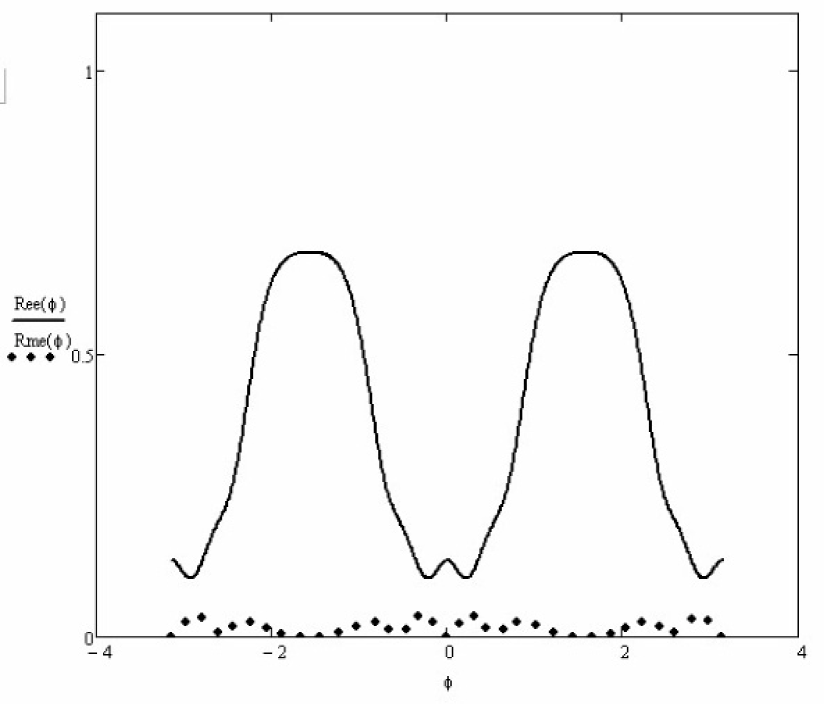
Figure 4: Dependence of reflectivities $|R_{ee}|^{2}$ and $|R_{me}|^{2}$ of an anisotropic plate with $\epsilon_{0}=1.6$, $\eta=0.8$ and dimensionless thickness $L\omega/c=10$ on angle $\phi$ of the plate rotation around its normal, when the anisotropy vector $a$ is parallel to interfaces and at $\phi=0$ is directed along $\mbox{\boldmath$k$}_{\|}$. The incidence angle $\theta$ is given by $\sin\theta=0.9$.

It is very easy to put down a self consistent equation for determination of $|\overrightarrow{x}\rangle$:

$$|\overrightarrow{x}\rangle=\overrightarrow{\mbox{\boldmath$\hat{E}$}}(L)\overrightarrow{\mbox{\boldmath$\hat{\cal T}$}}|\xi_{0}\rangle+\overrightarrow{\mbox{\boldmath$\hat{E}$}}(L)\overleftarrow{\mbox{\boldmath$\hat{\cal R}$}}^{\prime}\overleftarrow{\mbox{\boldmath$\hat{E}$}}(L)\overrightarrow{\mbox{\boldmath$\hat{\cal R}$}}^{\prime}|\overrightarrow{x}\rangle.$$ (78)

The first term at the right hand side describes the incident state transmitted through the first interface and propagated up to the second one. The second term describes contribution to the state $|\overrightarrow{x}\rangle$ of the $|\overrightarrow{x}\rangle$ itself. After reflection from the second interface this state propagates to the left up to the first interface, and after reflection from it propagates back to the point $z=L$. Two terms at the right hand side of (76) add together, which results to some new state. But we denoted it $|\overrightarrow{x}\rangle$, and it explains derivation of the equation (76).

From (76) we can directly find

$$|\overrightarrow{x}\rangle=\Big{[}\mbox{\boldmath$\hat{I}$}-\overrightarrow{\mbox{\boldmath$\hat{E}$}}(L)\overleftarrow{\mbox{\boldmath$\hat{\cal R}$}}^{\prime}\overleftarrow{\mbox{\boldmath$\hat{E}$}}(L)\overrightarrow{\mbox{\boldmath$\hat{\cal R}$}}^{\prime}\Big{]}^{-1}\overrightarrow{\mbox{\boldmath$\hat{E}$}}(L)\overrightarrow{\mbox{\boldmath$\hat{\cal T}$}}|\xi_{0}\rangle,$$ (79)

and substitution into (75) and (76) gives

$$\overrightarrow{\mbox{\boldmath$\hat{T}$}}(L)\equiv\left(\begin{array}[]{cc}T_{ee}&T_{em}\\ T_{me}&T_{mm}\\ \end{array}\right)=\overrightarrow{\mbox{\boldmath$\hat{\cal T}$}}^{\prime}\Big{[}\mbox{\boldmath$\hat{I}$}-\overrightarrow{\mbox{\boldmath$\hat{E}$}}(L)\overleftarrow{\mbox{\boldmath$\hat{\cal R}$}}^{\prime}\overleftarrow{\mbox{\boldmath$\hat{E}$}}(L)\overrightarrow{\mbox{\boldmath$\hat{\cal R}$}}^{\prime}\Big{]}^{-1}\overrightarrow{\mbox{\boldmath$\hat{E}$}}(L)\overrightarrow{\mbox{\boldmath$\hat{\cal T}$}},$$ (80)

$$\overrightarrow{\mbox{\boldmath$\hat{R}$}}(L)\equiv\left(\begin{array}[]{cc}R_{ee}&R_{em}\\ R_{me}&R_{mm}\\ \end{array}\right)=\overrightarrow{\mbox{\boldmath$\hat{\cal R}$}}+\overleftarrow{\mbox{\boldmath$\hat{\cal T}$}}^{\prime}\overleftarrow{\mbox{\boldmath$\hat{E}$}}(L)\overrightarrow{\mbox{\boldmath$\hat{\cal R}$}}^{\prime}\Big{[}\mbox{\boldmath$\hat{I}$}-\overrightarrow{\mbox{\boldmath$\hat{E}$}}(L)\overleftarrow{\mbox{\boldmath$\hat{\cal R}$}}^{\prime}\overleftarrow{\mbox{\boldmath$\hat{E}$}}(L)\overrightarrow{\mbox{\boldmath$\hat{\cal R}$}}^{\prime}\Big{]}^{-1}\overrightarrow{\mbox{\boldmath$\hat{E}$}}(L)\overrightarrow{\mbox{\boldmath$\hat{\cal T}$}}.$$ (81)

With these formulas we can easily calculate all the reflectivities and transmissivities for arbitrary parameters, arbitrary incidence angles, arbitrary incident polarizations and arbitrary direction of the anisotropy vector $a$. In fig.4 we present, for example, reflectivities of TE-mode wave from a plate of thickness $L$ such, that $L\omega/c=10$. The anisotropy vector is parallel to interfaces. Therefore, its orientation with respect to wave vector $\mbox{\boldmath$k$}_{0}$ of the incident wave varies with rotation of the plate by an angle $\phi$ around its normal. The transmissivities of the same plate in dependence on the angle $\phi$ are presented in fig.5.

It is important to note that after transmission through anisotropic plate the transmitted ray has the same angle with the plate normal as the incident one, and it is interesting to investigate how the image of a real object splits, when observed through a birefringent ideal plain plate.

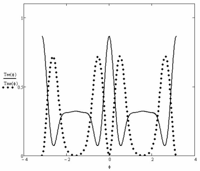
Figure 5: Dependence of transmissivities $|T_{ee}|^{2}$ and $|T_{me}|^{2}$ of an anisotropic plate on angle $\phi$ of the plate rotation around its normal, with all the parameters the same as shown in caption of fig.4.

5 Conclusion

We have shown how to find polarizations of plain waves propagating in a single axis anisotropic media, how to calculate reflection and refraction at an interface between anisotropic and isotropic media, and how to calculate reflection and transmission of plain parallel transparent anisotropic layers. We considered media without absorption, but inclusion of absorption does not provide any problem.

We have shown that reflection from interfaces in anisotropic media is accompanied beam splitting, that reflection of the mixed mode is nonspecular and can be characterized by two critical angles. The first critical angle $\varphi_{c1}$ corresponds to total reflection with nonspecular double beam splitting. The second critical angle corresponds to total nonspecular reflection of mixed mode without beam splitting and creation of surface electromagnetic wave. The effect can be observed with the help of birefringent cone, when the incident beam is transmitted through the side surface and after reflection from the base plane goes out of the cone.

We considered only one anisotropy vector, and it will be a good exercise to consider whether addition of a second anisotropy axis will not bring some new effects.

Appendix A Substitution of mode polarizations in boundary conditions for incident wave of mode 2

A.1 TE-mode

Substitution of (15) for $\mbox{\boldmath$\cal E$}_{2}$, $[\mbox{\boldmath$a$}\times\mbox{\boldmath$\kappa$}]$ for $\mbox{\boldmath$\cal E$}_{1}$ and (25) for $\mbox{\boldmath$\cal H$}_{1,2}$ into (39) and (40) gives

$$(\mbox{\boldmath$t$}\cdot\mbox{\boldmath$a$})+(\mbox{\boldmath$t$}\cdot[\mbox{\boldmath$a$}\times\overleftarrow{\mbox{\boldmath$\kappa$}}_{1}])\overrightarrow{\rho}_{12}+(\mbox{\boldmath$t$}\cdot\mbox{\boldmath$a$})\overrightarrow{\rho}_{22}=\overrightarrow{\tau}_{e2},$$

$$k_{2r\bot}(\mbox{\boldmath$t$}\cdot\mbox{\boldmath$a$})-k_{1\bot}(\mbox{\boldmath$t$}\cdot[\mbox{\boldmath$a$}\times\overleftarrow{\mbox{\boldmath$\kappa$}}_{1}])\overrightarrow{\rho}_{12}-k_{2l\bot}(\mbox{\boldmath$t$}\cdot\mbox{\boldmath$a$})\overrightarrow{\rho}_{22}=k_{0\bot}\overrightarrow{\tau}_{e2},$$

where $\overleftarrow{\mbox{\boldmath$\kappa$}}_{1}=(\mbox{\boldmath$k$}_{\|},-k_{1\bot})/k_{1}$, $k_{1}=k_{0}\sqrt{\epsilon_{0}}$, $k_{1\bot}=\sqrt{k_{1}^{2}-k_{\|}^{2}}$, and $k_{2r,l\bot}$ are given in (30), (32). In equation (39a) we took into account that vector $t$ is orthogonal to $\kappa$, and in (40a) we used representation: $\mbox{\boldmath$\kappa$}=\kappa_{\|}\mbox{\boldmath$l$}+\kappa_{\bot}\mbox{\boldmath$n$}$, and the relation $[\mbox{\boldmath$l$}\times\mbox{\boldmath$n$}]=-\mbox{\boldmath$t$}$, which for any vector $A$ gives

$$(\mbox{\boldmath$l$}\cdot[\mbox{\boldmath$\kappa$}\times\mbox{\boldmath$A$}])=([\mbox{\boldmath$l$}\times\mbox{\boldmath$\kappa$}]\cdot\mbox{\boldmath$A$})=-\kappa_{\bot}(\mbox{\boldmath$t$}\cdot\mbox{\boldmath$A$}).$$ (82)

After exclusion of $\tau_{e2}$ from these equations we obtain the equation

$$(\mbox{\boldmath$t$}\cdot[\mbox{\boldmath$a$}\times\overleftarrow{\mbox{\boldmath$\kappa$}}_{1}])(k_{1\bot}+k_{0\bot})\overrightarrow{\rho}_{12}+(\mbox{\boldmath$t$}\cdot\mbox{\boldmath$a$})(k_{0\bot}+k_{2l\bot})\overrightarrow{\rho}_{22}=(\mbox{\boldmath$t$}\cdot\mbox{\boldmath$a$})(k_{2r\bot}-k_{0\bot}).$$ (83)

In the case of isotropic medium

we have $k_{2r\bot}=k_{2l\bot}=k_{1\bot}=k_{\bot}$, $\overleftarrow{\mbox{\boldmath$\kappa$}}_{1}=\mbox{\boldmath$\kappa$}_{l}=(\mbox{\boldmath$k$}_{\|},-k_{\bot})/k$, therefore (83) is reduced to

$$\frac{(\mbox{\boldmath$t$}\cdot[\mbox{\boldmath$a$}\times\mbox{\boldmath$\kappa$}_{r}])}{(\mbox{\boldmath$t$}\cdot\mbox{\boldmath$a$})}\overrightarrow{\rho}_{12}+\overrightarrow{\rho}_{22}=\rho_{e0},\qquad\overrightarrow{\tau}_{e2}=(\mbox{\boldmath$t$}\cdot\mbox{\boldmath$a$})\tau_{e0},$$ (84)

where

$$\rho_{e0}=\displaystyle\frac{(k_{\bot}-k_{0\bot})}{(k_{\bot}+k_{0\bot})},\qquad\tau_{e0}=1+\rho_{e0}=\displaystyle\frac{2k_{\bot}}{(k_{\bot}+k_{0\bot})}$$ (85)

are the standard reflection and transmission amplitudes [5] of a pure TE-mode at an interface between isotropic media.

If $\mbox{\boldmath$a$}=\mbox{\boldmath$t$}$ we have the typical incident TE-mode, and $\rho_{12}$ is excluded because $(\mbox{\boldmath$t$}\cdot[\mbox{\boldmath$\kappa$}_{r}\times\mbox{\boldmath$a$}])=0$.

If $(\mbox{\boldmath$a$}\cdot\mbox{\boldmath$t$})=0$ we have the typical incident TM-mode, and from (39a), (40a) it follows that $\rho_{12}=0$

A.2 TM-mode

The similar substitutions of $\mbox{\boldmath$\cal H$}_{1,2}$ into (42) for TM-mode gives

$$\frac{k_{2r}}{k_{0}}(\mbox{\boldmath$t$}\cdot[\overrightarrow{\mbox{\boldmath$\kappa$}}_{2}\times\mbox{\boldmath$a$}])+\displaystyle\frac{k_{1}}{k_{0}}(\mbox{\boldmath$t$}\cdot\mbox{\boldmath$a$})\overrightarrow{\rho}_{12}+\displaystyle\frac{k_{2l}}{k_{0}}(\mbox{\boldmath$t$}\cdot[\overleftarrow{\mbox{\boldmath$\kappa$}}_{2}\times\mbox{\boldmath$a$}])\overrightarrow{\rho}_{22}=\overrightarrow{\tau}_{m}.$$

For substitution of $\cal E$ into (43) we represent (15) in the form

$$\mbox{\boldmath$e$}_{2}=[\mbox{\boldmath$\kappa$}\times[\mbox{\boldmath$a$}\times\mbox{\boldmath$\kappa$}]]\displaystyle\frac{\epsilon_{1}(\theta)}{\epsilon_{0}}-\mbox{\boldmath$a$}\displaystyle\frac{\Delta\epsilon(\theta)}{\epsilon_{0}},$$ (86)

where $\Delta\epsilon(\theta)=\epsilon_{1}(\theta)-\epsilon_{0}$, and with account of (82) we obtain

$$\kappa_{2r\bot}(\mbox{\boldmath$t$}\cdot[\overrightarrow{\mbox{\boldmath$\kappa$}}_{2}\times\mbox{\boldmath$a$}])\displaystyle\frac{\epsilon_{1}(\theta_{2r})}{\epsilon_{0}}-\displaystyle\frac{\Delta\epsilon(\theta_{2r})}{\epsilon_{0}}(\mbox{\boldmath$l$}\cdot\mbox{\boldmath$a$})-\kappa_{1\bot}(\mbox{\boldmath$t$}\cdot\mbox{\boldmath$a$})\overrightarrow{\rho}_{12}-$$

$$-\left(\kappa_{2l\bot}(\mbox{\boldmath$t$}\cdot[\overleftarrow{\mbox{\boldmath$\kappa$}}_{2}\times\mbox{\boldmath$a$}])\displaystyle\frac{\epsilon_{1}(\theta_{2l})}{\epsilon_{0}}+\displaystyle\frac{\Delta\epsilon(\theta_{2l})}{\epsilon_{0}}(\mbox{\boldmath$l$}\cdot\mbox{\boldmath$a$})\right)\overrightarrow{\rho}_{22}=\kappa_{0\bot}\overrightarrow{\tau}_{m}.$$

Exclusion of $\overrightarrow{\tau}_{m}$ with the help of (42b) gives

$$(\epsilon_{0}k_{0\bot}k_{2r}+k_{1\bot}k_{1})(\mbox{\boldmath$t$}\cdot\mbox{\boldmath$a$})\overrightarrow{\rho}_{12}+\Big{(}(\epsilon_{0}k_{0\bot}k_{2r}+k_{2l\bot}k_{2l})(\mbox{\boldmath$t$}\cdot[\overleftarrow{\mbox{\boldmath$\kappa$}}_{2}\times\mbox{\boldmath$a$}])+k_{0}^{2}\Delta\epsilon(\theta_{2l})(\mbox{\boldmath$l$}\cdot\mbox{\boldmath$a$})\Big{)}\overrightarrow{\rho}_{22}=$$

$$=k_{2r}(k_{2r\bot}-\epsilon_{0}k_{0\bot})(\mbox{\boldmath$t$}\cdot[\overrightarrow{\mbox{\boldmath$\kappa$}}_{2}\times\mbox{\boldmath$a$}])-k_{0}^{2}\Delta\epsilon(\theta_{2r})(\mbox{\boldmath$l$}\cdot\mbox{\boldmath$a$}).$$ (87)

Together with (83) we have two equations for determination of $\rho_{22}$ and $\rho_{12}$.

In the case of isotropic medium

we have $k_{2r\bot}=k_{2l\bot}=k_{1\bot}=k_{\bot}$, $k_{2r}=k_{2l}=k_{1l}=k$, $\Delta\epsilon=0$, $\epsilon_{1}=\epsilon_{0}$, $\overrightarrow{\mbox{\boldmath$\kappa$}}_{2}=\overrightarrow{\mbox{\boldmath$\kappa$}}=(\mbox{\boldmath$k$}_{\|},k_{\bot})/k$, $\overleftarrow{\mbox{\boldmath$\kappa$}}_{2}=\overleftarrow{\mbox{\boldmath$\kappa$}}_{1}=\overleftarrow{\mbox{\boldmath$\kappa$}}=(\mbox{\boldmath$k$}_{\|},-k_{\bot})/k$. Therefore (87) is reduced to

$$(\mbox{\boldmath$t$}\cdot\mbox{\boldmath$a$})\overrightarrow{\rho}_{12}+(\mbox{\boldmath$t$}\cdot[\overleftarrow{\mbox{\boldmath$\kappa$}}\times\mbox{\boldmath$a$}])\overrightarrow{\rho}_{22}=(\mbox{\boldmath$t$}\cdot[\overrightarrow{\mbox{\boldmath$\kappa$}}\times\mbox{\boldmath$a$}])\displaystyle\frac{(k_{\bot}-\epsilon_{0}k_{0\bot})}{(k_{\bot}+\epsilon_{0}k_{0\bot})}\equiv(\mbox{\boldmath$t$}\cdot[\overrightarrow{\mbox{\boldmath$\kappa$}}\times\mbox{\boldmath$a$}])\rho_{m0},$$ (88)

and solution of (88) with (84) gives

$$\overrightarrow{\rho}_{12}=\displaystyle\frac{(\mbox{\boldmath$t$}\cdot\mbox{\boldmath$a$})\left((\mbox{\boldmath$t$}\cdot[\overrightarrow{\mbox{\boldmath$\kappa$}}\times\mbox{\boldmath$a$}])\rho_{m0}-(\mbox{\boldmath$t$}\cdot[\overleftarrow{\mbox{\boldmath$\kappa$}}\times\mbox{\boldmath$a$}])\rho_{e0}\right)}{(\mbox{\boldmath$t$}\cdot[\overleftarrow{\mbox{\boldmath$\kappa$}}\times\mbox{\boldmath$a$}])^{2}+(\mbox{\boldmath$t$}\cdot\mbox{\boldmath$a$})^{2}},$$ (89)

$$\overrightarrow{\rho}_{22}=\displaystyle\frac{(\mbox{\boldmath$t$}\cdot[\overleftarrow{\mbox{\boldmath$\kappa$}}\times\mbox{\boldmath$a$}])(\mbox{\boldmath$t$}\cdot[\overrightarrow{\mbox{\boldmath$\kappa$}}\times\mbox{\boldmath$a$}])\rho_{m0}+(\mbox{\boldmath$t$}\cdot\mbox{\boldmath$a$})^{2}\rho_{e0}}{(\mbox{\boldmath$t$}\cdot[\overleftarrow{\mbox{\boldmath$\kappa$}}\times\mbox{\boldmath$a$}])^{2}+(\mbox{\boldmath$t$}\cdot\mbox{\boldmath$a$})^{2}}.$$ (90)

For $\tau_{m}$ it follows from (42a) that

$$\overrightarrow{\tau}_{m}=(\mbox{\boldmath$t$}\cdot[\overrightarrow{\mbox{\boldmath$\kappa$}}\times\mbox{\boldmath$a$}])(1+\rho_{m0})=(\mbox{\boldmath$t$}\cdot[\overrightarrow{\mbox{\boldmath$\kappa$}}\times\mbox{\boldmath$a$}])\displaystyle\frac{2k_{\bot}}{k_{\bot}+\epsilon_{0}k_{0\bot}}\equiv(\mbox{\boldmath$t$}\cdot[\overrightarrow{\mbox{\boldmath$\kappa$}}\times\mbox{\boldmath$a$}])\tau_{m0},$$

where $\rho_{m0}$ and $\tau_{m0}$ are the standard reflection and transmission amplitudes [5] of a pure TM-mode at an interface between isotropic media.

Thus, for an internal reflection from an interface of isotropic dielectric with vacuum we obtained reflection and refraction amplitudes for an incident field with an arbitrary polarization $\mbox{\boldmath$e$}=[\mbox{\boldmath$\kappa$}\times[\mbox{\boldmath$a$}\times\mbox{\boldmath$\kappa$}]]$, which is determined by some unit vector $a$. If $\mbox{\boldmath$a$}=\mbox{\boldmath$t$}$, then $\overrightarrow{\rho}_{12}=0$ and $\overrightarrow{\rho}_{22}=\rho_{e0}$. If $(\mbox{\boldmath$a$}\cdot\mbox{\boldmath$t$})=0$, then again $\overrightarrow{\rho}_{12}=0$, but $\overrightarrow{\rho}_{22}=\rho_{m0}(\mbox{\boldmath$t$}\cdot[\overrightarrow{\mbox{\boldmath$\kappa$}}\times\mbox{\boldmath$a$}])/(\mbox{\boldmath$t$}\cdot[\overleftarrow{\mbox{\boldmath$\kappa$}}\times\mbox{\boldmath$a$}])$. If $\mbox{\boldmath$a$}=\overleftarrow{\mbox{\boldmath$\kappa$}}$, then $\overrightarrow{\rho}_{22}$ is divergent, however the reflected field $\overleftarrow{\mbox{\boldmath$\cal E$}}_{2}\overrightarrow{\rho}_{22}$ has the finite value $\rho_{m0}(\mbox{\boldmath$t$}\cdot[\overrightarrow{\mbox{\boldmath$\kappa$}}\times\mbox{\boldmath$a$}])$.

Appendix B History of submission and rejection

The paper was submitted to Am.J.Phys on September 1 of 2010. It was rejected on September 24 because of negative reports of two referees. The first referee said that he is lazy to read the manuscript with pencil, but he saw that sections 2 and 4 are absolutely not needed, because everything about reflections is much better said in textbooks by Jackson and Griffith. The second referee rejected because we, he said, erroneously told that the recent paper was publish long ago at 1977. He said that since then there were many papers on optical reflection and transmission.

If we could reply to referee we would mention that in textbooks by Jackson and Griffith there are no word on anisotropic media. The referee overlooked the main point of our paper. As for claim of the second referee, we would like to say, that he can try to seek on AJP home page a paper with key words “electromagnetic waves in anisotropic media.” Then he will find the first article published in 1977. So the second referee also overlooked the main point of our article.

References

• [*] e-mail: v.ignatovi@gmail.com
• [1] F.I.Fedorov, Optics of anisotropic media, Minsk, BSSR Ac.Sc., 1958. Eq. (20.4)
• [2] Petr KuzΜ†hel, β€œLecture 8: Light propagation in anisotropic media”,
http://www.fzu.cz/Β kuzelp/Optics/Lectures.htm;
http://www.fzu.cz/Β kuzelp/Optics/Lecture8.pdf
• [3] Petr KuzΜ†hel, Electromagnetisme des milieux continus. β€œOptique”, Universite Paris-Nord, 2000/2001.
• [4] R.W.Ditchburn. Light, Dover Publications Inc.N.Y. 1991.
• [5] L. D. Landau, E. M. Lifshitz and L. P. Pitaevskii, Electrodynamics of Continuous Media. Second Edition: Volume 8 (Course of Theoretical Physics) Elsevier Butterworth-Heinemann, 2004. Ch.XI.
• [6] K.S.Kunz. β€œTreatment of optical propagation in crystals using projection dyadics.” Am.J.Phys. 45 267 (1977).
• [7] Vladimir K. Ignatovich, Loan T. N. Phan, Those wonderful elastic waves. Am. J. Phys. 77 1162 (2009)
• [8] Vladimir K. Ignatovich, Masahiko Utsuro, Handbook on Neutron Optics, Wiley-VCN Verlag GmbH, & Co. KGaA, 2009.