Deconvolution of window effect in galaxy power spectrum analysis

Abstract

We develop a new method for deconvolving the smearing effect of the survey window in the analysis of the galaxy multipole power spectra from a redshift survey. This method is based on the deconvolution theorem, and is compatible with the use of the fast Fourier transform. It is possible to measure the multipole power spectra deconvolved from the window effect efficiently. Applying this method to the luminous red galaxy sample of the Sloan Digital Sky Survey data release 7 as well as mock catalogues, we demonstrate how the method works properly. Using this deconvolution technique, the amplitude of the multipole power spectrum is corrected. Besides, the covariance matrices of the deconvolved power spectra get quite close to the diagonal form. This is also advantageous in the study of the BAO signature.

1 Introduction

The power spectrum is one of the most fundamental tools to characterize the large-scale clustering of galaxies (e.g., Dodelson). The role of the power spectrum analysis in cosmology is becoming more and more important [2]. Especially, the power spectrum of galaxies plays a key role for extracting the baryon acoustic oscillations (BAO) [3, 4, 5], which is essential for the dark energy research. The quadruple power spectrum is also useful for measuring the redshift-space distortion, which plays a vital role of testing gravity on the scales of cosmology [6, 7, 8].

The method developed by Feldman, Kaiser and Peacock (hereafter FKP, FKP94) is often adopted to measure the power spectrum [5]. It is known that the power spectrum measured using the FKP method, due to finiteness of the survey volume, is convolved with a window function. This convolution is expressed schematically as,

$$P^{\rm conv}({\bf k})={1\over(2\pi)^{3}}\int d^{3}k^{\prime}P({\bf k}^{\prime})W({\bf k}-{\bf k}^{\prime}),$$ (1)

where ${\bf k}$ is the wavenumber vector, $W({\bf k}-{\bf k}^{\prime})/(2\pi)^{3}$ describes the survey window, and we refer to $P^{\rm conv}({\bf k})$ as the ‘convolved’ power spectrum. In the limit of an infinitely large survey volume, $W({\bf k}-{\bf k}^{\prime})/(2\pi)^{3}$ approaches the three dimensional delta function, hence $P^{\rm conv}({\bf k})$ becomes the same as the true power spectrum $P({\bf k})$.

In a realistic case, however, a survey volume is finite. The window convolution modifies a measured power spectrum compared with the true power spectrum. It has the following two aspects: (i) change of the amplitude of the power spectrum, (ii) mixing of modes with different wavenumbers. These two effects are influential in the power spectrum analysis for extracting the BAO and in testing gravity on the scales of cosmology. When comparing the convolved power spectrum with theoretical predictions, we need to take the window effect into account following Eq. (1), even though it is quite a time consuming process [10].

If we could directly measure a deconvolved power spectrum from a galaxy data, it could be compared with theoretical models without including the window effect [11], thus speeding up the analysis significantly. In the present paper, for the first time, we develop a scheme to measure the deconvolved multipole power spectra. We apply it to the Sloan Digital Sky Survey (SDSS) luminous red galaxy (LRG) sample from the data release (DR) 7 as well as to $1000$ mock catalogues mimicking the LRG sample. This paper is organised as follows: In section 2, we present a new method to deconvolve the window function from the FKP estimator, including a brief review for the FKP estimator for the power spectrum. In section 3, we apply the method to the SDSS LRG DR7 as well as to $1000$ mock catalogues, and demonstrate how it works in the multipole power spectrum analysis, by comparing the convolved power spectrum and the deconvolved power spectrum. Throughout this paper, we use units in which the velocity of light equals 1, and adopt the Hubble parameter $H_{0}=100h$ km/s/Mpc with $h=0.7$.

2 Formulation

Here we provide basic formulas for the deconvolution of the window function. Taking the Fourier transformation of Eq. (1), we have

$$\int d^{3}{k}e^{-i{\bf k}\cdot{\bf s}}P^{\rm conv}({\bf k})={1\over(2\pi)^{3}}\left[\int d^{3}k^{\prime}e^{-i{\bf k}^{\prime}\cdot{\bf s}}P({\bf k}^{\prime})\right]\left[\int d^{3}ke^{-i{\bf k}\cdot{\bf s}}W({\bf k})\right].$$ (2)

This can be done exactly as long as the k-space is infinitely large. Then, we have

$$\int d^{3}k^{\prime}e^{-i{\bf k}^{\prime}\cdot{\bf s}}P({\bf k}^{\prime})=(2\pi)^{3}{\displaystyle{\int d^{3}{k^{\prime}}e^{-i{\bf k}^{\prime}\cdot{\bf s}}P^{\rm conv}({\bf k}^{\prime})}\over\displaystyle{\int d^{3}k^{\prime\prime}e^{-i{\bf k}^{\prime\prime}\cdot{\bf s}}W({\bf k}^{\prime\prime})}},$$ (3)

whose inverse transformation yields

$$P({\bf k})=\int d^{3}se^{i{\bf k}\cdot{\bf s}}{\displaystyle{\int d^{3}{k^{\prime}}e^{-i{\bf k}^{\prime}\cdot{\bf s}}P^{\rm conv}({\bf k}^{\prime})}\over\displaystyle{\int d^{3}k^{\prime\prime}e^{-i{\bf k}^{\prime\prime}\cdot{\bf s}}W({\bf k}^{\prime\prime})}}.$$ (4)

For a discrete density field, we need to subtract the shot-noise contribution. Following the FKP method, the estimator of the convolved power spectrum is

$$P^{\rm conv}({\bf k})={\bigl{|}\int d^{3}s\psi({\bf s})[n_{\rm g}({\bf s})-\alpha n_{\rm rnd}({\bf s})]e^{i{\bf k}\cdot{\bf s}}\bigr{|}^{2}\over[\int d^{3}s\bar{n}^{2}({\bf s})\psi^{2}({\bf s})]}-(1+\alpha)S_{0},$$ (5)

where $n_{\rm g}({\bf s})$ is the number density field of galaxies whose mean number density is $\bar{n}({\bf s})$, $n_{\rm rnd}({\bf s})$ is the density field of a random sample whose mean number density is $\alpha^{-1}\bar{n}({\bf s})$, $\psi({\bf s})$ is the weight factor, ${\bf s}$ denotes the three dimensional coordinate of the redshift-space, and we defined

$$S_{0}={\int d^{3}s\bar{n}({\bf s})\psi^{2}({\bf s})\over\int d^{3}s\bar{n}^{2}({\bf s})\psi^{2}({\bf s})},$$ (6)

which describes the shot-noise contribution. The random catalogue is a set of random points without any correlation, which can be constructed through a random process by mimicking the selection function of the galaxy catalogue. Note that $\alpha$ is the parameter of the random catalogue, for which we adopt the value of $0.01$, in the present paper. Similarly, we may adopt the estimator for the window function

$$W({\bf k})={\big{|}\int d^{3}s\alpha n_{\rm rnd}({\bf s})\psi({\bf s})e^{i{\bf s}\cdot{\bf k}}\big{|}^{2}\over\int d^{3}s\bar{n}^{2}({\bf s})\psi^{2}({\bf s})}-\alpha S_{0}.$$ (7)

Note that the denominator $\int d^{3}s\bar{n}^{2}({\bf s})\psi^{2}({\bf s})$ cancels out when we substitute Eqs. (5), (6) and (7) into Eq. (4). Practically, the computation of $W({\bf k})$ must be done carefully, because it might become zero when we choose a box size for the fast Fourier transform too large. One can avoid this problem by properly choosing the box size in which sample galaxies are distributed.

The monopole power spectrum is computed from Eq. (4),

$$P_{0}(k)={1\over V_{k}}\int_{V_{k}}d^{3}kP({\bf k}),$$ (8)

where $V_{k}$ is the volume of a shell in the Fourier space, whose mean radius is $k$. Within the small-angle approximation (distant observer approximation), the estimator of the higher multipole power spectra might be taken as

$$P_{\ell}(k)={1\over V_{k}}\int_{V_{k}}d^{3}kP({\bf k}){\cal L}_{\ell}({\bf\hat{e}}\cdot{\bf\hat{k}}),$$ (9)

where $\hat{\bf e}$ denotes the unit vector that points to line of sight direction, ${\cal L}_{\ell}(\mu)$ is the Legendre polynomial, and $\hat{\bf k}={\bf k}/|{\bf k}|$ is the unit wavenumber vector. Note that the line of sight direction is approximated by one direction $\hat{\bf e}$ in this approach. We refer to the multipole power spectrum $P_{\ell}(k)$ with Eq. (4) substituted into the right hand side of (9) as the ‘deconvolved’ multipole power spectrum. Note that our definition of the multipole spectrum $P_{\ell}(k)$ is different from the conventional one by the factor $2\ell+1$ [12, 13].

In the ref. YNKBN, the FKP method is generalized to measure higher order multipole power spectra, which is useful in quantifying the redshift-space distortions (cf. CFW,Hamilton). There are differences between the previous paper [14] and the present one in the estimators for the higher multipole spectra. In Table I, the differences of the two approaches are summarized. In the previous paper [14], the line of sight direction was defined for each pair of galaxies, while in the present paper the line of sight direction is approximated by only one direction $\hat{\bf e}$. In this sense, the approximation of the present paper is limited to a set of galaxies within a narrow survey area. A similar approach was adopted in the references OutramI,OutramII. In this approach, because of the limitation of the small-angle approximation, a full sample of large survey area must be divided into subsamples of narrow survey areas. Because of the division of the full sample, the window effect could be very influential, but the advantage of this approach is that one can use the fast Fourier transform.

	Present paper	Reference YNKBN
Line of sight direction	approximated by	computed for each
	one direction $\hat{\bf e}$	pair of galaxies
Division of galaxy sample	necessary	not necessary
Window effect	significant	not significant
Use of the fast Fourier transform	possible	impossible

Table 1: Comparison of the two approaches

3 Application

In this section we apply our method to the SDSS LRG sample of DR7. Our LRG sample is restricted to the redshift range $z=0.16$ - $0.47$. In order to reduce the sidelobes of the survey window we remove some non-contiguous parts of the sample, which leads us to 7150 deg² sky coverage with the total number $N=100157$ LRGs. The data reduction is the same as that described in the references Hutsia,Yamamoto10. In our power spectrum analysis we adopt the spatially flat lambda cold dark matter model distance-redshift relation with $\Omega_{m}=0.28$, and set $\psi=1$.

We divide the full sample into subsamples, in which galaxies are distributed within narrow area. This is necessary to compute the quadrupole power spectrum in our method with the fast Fourier transform. In the present paper, we divide the full sample into $18$ subsamples whose area and numbers of galaxies are almost equal, $397$ square degrees, or into $32$ subsamples whose mean area is $223$ square degrees.

3.1 Shape of the multipole power spectrum

First, we focus on the shapes of the monopole and the quadrupole power spectra. Figure 1 shows the convolved (left panels) and deconvolved (right panels) power spectra from the SDSS LRG sample. The upper left panel plots the convolved monopole spectrum multiplied by the wavenumber, $kP^{\rm conv}_{0}(k)$. Here the following two cases are shown: (i) the full sample divided into 18 subsamples with each piece spanning almost $397$ square degrees, (ii) the full sample without division into subsamples. Due to significantly different effect of the window convolution in these two cases, the amplitude of the two spectra are very different. The upper right panel is the same as the upper left panel, but is the deconvolved power spectrum $kP_{0}(k)$. Note that, in this panel, the amplitudes of the two deconvolved spectra are almost the same. The lower panels plot $kP_{2}(k)$. The left panel is the convolved spectrum, while the right panel is the deconvolved spectrum. For the quadrupole power spectrum, we present the two cases with different divisions: chunks with mean survey area $397$ square degrees, and $223$ square degrees, respectively. One can see the same features as those for $kP_{0}(k)$. The results do not depend on the division of the full sample. The error-bars are obtained by computing the standard deviations of 1000 mock catalogues (A), explained in the next.

Figure 2 is the same as figure 1, but shows the average from 1000 mock catalogues (A), which are obtained by the following three steps, whose details are described in the reference Hutsia. First, we generate the density field using an optimized 2nd order Lagrangian perturbation calculation. Second, we take the Poisson sampling of the generated density field, adjusting the clustering bias and the number density so as to agree with the observed LRG sample. Third, we apply the radial and angular selection function, and extract the final catalogues. We call these mock catalogues (A). Figure 2 clearly shows that the amplitudes of the two deconvolved spectra are almost the same.

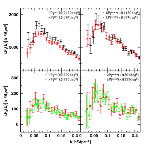
Figure 1: Comparison of the convolved $kP_{\ell}^{\rm conv}(k)$ (left panel) and deconvolved power spectra $kP_{\ell}(k)$ (right panel). The upper panels plot the monopole $\ell=0$, while the lower ones the quadrupole $\ell=2$. For the monopole power spectrum, the two cases are presented: One is the case when the full sample is divided into $18$ subsamples and the other is the case without division of the full sample. For the quadrupole spectrum, the two different cases of the division of the full sample are presented, in which the mean survey areas are $397$ square degrees and $223$ square degrees, respectively. The error-bars are obtained by computing the standard deviations of 1000 mock catalogues (A).

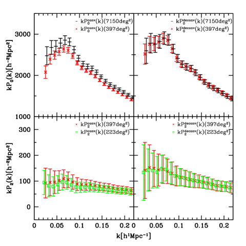
Figure 2: Same as figure 1 but using the average from $1000$ mock catalogues (A). The error-bars are the standard deviations.

Figure 3 demonstrates how the deconvolution recovers the original power spectrum properly. To this end, we buid other catalogues (B) and (C). The cosmological parameters are the same as those of the mock catalogues (A). To buid the catalogues (B), the first step is the same as those for the mock catalogues (A), we generate the density field using an optimized 2nd order Lagrangian perturbation calculation. Then, we take the Poisson sampling of the generated density field, adjusting the clustering bias and the number density. Here, we assumed the homogeneous mean number density with $\bar{n}=8\times 10^{-5}~{}(h^{-1}{\rm Mpc})^{-3}$ in the square region $2560h^{-1}{\rm Mpc}\times 2560h^{-1}{\rm Mpc}\times 1280h^{-1}{\rm Mpc}$. The catalogues (B) are obtained by applying the same selection of the survey region as the SDSS LRG sample. Hence, (B) has the same survey region as (A) but with the constant mean number density.

We also consider the catalogues (C), which are the same as (B) but without the selection of the survey region. Hence, each catalogue of (C) has the square region $2560h^{-1}{\rm Mpc}\times 2560h^{-1}{\rm Mpc}\times 1280h^{-1}{\rm Mpc}$. To obtain the redshift-space catalogues, however, for the catalogues (C), we assume an observer at an infinite distance away, in order to guarantee the validity of the distant observer approximation. Thus the catalogues (C) are ideal samples that assume the large volume and the validity of the distant observer approximation, which could be expected to give us the original power spectrum.

Figure 3 plots the convolved spectra (left panels) and the deconvolved spectra (right panels) from the catalogues (B). The upper panels are the monopole, while the lower panels the quadrupole spectra. In each panel, the convolved spectrum (dotted curve) and the deconvolved spectrum (solid curve) from the ideal catalogues (C) are shown for comparison. These two curves are almost same, hence the convolved spectrum and the deconvolved spectrum are almost same, because the catalogues (C) are ideal samples with the large volume. In the right panels of Fig. 3, the good agreement of all the spectra indicates that our deconvolution recovers the original power spectrum properly. However, one can see small deviation in the quadrupole spectrum between the result from the catalogues (B) and (C), in the lower right panel. As the deviation is larger at small $k$, one possible reason of this small deviation is the limitation of the distant observer approximation for the catalogue (B).

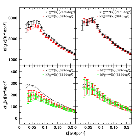
Figure 3: Same as figure 1 but using the average from the $1000$ catalogues (B). The solid curve and the dotted curve are the deconvolved spectrum and the convolved spectrum from the catalogues (C).

3.2 Covariance matrix

In the following we discuss the effect of the deconvolution on the covariance matrix, which is defined by

$${C}_{\ell\ell^{\prime}}(k_{i},k_{j})=\left<\Delta P_{\ell}(k_{i})\Delta P_{\ell^{\prime}}(k_{j})\right>.$$ (10)

We obtain the covariance matrix $C_{\ell\ell^{\prime}}$ using $1000$ mock catalogues. The correlation matrix, which describes the correlation of the errors between different wavenumbers, is defined

$$r_{\ell\ell^{\prime}}(k_{i},k_{j})={C_{\ell\ell^{\prime}}(k_{i},k_{j})\over\sqrt{C_{\ell\ell}(k_{i},k_{i})C_{\ell^{\prime}\ell^{\prime}}(k_{j},k_{j})}}.$$ (11)

Figure 5 shows the correlation matrices of the convolved power spectra for $\ell=\ell^{\prime}=0$ (left panel), $\ell=\ell^{\prime}=2$ (center panel) and $\ell=0,\ell^{\prime}=2$ (right panel), respectively, from the mock catalogue (A). Here, the full sample is divided into 18 subsamples, whose mean survey area is $397$ square degrees. On the other hand, Figure 5 shows the correlation matrices of the deconvolved power spectra for $\ell=\ell^{\prime}=0$ (left panel), $\ell=\ell^{\prime}=2$ (center panel) and $\ell=0,\ell^{\prime}=2$ (right panel) respectively, from the mock catalogue (A). The narrower subsample has a window function with a broader width, which makes the power spectrum at different wavenumbers more strongly correlated. One can see that the errors of the power spectra at different wavenumbers are correlated in figure 5, while practically de-correlated in figure 5. The off-diagonal components of figure 5 are much smaller than those of figure 5.

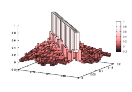
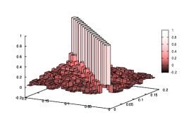
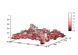
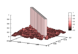
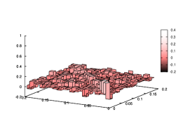
Figure 4: The correlation matrices defined by Eq. (11), obtained from $1000$ mock catalogs: $r_{00}(k,k^{\prime})$ (left panel), $r_{22}(k,k^{\prime})$ (center panel) and $r_{02}(k,k^{\prime})$ (right panel), respectively. Here we used the convolved power spectra of the subsamples with the mean survey area $397$ deg².

Figure 5: Same as figure 5 but with the deconvolved power spectra.

3.3 Baryon acoustic oscillation

In this subsection, we discuss the effect of deconvolution on the BAO signature. In general, the BAO signature in a convolved power spectrum is smoothed compared with the original power spectrum. Then, it is expected that the BAO signature of the deconvolved power spectrum has a larger amplitude compared to that of the convolved power spectrum.

Figure 6 shows the BAO signature of the convolved and deconvolved power spectra from the LRG sample (left panels) and from $1000$ catalogues (B) (right panels), respectively. In each panel, the solid curve and the dotted curve is the BAO signature from the deconvolved spectrum and the convolved spectrum, respectively, obtained with $1000$ ideal catalogues (C). The dashed curve is the theoretical curve in the linear theory.

The results labelled by (1) and (2) are obtained using the full sample without division into subsamples. (1) is from the deconvolved power spectrum $P_{0}(k)$, while (2) is the convolved spectrum $P^{\rm conv}_{0}(k)$. The BAO signature is obtained using the no-wiggle power spectrum multiplied by a function of the form $a+bk+ck^{2}+d/k^{2}$, where $a$, $b$, $c$, and $d$ are fitting parameters (see ref.Nakamura for details). The errors in the left panels are large, but the following features can be seen in the right panels (the results from $1000$ mock catalogues (B)). The difference between (1) and (2) is small, which means that the window effect is not very influential in this case because the survey volume of the full SDSS LRG sample is large. The difference between (1) and the solid curve and the dotted curve is also small. This means that the BAO signature of the deconvolved spectrum (1) well agrees with the original BAO signature.

The results labelled by (3) and (4) are obtained using $18$ subsamples divided from the full sample. (3) is from the deconvolved power spectrum, while (4) from the convolved one, respectively. The difference between (3) and (4) is not negligible at the peaks and the troughs due to the window effect, while the difference between (3) and the solid curve and the dotted curve is small. This means that the deconvolution is successful and recovers the BAO signature, although the window effect is substantial, and degrades the BAO signature when the survey volume is small. Practically, we need not divide a full sample into subsamples to obtain the BAO signature from the monopole spectrum. Then, the window effect on the BAO analysis seems to be small compared with errors. However, in a future precise measurement of the BAO signature, the prescription for the window effect might become important.

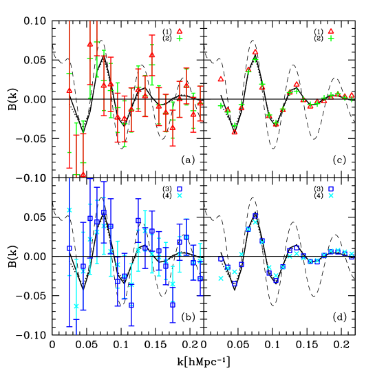
Figure 6: Baryon acoustic oscillation signature of the convolved and deconvolved power spectra from the LRG sample (left panels) and $1000$ mock catalogues (B) (right panels), respectively. In each panel, the solid curve and the dotted curve is from the deconvolved spectrum and the convolved spectrum of the ideal catalogues (C). (1) and (2) are obtained using the full sample without division into subsamples. (1) denoted by $\triangle$ is from the deconvolved power spectrum $P_{0}(k)$, while (2) denoted by $+$ is from the convolved spectrum $P^{\rm conv}_{0}(k)$. The results labelled by (3) and (4) are obtained using $18$ subsamples divided from the full sample. (3) denoted by $\square$ is from the deconvolved power spectrum, while (4) denoted by $\times$ is from the convolved spectrum, respectively. The dashed curve is the theoretical curve in the linear theory.

4 Summary and conclusions

Large galaxy surveys are promising tools for the future dark energy research. In a redshift survey, the power spectrum analysis is very fundamental for extracting the BAO signature. Similarly, tests of the general relativity on the scales of cosmology are becoming important related to this topic in cosmology. This is because a modification of the gravity theory is an alternative way to explain the cosmic acceleration, instead of introducing the dark energy component. The key to distinguish between the dark energy and the modified gravity is the evolution of the cosmological perturbations. The redshift-space distortion caused by the peculiar motions of the galaxies, provides us a useful chance to test gravity on the scale of cosmology [8, 17]. Here the multipole power spectrum plays a key role.

In this paper, we developed a new method to measure the deconvolved power spectra. By applying it to the SDSS DR7 LRG sample as well as to the mock catalogues, we demonstrated that the scheme works well. By the deconvolution, we can get the power spectra whose amplitudes are properly recovered. This will be essential in measuring the redshift-space distortions. The covariance matrices of the deconvolved power spectra are practically diagonal. This is also useful in the study of the BAO signature. Our method matches with the fast Fourier transform, which saves computation time significantly.

As mentioned at the end of the subsection 3.1, the limitation of the distant observer approximation might cause a small deviation of the quadrupole power spectrum when compared with theoretical prediction derived on the basis of the distant observer approximation. For a precise treatment, the framework of the spherical redshift-space distortion is necessary [19, 20]. However, this problem might be softer for a galaxy sample at higher redshift, because a volume within a small angular area can be large.

Acknowledgement This work was supported by Japan Society for Promotion of Science (JSPS) Grants-in-Aid for Scientific Research (Nos. 21540270, 21244033). This work is also supported by JSPS Core-to-Core Program “International Research Network for Dark Energy”. We thank G. Nakamura and A. Taruya for useful discussions.

References

- [1] S. Dodelson, Modern Cosmology (Academic Press, 2003)
- [2] M. Tegmark, et al., Phys. Rev. D 74 (2006), 123507
- [3] G. Hütsi, Astron. Astrophys. 449 (2006), 891
- [4] G. Hütsi, Astron. Astrophys. 459 (2006), 375
- [5] W. Percival, et al., Astrophys. J. 657 (2007), 645; W. Percival, et al., Mon. Not. Roy. Astron. Soc. 381 (2007), 1053; W. Percival, et al., Mon. Not. Roy. Astron. Soc. 401 (2010), 2148
- [6] E. V. Linder, Astropart. Phys. 29 (2008), 336
- [7] L. Guzzo et al., Nature 451 (2008), 541
- [8] K. Yamamoto, T. Sato and G. Hütsi Prog. Theor. Phys. 120 (2008), 609
- [9] H. A. Feldman, N. Kaiser and J. A. Peacock, Astrophys. J. 426 (1994), 23
- [10] T. Sato, G. Hütsi, G. Nakamura and K. Yamamoto, (unpublished)
- [11] K. Fisher, M. Davis, M. A. Strauss, A. Yahil and J. P. Muchra, Astrophys. J. 402 (1993), 42
- [12] S. Cole, K. Fisher and D. H. Weinberg, Mon. Not. Roy. Astron. Soc. 267 (1994), 785
- [13] A. J. S. Hamilton, in The Evolving Universe (Dordrecht: Kluwer Academic Publishers, 1998), 185
- [14] K. Yamamoto, M. Nakamichi, A. Kamino, B. A. Bassett and H. Nishioka, Publ. Astron. Soc. Japan 58 (2006), 93
- [15] P. J. Outram, et al., Mon. Not. Roy. Astron. Soc. 328 (2001), 174
- [16] P. J. Outram, et al., Mon. Not. Roy. Astron. Soc. 348 (2004), 745
- [17] K. Yamamoto, G. Nakamura, G. Hütsi, T. Narikawa and T. Sato, Phys. Rev. D 81 (2010), 103517
- [18] G. Nakamura, G. Hütsi, T. Sato and K. Yamamoto, Phys. Rev. D 80 (2009), 123524
- [19] A. J. S. Hamilton and M. Culhane, Mon. Not. Roy. Astron. Soc. 278 (1996), 73
- [20] A. Raccanelli, L. Samushia and W. J. Percival, Mon. Not. Roy. Astron. Soc., in press, arXiv:1006.1652