Statistical mechanics of collisionless orbits. II. Structure of halos

Abstract

In this paper, we present the density, $\rho$, velocity dispersion, $\sigma$, and $\rho/\sigma^{3}$ profiles of isotropic systems which have the energy distribution, $N(\varepsilon)\propto[\exp(\phi_{0}-\varepsilon)-1]$, derived in Paper I. This distribution, dubbed DARKexp, is the most probable final state of a collisionless self-gravitating system, which is relaxed in terms of particle energies, but not necessarily in terms of angular momentum. We compare the DARKexp predictions with the results obtained using the extended secondary infall model (ESIM). The ESIM numerical scheme is optimally suited for the purpose because (1) it relaxes only through energy redistribution, leaving shell/particle angular momenta unaltered, and (2) being a shell code with radially increasing shell thickness it has very good mass resolution in the inner halo, where the various theoretical treatments give different predictions. The ESIM halo properties, and especially their energy distributions, are very well fit by DARKexp, implying that the techniques of statistical mechanics can be used to explain the structure of relaxed self-gravitating systems.

1 Introduction

Non-relativistic gravitational problems have been the subject of numerous studies, going back to Newton. Despite the simplicity of the force law, these problems vary greatly in the degree of difficulty. The two-body problem is easy and the three-body problem has solutions if certain simplifying assumptions are made, while higher $N$ problems have no useful analytical solutions. When $N$ is large, one can distinguish two types of problems. In the many-body problem, the potential is grainy on scales comparable to the particle separation, while in the infinitely many body problem the potential is smooth on particle scales but can exhibit larger scale fluctuations. It is this last problem which is relevant to the collisionless stellar and dark matter systems, and in this series of papers we concentrate on this problem.

To solve it, one can either numerically integrate individual particle orbits and measure the properties of the evolved system or appeal to the large-$N$ aspect of the problem and attempt to deduce the global properties of the systems, for example, the distribution function. The first approach is taken by the N-body simulations, which in the last couple of decades have produced consistent and robust results for the structure of collisionless dark matter halos (see Navarro et al. (2004) and Stadel et al. (2009), and references therein). These results are widely used in the literature whenever the properties of dark matter halos are called for. Examples of the second, mostly analytical approach can be found in Lynden-Bell (1967); Binney (1982); Stiavelli & Bertin (1987); Merritt et al. (1989); Hjorth & Madsen (1991) and Spergel & Hernquist (1992). While these do reproduce the general features of collisionless systems, they often use the knowledge of the final system (for example, the de Vaucouleurs profile of ellipticals) to motivate the choice of the distribution function. Since simulations make no such assumptions, and have convincingly demonstrated that the end result of collisionless relaxation is the universal profile, is an analytical derivation even needed? We argue that it is.

In this series of papers, we develop an analytical approach, starting from first principles which predicts the properties of relaxed self-gravitating collisionless systems, and test it against numerically evolved systems. In Paper I (Hjorth & Williams, 2010) we showed that if one uses the techniques of statistical mechanics, and works in energy, or orbit space, instead of the usual phase-space, then the standard entropy maximization procedure yields the most probable state described by an exponential differential energy distribution, $N(\varepsilon)\propto\exp(\phi_{0}-\varepsilon)$, where $\varepsilon$ and $\phi_{0}$ are the dimensionless (positive) energy and the central potential depth, respectively. For finite potential depths, $N$ has to be truncated so that $N(\varepsilon>\phi_{0})=0$. An abrupt truncation will lead to an unphysical central density hole; any gradual transition to zero will lead to small integer occupation numbers in energy cells close to $\phi_{0}$. (Madsen (1996) addressed a similar problem in the case of the distribution function $f(\varepsilon)$.) Because the standard Stirling approximation breaks down at low occupation numbers, we replace it with a superior approximation. With this, the most probable energy distribution becomes $N(\varepsilon)\propto[\exp(\phi_{0}-\varepsilon)-1]$, which we call DARKexp. It has only one free parameter, $\phi_{0}$, the depth of the system’s central potential, or the energy of the most bound particle.

In this paper we derive the structural and dynamical properties of these systems, and compare them to the results of a numerically evolved system.

2 Density profiles from DARKexp

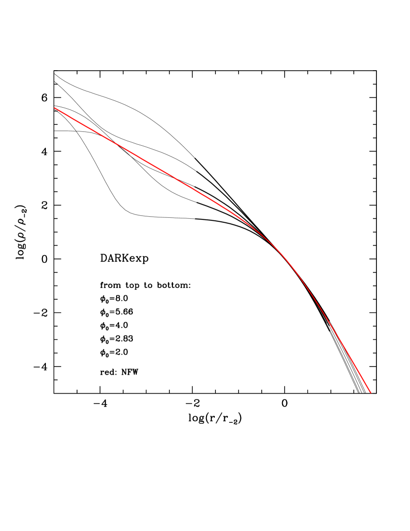
Figure 2: Density profiles of the five DARKexp models shown in Figure 1, normalized such that at the radius where the density slope $\gamma=2$, the density is unity. The radial range accessible to the highest resolution pure dark matter N-body simulations is highlighted as thick lines. The red line is the NFW model shown for reference.

Given a distribution function $f(E)$ one can integrate it over the velocity space to obtain the density distribution as a function of radius, $\rho(r)$. However, given a distribution in energy, $N(E)$ one cannot obtain $\rho(r)$ in one step. This is because unlike $f(E)$, $N(E)$ contains in it the density of states, and so it already depends on the potential, which is what one is trying to recover. Therefore an iterative procedure is needed, such as the one described in Binney (1982), which assumes isotropy. Since there is only one free parameter in DARKexp, $\phi_{0}$, the density profiles are a function of $\phi_{0}$ only; these are shown in Figure 1, where we plot the logarithmic density slope, $\log(\gamma)$, where $\gamma=-d\log(\rho)/d\log(r)$. The concept of ‘virial radius’ is not defined in these systems, so we chose to normalize the radius to that where the density attains $\gamma=2$, and call it $r_{-2}$. The blue line is the Navarro et al. (2004) $\alpha=0.17$ model, while the two red lines are the NFW (Navarro et al., 1997), and the Hernquist (Hernquist, 1990) profiles, shown for reference. The corresponding density profiles are plotted in Figure 2; thick lines highlight the radial range accessible to high-resolution numerical simulations (Navarro et al., 2004; Stadel et al., 2009). The red curve is the NFW profile, shown for comparison.

The DARKexp family of density profiles has a characteristic shape. At radii larger than $\sim 0.01\;r_{-2}$, i.e. those that can be probed in simulated systems, and for small values of $\phi_{0}$ the density profiles get shallower monotonically from large to small radii, but for $\phi_{0}$ above $\sim 4$ the profiles first get shallower until they reach $\gamma\approx 2$, then stay around $2$ for a finite radial range before becoming shallow again. This type of non-monotonic slope behavior is known to occur in some analytical systems, for example, the isothermal sphere (Binney & Tremaine (1987), Section 4.4, Figure 4.8), polytropic systems with index $n$ around 5 (Medvedev & Rybicki, 2001), and systems where $\rho/\sigma^{3}$ is a power law in radius (Austin et al., 2005). In the case of DARKexp, the slope of 2 is ‘inherited’ from the pure exponential $N(\varepsilon)=N_{0}\exp(-\beta\varepsilon)$ studied by Binney (1982).

Paper I demonstrated analytically that DARKexp models must asymptote to a central density cusp of $\gamma=1$. Figures 1 and 2 show that inside of $\sim 0.1-0.01\;r_{-2}$  DARKexp density profiles undergo oscillations in slope. Though the amplitude of oscillations can be large, especially for systems with shallow potentials, they bracket the slope of 1. More significantly, because these oscillations involve very little mass and take place in a narrow linear radial interval, any physical system, such as an N-body halo, which exhibits slight deviations from spherical symmetry or has a small amount of substructure, would erase these oscillations, averaging them to the asymptotic slope. In other words, because the amount of mass involved is small, the difference between the differential energy distribution of oscillating and a similar, but non-oscillating system will be small. (We note that some numerically generated systems do show small oscillations, see for example, Figure 2 of Stadel et al. (2009) and Figure 7 of Ludlow et al. (2010).)

The DARKexp systems that happen to have the smallest oscillations, even before the smearing effect of ellipticity or substructure is considered, are those with $\phi_{0}$ around 4, and so the asymptotic slope is already evident at radii somewhat interior to $r_{-2}$. Curiously, DARKexp models that most resemble N-body profiles are also those with $\phi_{0}\approx 4$ (compare to the red NFW and Hernquist profiles, and the blue Einasto, or Navarro et al. (2004) profiles, in Figure 1).

3 Testing DARKexp predictions

3.1 Choosing the appropriate numerical scheme

Because DARKexp makes a definite, one-parameter prediction about the shape of the energy distribution of isotropic systems, and because the corresponding density profiles have a distinct shape, the DARKexp model can be tested, using an appropriate numerical scheme. The scheme should satisfy certain criteria.

1. It should evolve a self-gravitating system collisionlessly.

2. To ensure that the statistical nature of the DARKexp is fulfilled each particle must undergo numerous interactions (with the potential) during relaxation.

3. It should allow unimpeded energy exchange between the particles and the potential.

4. It should not allow the exchange of angular momentum, or $J^{2}$, because DARKexp does not treat the redistribution of $J^{2}$, and it is possible, at least in principle, that in the process of redistributing $J^{2}$, the energy distribution will also be affected.

5. The final halos should be close to isotropic.

The first two criteria are satisfied by the collisionless dark matter N-body simulations, and the fifth one can be fulfilled by selecting nearly isotropic systems from the entire set of virialized halos. In fact, most simulated halos are close to isotropic, except for the outermost radii. The third criterion is probably satisfied, but the fourth is not satisfied by standard N-body simulations, because they have tangential forces and hence allow transfer of angular momentum. For example, formation of bar-like structures or central triaxiality is common in simulations (Merritt & Aguilar, 1985; Bellovary et al., 2008), and these tend to transfer angular momentum from the inner to the outer halo. A numerical scheme that does satisfy the fourth criterion is the extended secondary infall model, or ESIM, described in detail in Williams et al. (2004) and Austin et al. (2005) and summarized below.

3.2 Extended Secondary Infall Model

ESIM is a geometrically spherically symmetric shell code, where each shells’ angular and radial actions are held constant throughout the collapse. The initial conditions, detailed below, need not be cosmological, because the relaxation principles we are investigating are general, and do not hinge on cosmology. The only shell property that is allowed to change during evolution is its energy. ESIM does not calculate forces, instead, at every time step it recalculates each shell’s energy, i.e., solves the equation, $E=\Phi(r)+\frac{1}{2}\Bigl{[}v_{t}^{2}(r)+v_{r}^{2}(r)\Bigr{]}$ so that it agrees with the halo’s potential, which is the sum of the contributions of all the individual shells. Thus, energy redistribution in a collisionless fashion is allowed, while angular momentum redistribution is not, thereby fulfilling criterion (4) of DARKexp models.

A proto-halo is divided into concentric shells; the collapse proceeds inside-out with the innermost shell detaching from the Hubble flow first, reaching turn-around and collapsing. The second shell follows, etc. until some final epoch is reached. As each of the hundreds of shells reaches turn-around and collapses, the potential changes and so the energies of all the interior shells have to be readjusted to satisfy the energy equation. This repeated shell energy readjustment is what satisfies criterion (2) of Section 3.1. We note that unlike many analytical secondary infall models, the ESIM collapse factor, i.e., the ratio between the turn-around radius and the final equilibrium radius for a given shell is not pre-set; the shell finds its apocenter and pericenter that satisfy the energy equation.

There are two types of input for ESIM: the density profile for the initial proto-halo at an early epoch, and the rms of the random velocity dispersions. In the original Ryden & Gunn (1987) prescription the density profile shape function is taken from Bond et al. (1986), and depends on the matter power spectrum, $P(k)$. The rms of the random velocities are calculated based on $P(k)$.

In this paper the two types of inputs are not derived from a cosmological $P(k)$. For a given shell the magnitude of the random velocity is picked randomly from a Maxwellian distribution having the specified rms, and the splitting between radial and tangential directions is done randomly. These random velocity components are imparted to the shell at turn-around, $r_{to}$. The tangential component gives the shell’s angular momentum per unit mass, $J=v_{tan}r_{to}$, and the radial component is added to the radial velocity developed through collapse.

To test DARKexp, we need nearly isotropic systems. ESIM halo evolution drives halos toward isotropy, but full isotropy usually cannot be achieved, because of the constraint that all shells keep their $J$’s fixed. To satisfy criterion (4) of Section 3.1 we generate a large number of halos by varying the two initial conditions, the density and rms velocity dispersion profiles of proto-halos, evolving them, and then selecting the final halos that are close to isotropic. We did not try to generate systems that would resemble N-body halos (or have $\phi_{0}$ near 4), instead we wanted our halos to span the broadest range of DARKexp profile behavior.

We use five ESIM halos; their initial conditions are shown in Figure 3. The top panel has the density profiles, while the bottom has the angular momentum distribution, $J(r)$. The density profiles represented by the long and short dashed lines in the upper panel correspond to $J(r)$ distributions of the same line type. The solid line density profile was evolved using three different $J(r)$’s represented by solid lines in the bottom panel. Three of the initial $J(r)$ profiles (long dashed, short dashed, and one of the solid lines) follow the original Ryden & Gunn (1987) prescription, while the remaining two solid line $J(r)$’s are modified to generate intermediate values of $\phi_{0}$ in the final halos.

Before we proceed, we point out that most physical collapse and relaxation schemes designed to test DARKexp predictions will be limited to some degree. The limitations of N-body simulations were already pointed out. In ESIM, it is impossible to strictly comply with criteria (3) and (4) of Section 3.1 simultaneously. Since the halos are not allowed to redistribute their angular momentum among shells, this indirectly imposes restrictions on how well the energy can be redistributed. For example, a shell which was endowed with a large $J$ as its initial condition cannot come close to the halo center, and thus cannot have energy arbitrarily close to $\phi_{0}$. Consequently, energy cannot be redistributed completely freely, and condition (3) may not be fully satisfied in all halos.

3.3 Energy distributions

Figure 4 shows the energy distributions of five evolved ESIM halos described above. Each halo was fit with DARKexp $N(\varepsilon)$, with two free parameters, the normalization and temperature, $T=1/\beta$, and the fits are shown as curves. The normalization parameter is related to the total mass of the halo, and is irrelevant here. In the Figure the normalization was set arbitrarily, to space out the curves evenly. The only relevant parameter is $\beta$. The fitting is done over the energy range $E_{max}$ to $E_{t}$, where $E_{max}$ is the energy of the most bound shell, and $E_{t}$ is the energy where ESIM halos begin to deviate from a straight line in the $\log[N(E)]$ vs. $E$ plot. This choice is somewhat, but not too arbitrary; Figure 4 shows that for any given halo the deviation starts relatively abruptly. For plotting purposes, the energy scale of each halo was multiplied by $\beta$, so the horizontal axis is in dimensionless units of $\beta(|E_{max}|-|E|)=\phi_{0}-\varepsilon$, and $\beta$ is different for each halo.

It is apparent that ESIM energy distributions are very well fit by DARKexp. The deviations are seen at large $\phi_{0}-\varepsilon$, i.e., for loosely bound shells which inhabit the outer, not yet equilibrated portions of halos. For most ESIM halos the DARKexp fit is valid for a wide enough range of energies and $N(\varepsilon)$, so that the best-fitting function is, unmistakably, $N(\varepsilon)\propto[\exp(\phi_{0}-\varepsilon)-1]$.

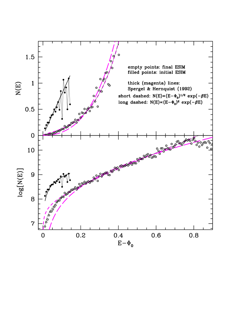
Figure 5: The $\phi_{0}=6.5$ ESIM halo of Figure 4. The top panel has a linear vertical scale, while the bottom panel, log. The filled points are the initial, pre-collapse energy distribution, and the empty points are the final. (Vertical normalization is arbitrary.) Note that the initial energy distribution is narrow, has a shallower $\Phi_{0}$ than the final distribution, and is roughly linear in energy. The two thick magenta lines represent the two extreme cases of the Spergel & Hernquist (1992) model, as labeled in the plot.

To illustrate this point we compare in Figure 5 the $\phi_{0}=6.5$ ESIM halo (empty points) from Figure 4 to the prediction of the scattering model proposed by Spergel & Hernquist (1992). Their $N(E)$ goes approximately as $[(E-\Phi_{0})^{-2}+C(E-\Phi_{0})^{-1/2}]^{-1}\exp(-\beta E)$. The two extremes of this function are shown as the short dashed (magenta) line in the limit where $N(E)=(E-\Phi_{0})^{1/2}\exp(-\beta E)$, and long dashed (magenta) line in the limit where $N(E)=(E-\Phi_{0})^{2}\exp(-\beta E)$. Both fail to match ESIM halos.

We also compare DARKexp to another physically motivated model of halo formation. Non-extensive statistical mechanics (Tsallis, 1988) predict collisionless systems to be polytropes (Plastine & Plastino, 1993), which have distribution functions that are power laws in energy, with a cutoff at the most bound energy (Binney & Tremaine (1987), eq. 4-105). The distribution function of the central regions of DARKexp is also a truncated power law (Paper I, eq. 21), but the exponent is $n=-1$, while polytropes have $n>1/2$. In the outer regions both polytropes and DARKexp density profiles are approximately power laws in radius, but the transition between the inner and outer slope is much faster in polytropes than in the DARKexp systems. Overall, DARKexp is quite different from polytropes.

Note that the initial, pre-collapse shape of the ESIM energy distribution is very different from the final, so the goodness of the DARKexp fit is not the result of (un)luckily chosen initial conditions. The filled points in Figure 5 show the initial energy distribution of the $\phi_{0}=6.5$  ESIM halo. It is much narrower than the final distribution and is linear in energy; also the potential depth of the pre-collapse halo, $\Phi_{0}$, is considerably shallower than that of the final. The initial conditions of the other four halos are similar.

Because ESIM is a shell code with the proto-halo shell thickness increasing outward logarithmically, the mass resolution is considerably better in the inner regions than in the outer. The portions of the energy distribution histogram with energies near most bound typically have a few hundred (relatively low mass) shells in each bin, so the region in $N(\varepsilon)$ which matters most for comparison with DARKexp has the highest resolution. This is not so for N-body codes, where each particle has equal mass. The inset in Figure 4 shows that near the most bound energies the distribution is linear, as is expected from DARKexp, $N(\varepsilon)=\exp(\phi_{0}-\varepsilon)-1\approx 1+(\phi_{0}-\varepsilon)+(\phi_{0}-\varepsilon)^{2}/2+...-1\approx(\phi-\varepsilon)$.

3.4 Density, velocity dispersion, and $\rho/\sigma^{3}$ profiles

In addition to the energy distribution, one can also do the comparison with the density and velocity distributions. Because DARKexp $N(\varepsilon)$ is dimensionless (for example, the virial radius, $r_{200}$ has no meaning in DARKexp), and ESIM quantities are dimensional ($r_{200}$ is clearly defined), we first have to put these on the same footing. To that end, we estimate the dimensionless potential depth $\phi_{0}$ for each ESIM halo using $\phi_{0}=\beta(|E_{max}|-|E_{min}|)$, where $E_{min}$ is the energy of the least bound shell. What energy represents the least bound shell is not clear; potential differences are readily known, but not absolute potential values. We estimate $|E_{min}|$ as $|E_{200}+E_{t}|/2$, where $E_{200}$ is the typical energy of particles at the radius where the average interior density is 200 times the critical, and $E_{t}$ is defined in Section 3.3. Note that $|E_{200}|$ is always less than $|E_{t}|$, implying that ESIM halos are not equilibrated up to the virial radius.

Given this estimate of $\phi_{0}$, we can check how well the ESIM density profiles reproduce the corresponding DARKexp $\rho(r)$. The two should match reasonably well, but perfect agreement is not expected because (i) some ESIM halos do not follow DARKexp $N(\varepsilon)$ for a wide energy range (see Section 3.2), (ii) estimating $E_{min}$ is not rigorous, and (iii) none of the ESIM halos are perfectly isotropic. All five halos are shown in Figure 6, against the background of DARKexp models with $\phi_{0}$ values from 2 to 10, in steps of 0.5; the ones fitting the five ESIM halos are shown as thicker lines. As for $N(\varepsilon)$, the DARKexp models provide very good fits to most of the ESIM halo density profiles. ESIM halos with the shallower potentials do not match DARKexp predictions as well as the ones with deeper potentials. This could be because the shallower halos do not undergo as much change in the potential during the evolution, and hence do not relax fully.

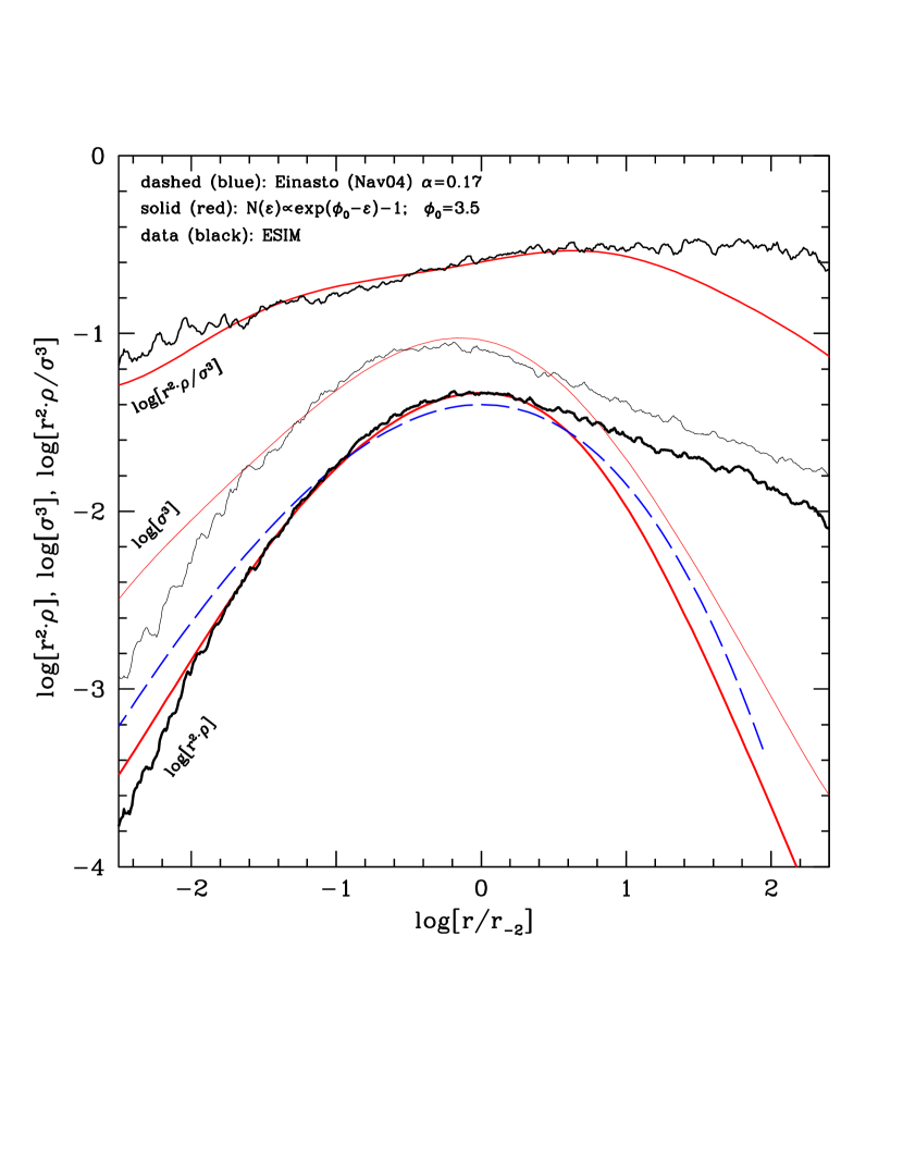
Figure 8: Same as Figure 7, but for the ESIM and the corresponding DARKexp halo with $\phi_{0}=3.5$. Note that here the ESIM density and the velocity dispersion profiles deviate from DARKexp, possibly because the former is not fully relaxed owing its shallow potential. ESIM $\rho/\sigma^{3}$ remains a power-law.

The second ($\phi_{0}=6.5$) and the fourth ($\phi_{0}=3.5$) of the five profiles of Figure 4 are shown in Figures 7 and 8, where we plot $\log(\rho\cdot r^{2})$ of the ESIM halos (black lines with ’noise’), and the best-fitting DARKexp curve (red smooth lines). The radii are in units of $r_{-2}$, but the vertical normalization is arbitrary, so only the shapes of the curves are to be compared. The halo with the deeper potential (Figure 7) closely follows the DARKexp prediction for nearly four decades in radius, whereas the shallower one, does so for only two decades, and deviations become pronounced in the outer halo. We note that these density profile shapes, especially for the deeper potentials, like in Figure 7, where the density slope stays roughly constant for a finite radial range were already evident in Figure 1 of Williams et al. (2004).

We use the isotropic Jeans equation to obtain the velocity dispersion profile for each halo, shown as thin lines in Figures 7 and 8. Note that the DARKexp  $\sigma^{3}$ shape tracks the density profiles shape, ensuring that $\rho/\sigma^{3}$ (the top smooth line) stays close to a power law for $\sim 3$ decades in radius. The reason for the pseudo phase-space density, $\rho/\sigma^{3}$ being a power law in collisionless simulations is still not known, but it is reassuring that DARKexp models predict this feature.

In Figure 7, while the ESIM density profile is very well fit by DARKexp, the shape of the velocity dispersion profile, $\sigma^{3}$, which we define as $\sigma_{rad}\sigma_{\theta}\sigma_{\phi}=\sigma_{rad}\sigma_{tan}^{2}=\sigma_{rad}^{3}[1-\beta(r)]$, deviates from DARKexp predictions because of ESIM’s non-zero anisotropy, $\beta(r)$. The top set of curves shows $\rho/\sigma^{3}$, which also deviate somewhat from DARKexp predictions, again, because of anisotropy.

4 Conclusions

Because the sole dynamical action of the ESIM is to repeatedly readjust shells’ energies in response to the changing potential, it is well suited for testing the DARKexp predictions described in Paper I (Hjorth & Williams, 2010). This constant reshuffling of energies drives halos to the most probable, DARKexp state. The more realistic numerical schemes, like the N-body simulations are also more complex in the sense that they do more than just redistribute particle energies, they also affect the redistribution of angular momentum. Whether the inclusion of this additional degree of freedom will preserve the DARKexp $N(\varepsilon)$ form is not yet clear. We speculate that the changes, at least in the inner portions of halos will be minor because N-body halos are fully relaxed and isotropic in those regions.

The argument presented in Paper I does not rely on any specific process, like infalling substructure or dynamical friction, to achieve the final state; it is a maximum entropy argument. If the same principle applies to the redistribution of angular momentum in collisionless simulations of dark matter halos, then the final $N(E,J^{2})$ distribution can also be arrived at similarly, without knowing the details of the radial orbit, or other tangential instabilities that operate in simulations. Encouraged by the success of our isotropic investigations we will pursue the statistical mechanical approach, and apply it to anisotropic systems.

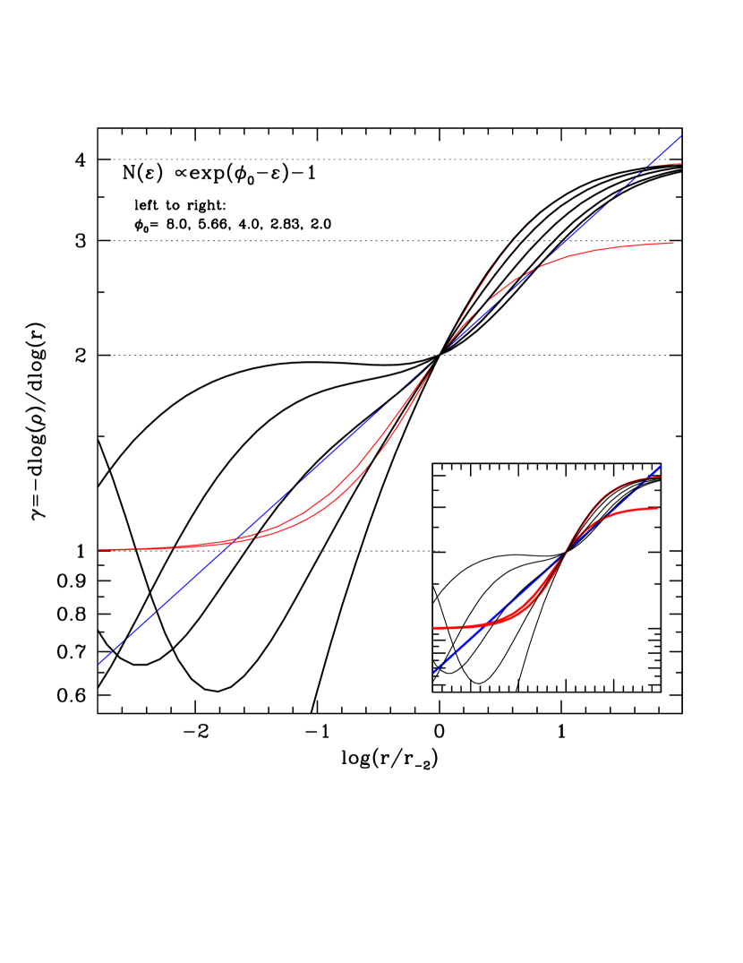
Figure 1: Density profile slopes predicted by the isotropic DARKexp model (thick black lines). From left to right the halo potential depths are $\phi_{0}=8.0,5.66,4.0,2.83,2.0$. These five values span the range of typical behavior, and are spaced equally in log. Note that the vertical scale is logarithmic, because the Navarro et al. (2004) fits to N-body halos (Einasto profiles) are straight lines in this representation; $\alpha=0.17$ profile of Navarro et al. (2004) is plotted as a straight blue line. The two red curves are the Hernquist and NFW profiles (NFW asymptotes to the outer slope of 3) shown for reference. The horizontal axis is normalized to the radius, $r_{-2}$, where the density slope attains $\gamma=2$. The inset is the same as the main figure, but plots DARKexp as thin lines so that the other three profiles are more visible.

Figure 3: Initial density profiles and angular momentum distributions for the five ESIM halos. In the upper panel the profile are labeled by the final $\phi_{0}$. The initial density profile shown with the solid line was evolved using three different initial angular momenta profiles (all shown with the solid line in the bottom panel). The density profiles represented by the long and short dashed lines in the upper panel correspond to $J(r)$ distributions of the same line type in the lower panel. The short vertical line segments in the upper panel indicate roughly the radial range shown in Figures 6-8.

Figure 4: Differential energy distribution of five ESIM halos. The thin lines are the best fit DARKexp models, fit up to the energy where ESIM halos begin to clearly deviate form exponential. The inverse temperature, $\beta$, and the dimensionless potential depth, $\phi_{0}$ for each halo are shown in the plot. The inset is a linear plot of the most bound portions of the five halos, up to $\phi_{0}-\varepsilon\sim 1$. The vertical scale has been rescaled so that all the DARKexp fits coincide, and are shown as the single line in the inset. Note that the most bound portions of ESIM halos have linear $N(\varepsilon)$.

Figure 6: Similar to Figure 1, but with five ESIM halos superimposed. The corresponding DARKexp models are highlighted as thick lines; the rest of DARKexp models (from $\phi_{0}=2$ to 10, in steps of $0.5$) are shown as thin dotted lines. Compared to Figure 1, in this Figure we spaced out the curves horizontally, to avoid overcrowding.

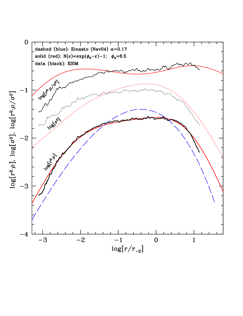
Figure 7: Density, velocity dispersion, and pseudo phase-space density of the ESIM (black) and the corresponding DARKexp halo (red), with $\phi_{0}=6.5$ plotted in Figure 4. The lowest two curves (thick lines) are the density profiles, multiplied by $r^{2}$. The DARKexp is an excellent fit to ESIM over 4 decades in radius. The dashed line is the Einasto (or, Navarro et al. (2004)), shown for comparison. The middle two curves (thin lines) are: $\sigma^{3}$ for the isotropic DARKexp models, and $\sigma^{3}=\sigma_{rad}\sigma_{tan}^{2}$ for ESIM, which are not exactly isotropic. The difference between ESIM and DARKexp velocity dispersion profiles are due to ESIM halo anisotropy. This difference is also reflected in the top set of two curves, $r^{2}\cdot(\rho/\sigma^{3})$. The vertical normalization of curves is arbitrary.

References

- Austin et al. (2005) Austin C.G., Williams L.L.R., Barnes E.I., Babul A. & Dalcanton, J.J. 2005, ApJ, 634, 756
- Bellovary et al. (2008) Bellovary, J. M., Dalcanton, J. J., Babul, A., Quinn, T. R., Maas, R. W., Austin, C. G.,Williams, L. L. R., Barnes, E. I. 2008, ApJ, 685, 739
- Bond et al. (1986) Bond, R., Bardeen, J., Kaiser, N. & Szalay, A. 1986, ApJ
- Binney (1982) Binney, J. 1982, MNRAS, 200, 951
- Binney & Tremaine (1987) Binney, J. & Tremaine, S. 1987, Galactic Dynamics, Princeton University Press, 1st edition
- Hernquist (1990) Hernquist, L. 1990, ApJ, 356, 359
- Hjorth & Madsen (1991) Hjorth, J. & Madsen, J. 1991, MNRAS, 253, 703
- Hjorth & Williams (2010) Hjorth, J. & Williams, L.L.R. 2010, ApJ, submitted (Paper I)
- Ludlow et al. (2010) Ludlow, A.D. et al. 2010, preprint, arXiv:1001.2310
- Lynden-Bell (1967) Lynden-Bell, D. 1967, MNRAS, 136, 101
- Madsen (1996) Madsen, J. 1996, MNRAS, 280, 1089
- Medvedev & Rybicki (2001) Medvedev, M.V. & Rybicki, G. 2001, ApJ, 555, 863
- Merritt & Aguilar (1985) Merritt, D., Aguilar, L. A. 1985, MNRAS, 217, 787
- Merritt et al. (1989) Merritt, D., Tremaine, S. & Johnstone, D. 1989, MNRAS, 236, 829
- Navarro et al. (1997) Navarro, J.F., Frenk, C.S. & White, S.D.M. 1997, ApJ, 490, 493
- Navarro et al. (2004) Navarro, J.F. et al. 2004, MNRAS, 349, 1039
- Plastine & Plastino (1993) Plastino, A.R. & Plastino, A. 1993, Phys. Lett. A, 174, 384
- Ryden & Gunn (1987) Ryden, B.S. & Gunn, J.E. 1987, ApJ, 318, 15
- Spergel & Hernquist (1992) Spergel, D.N. & Hernquist, L. 1982, ApJ, 397, L75
- Stadel et al. (2009) Stadel, J., Potter, D., Moore, B., Diemand, J., Madau, P., Zemp, M., Kuhlen, M. & Quilis, V. 2009, MNRAS, 398, L21
- Stiavelli & Bertin (1987) Stiavelli, M. & Bertin, G. 1987, MNRAS, 229, 61
- Tsallis (1988) Tsallis, C. 1988, J. Stat. Phys., 52, 479
- Williams et al. (2004) Williams, L.L.R., Babul, A. & Dalcanton, J.J. 2004, ApJ, 604, 18