Flow analysis with cumulants: direct calculations
Abstract
Anisotropic flow measurements in heavy-ion collisions provide important information on the properties of hot and dense matter. These measurements are based on analysis of azimuthal correlations and might be biased by contributions from correlations that are not related to the initial geometry, so called non-flow. To improve anisotropic flow measurements advanced methods based on multi-particle correlations (cumulants) have been developed to suppress non-flow contribution. These multi-particle correlations can be calculated by looping over all possible multiplets, however this quickly becomes prohibitively CPU intensive. Therefore, the most used technique for cumulant calculations is based on generating functions. This method involves approximations, and has its own biases, which complicates the interpretation of the results. In this paper we present a new exact method for direct calculations of multi-particle cumulants using moments of the flow vectors.
pacs:
25.75.Ld, 25.75.Gz, 05.70.FhI Introduction
Anisotropic flow is a response of the system created in a heavy-ion collision to the anisotropies in the initial geometry. Thus, anisotropic flow is very sensitive to the properties of the system at an early time of its evolution. The sizable azimuthal momentum-space anisotropy observed at RHIC energies (for a review, see Voloshin:2008dg ; Sorensen:2009cz ) is the main evidence for the nearly perfect liquid behavior Teaney:2009qa ; Heinz:2009xj of the created matter. Quantitatively, anisotropic flow is characterized by coefficients in the Fourier expansion of the azimuthal dependence of the invariant yield of particles relative to the reaction plane Voloshin:1994mz ; Poskanzer:1998yz :
| (1) |
Here is the energy of particle, is the transverse momentum, is its azimuthal angle, is the rapidity, and the reaction plane angle (see Fig 1). The first coefficient, , is usually called directed flow, and the second coefficient, , is called elliptic flow. In general the coefficients are and dependent – in this context we refer to them as differential flow. The integrated flow is defined as a weighted average with the invariant distribution used as a weight:
| (2) |
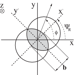
Since the reaction plane is not known experimentally, the anisotropic flow is estimated using azimuthal correlations between the observed particles. For example, using 2-particle azimuthal correlations:
| (3) |
where the first term, , is the part due to anisotropic flow, and represents the so called non-flow contribution, that comes from correlations not related to the initial system geometry. If non-flow is small, Eq. (3) can be used to measure , but in general the non-flow contribution is not negligible. To suppress non-flow one can exploit the collective nature of anisotropic flow using multi-particle correlations. The method based on multi-particle cumulants (genuine multi-particle correlations) to measure anisotropic flow was proposed in Borghini:2000sa ; Borghini:2001vi ; Borghini:2001zr ; Adler:2002pu . This method allows to subtract non-flow effects from flow measurements order by order. Note that some experimental artifacts, such as track splitting, in the analysis also contribute to the two particle correlation; in this respect multi-particle techniques are also valuable, as they suppress such contributions as well.
One of the problems in using multi-particle correlations is the computing power needed to go over all possible particle multiplets, which practically prohibits calculations of correlations of order larger than (three-particle correlations). To avoid this problem, it was suggested in Borghini:2000sa to express cumulants in terms of moments of the magnitude of the corresponding flow vector , defined as:
| (4) |
where is the number of particles. Unfortunately, flow estimates from cumulants constructed in such a way were systematically biased by the interference between various harmonics. An improved cumulant method using the formalism of generating functions suggested in Borghini:2001vi ; Borghini:2001zr fixed the problem of interfering harmonics while keeping the number of operations still linear with multiplicity . For this approach the analytical calculations become rather tedious and therefore the solutions are obtained using interpolation formulae. Unfortunately this introduces numerical uncertainties and requires tuning of interpolating parameters for different values of the flow harmonics and multiplicity. More recently a Lee-Yang-Zero’s sum method BBO:2003a ; Bhalerao:2003xf ; Borghini:2004ke ; Bilandzic:2008nx has been developed to suppress non-flow contribution to all orders. Closely related to that are methods of Fourier and Bessel transforms of the -distributions Voloshin:2006gz , and the method of direct fitting of the -distribution. All these methods, while indeed being almost insensitive to non-flow, are biased by interference of different harmonics.
In this paper we present a new method to calculate multi-particle cumulants in terms of moments of (in general, different harmonics) -vectors. In our approach the cumulants are not biased by interference between various harmonics, interpolating formulas used in the formalism of generating functions are not needed, and, moreover, all detector effects can be disentangled from the flow estimates in a single pass over the data at the level of or better than any other method. The number of operations required in our approach is still for each . Since in our approach cumulants are calculated without any approximation and directly from the data we often call them direct cumulants (also referred to as -cumulants because they are expressed analytically in terms of different harmonic -vectors).
Flow fluctuations are an important part of an anisotropic flow study. It is believed that flow fluctuations are mostly determined by initial geometry fluctuations Miller:2003kd of the system created in a collision. An important consequence of this is that the anisotropic flow develops relative to the so-called participant plane(s) instead of the reaction plane determined by the direction of the impact parameter Manly:2005zy . We note that the method to calculate cumulants proposed in this paper is not influenced by how exactly the anisotropic flow is being developed.
In our simulations we show results obtained up to the 8-th order cumulant, although we think that in practice there is little advantage to go higher than order six, because going to higher order does not remove the systematic uncertainty related to contribution from clusters exhibiting flow (see the discussion of systematic uncertainties associated with cumulant analysis in Adams:2003zg ). For example, in a 4-particle correlation analysis this bias corresponds to the situation when two particles are correlated because they are coming from the same cluster and, in addition, correlated with another two particles via flow.
The paper is organized as follows. After the main definitions are introduced in section II, we describe how the so-called reference flow can be calculated. The reference flow is an average flow in some momentum window; it is needed for the calculation of the differential flow of particles of interest. To optimize the procedure, the reference flow can be calculated using weights, e.g. weighted with transverse momentum of the particle. Thus the reference flow can be noticeably different from integrated flow of the same particles. Section IV describes how the differential flow is calculated. To show how the method works in different environments and how it compares to some other methods we show simulation results in section V. Finally, we summarize the main features of the method. Technical details, including the derivation of the main equations, equations in case of using non-unity weights in the calculation of reference flow, and acceptance effects are provided in Appendices.
II Multi-Particle azimuthal correlations and cumulants
In this paper we discuss mostly 2- and 4-particle azimuthal correlations (formulae for 6-particle correlation are provided in the Appendix), but the generalization to azimuthal correlations involving more particles is straightforward. The method can be easily applied for calculations of mixed harmonics multi-particle correlations. In fact, mixed harmonics correlations are needed in our approach for calculations of any multi-particle correlations with order higher than 2. Presenting 4-particle correlations below, we also show how the 3-particle correlations, involving one particle of a double harmonic can be calculated. All the correlations are obtained by first averaging over all particles in a given event and then averaging over all events. The latter may involve weights depending on event multiplicity.
We define single-event average 2- and 4-particle azimuthal correlations in the following way:
| (5) | |||||
| (6) | |||||
where , and the prime in the sum means that all indices in the sum must be taken different.
The second step involves averaging over all events:
| (7) | |||||
| (8) | |||||
where by double brackets we denote an average, first over all particles and then over all events. and are the event weights, which are used to minimize the effect of multiplicity variations in the event sample on the estimates of 2- and 4-particle correlations. In general, the optimal choice of weights would be determined by the multiplicity dependence of . The best approach might be to calculate the cumulants at fixed and then average over the entire event sample. In our calculations, with independent of multiplicity, we use:
| (9) | |||||
| (10) |
The above choice for the event weights takes into account the number of different 2- and 4-particle combinations in an event with multiplicity .
The general formalism of cumulants was introduced into flow analysis by Ollitrault et al Borghini:2000sa ; Borghini:2001vi ; Borghini:2001zr . We will use below the notations from those papers. The order cumulant, , is simply an average of 2-particle correlation defined in Eq. (7):
| (11) |
As was pointed out first in Borghini:2001vi the genuine -particle correlation (i.e. -particle cumulant), is given by:
| (12) |
Expressions (11) and (12) are applicable only for detectors with uniform acceptance and will be generalized in Appendix C to extend their applicability for detectors with non-uniform acceptance.
Different order cumulants provide independent estimates for the same reference harmonic . In particular Borghini:2001vi :
| (13) | |||||
| (14) |
where the notation is used to denote the reference flow estimated from the order cumulant , and stands for the reference flow estimated from the order cumulant .
III Reference flow
To obtain the order cumulant it suffices to separate diagonal and off-diagonal terms in :
| (15) |
which can be trivially solved to obtain :
| (16) |
The event averaging is being performed via Eq. (7). The resulting expression for is than used to estimate order cumulant (see Eq. (11)), which in turn is used to estimate the reference flow harmonic by making use of Eq. (13).
To obtain the order cumulant we start with the decomposition of (for details, see Appendix A)
| (17) |
We have four distinct cases for the indices , , and : 1) they are all different (4-particle correlation), 2) three are different, 3) two are different or 4) they are all the same. Note, that the case of three different indices corresponds to the so-called mixed harmonics 3-particle correlations, in many analyses of great interest by itself Adams:2003zg ; Borghini:2002vp . Equations for 3-particle correlations are provided in Appendix A. Taking everything into account, we obtain the following analytic result for the single-event average 4-particle correlation defined in Eq. (6):
| (18) | |||||
The reason why the originally proposed cumulant analysis Borghini:2000sa was biased lies in the fact that the terms consisting of -vectors evaluated in different harmonics (for instance terms and ) have been neglected. As seen from Eq. (18), such terms do appear in the analytic results and are crucial in disentangling the interference between harmonics. In particular, if a higher harmonic is present than picks up an additional contribution depending on that harmonic, namely , which is exactly canceled out with the contribution of harmonic to and , which read and , respectively.
The final, event averaged 4-particle azimuthal correlation, , is then obtained by making use of Eqs. (8) and (10). Using and one can calculate the order cumulant from Eq. (12).
The reference flow is mainly used to calculate differential flow. Therefore, one can optimize the calculation of reference flow to minimize the uncertainties in the final results. This is done by using different weights (e.g. particle transverse momentum) in the definition of flow vectors used in reference flow calculations. We provide all the equations necessary for calculations with weights in Appendix B.
The equations so far are applicable for an analysis with a detector with full uniform azimuthal coverage. In a non-ideal case one needs to take into account the acceptance corrections Bhalerao:2003xf ; Selyuzhenkov:2007zi . Acceptance affects the cumulants in three ways: (i) contributions from additional terms, e.g. proportional to or , that for a detector with full uniform azimuthal coverage are identical to zero, (ii) contributions from other flow harmonics, and (iii) the cumulant might be rescaled, which at the end can affect the final extracted flow values. We refer to Refs. Bhalerao:2003xf ; Selyuzhenkov:2007zi for a more complete discussion of acceptance effects. In practice the most important correction is the first one, for which we provide the full set of equations for a 2- and 4- particle cumulant analysis.
The generalized order cumulant which can also be used for detectors with non-uniform acceptance is:
| (19) | |||||
where for the last line we have used the fact that for instance and are the same quantities apart from the trivial relabeling. Remarkably, only two additional terms appear in Eq. (19), namely and , which counterbalance the bias to coming from very general detector inefficiencies. Further details on treating the acceptance effects, including formulae for the order cumulant are provided in Appendix C.
IV Differential flow
Once the reference flow has been estimated with the help of the formalism from previous section, we proceed to the calculation of differential flow. For that, all particles selected for flow analysis are labeled as Reference Flow Particle, RFP, and/or Particle Of Interest, POI. These labels are needed because flow analysis is being performed in two steps. In the first step one estimates the reference flow by using only the RFPs, while in the second step we estimate the differential flow of POIs with respect to the reference flow of the RFPs obtained in the first step.
IV.1 Reduced multi-particle azimuthal correlations
For reduced single-event average 2- and 4-particle azimuthal correlations we use the following notations and definitions:
| (20) | |||||
| (21) | |||||
where is the total number of particles labeled as POI (some of which might have been also labeled additionally as RFP), is the total number of particles labeled both as RFP and POI, is the total number of particles labeled as RFP (some of which might have been also labeled additionally as POI) in the event, is the azimuthal angle of the -th particle labeled as POI and taken from the phase window of interest (taken even if it was also additionally labeled as RFP), is the azimuthal angle of the -th particle labeled as RFP (taken even if it was also additionally labeled as POI). , as before, denotes the sum with all indices taken different.
Final, event averaged reduced 2- and 4-particle correlations are given by:
| (22) | |||||
| (23) |
In our calculations we use event weights and defined as:
| (24) | |||||
| (25) |
IV.2 Differential cumulants
We derive equations for the differential equations with the help of - and -vectors; the former built out of all POIs ( in total), and the second only from POI labeled also as RFP ( in total):
| (26) |
| (27) |
The -vector is introduced here in order to subtract effects of autocorrelations. Using those, we have obtained the following equations for the average reduced single- and all-event 2-particle correlations:
| (28) | |||||
| (29) |
For detectors with uniform azimuthal acceptance the differential order cumulant is given by
| (30) |
where, again we use notation from Ref. Borghini:2001vi . We present equations for the case of detectors with non-uniform acceptance in Appendix C.
Estimates of differential flow are being denoted as and are given by Borghini:2001vi :
| (31) |
Below we present the corresponding formulae for reduced 4-particle correlations:
| (32) | |||||
| (33) |
The order differential cumulant is given by Borghini:2001vi :
| (34) |
Equations for the case of detectors with non-uniform acceptance are again presented in Appendix C.
Having obtained estimates for and , we can estimate differential flow Borghini:2001vi :
| (35) |
Similarly to reference flow, we use the notation for differential flow harmonics obtained from order cumulants. and are independent estimates for the same differential flow harmonic .
V Simulation results
We have tested the new method with extensive simulations. The results, presented below, show that the method effectively suppresses non-flow contributions, illustrate the ability to remove the interference of the different harmonics, show the applicability for detectors having significant acceptance “holes”, and give an example of a differential flow analysis. In the figures, , shown in the first bin, represents the Monte Carlo estimate for , which was obtained using the known reaction plane event-by-event. Other estimates in the figures are obtained without using this information.
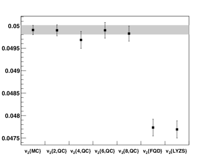
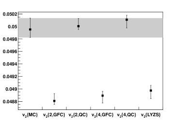
Figure 2 shows the results from a simulation of events with anisotropic flow present in two harmonics, the second and the fourth. Elliptic flow estimated by different methods is shown in the figure. A clear bias is observed in the estimates from fitting of the -distribution method and the Lee-Yang Zero’s Sum method, labeled as and , respectively. Results obtained with direct cumulants of different order, labeled as , are unaffected by interference.
(a)
(b)
(c)
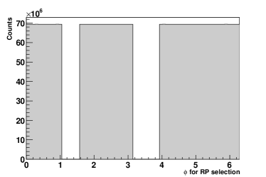
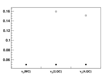
To demonstrate that the method works well even in cases with rather bad acceptance we simulated events with for a detector that had two large “holes” (see Fig. 3a). Figure 3b shows the obtained estimates using Eqs. (11) and (12) which are valid for detectors with perfect acceptance using open markers. Clearly these values are strongly biased. The estimates obtained from the more general equations for cumulants, namely Eqs. (66) and (71), which do account for the acceptance effects are shown as closed markers and agree with the Monte Carlo estimate. In Fig. 3c we look in more detail at the agreement with the Monte Carlo estimate and, in addition, compare to other methods.
The figure clearly shows that detector effects are corrected for at the level of or better than other methods.
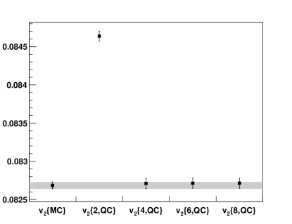
As an example of a differential flow analysis we show results for obtained with Therminator Kisiel:2005hn . As RFPs we select pions and as POIs we select protons. In the first step we estimate the reference flow by only making use of particles labeled as RFPs (using Eqs. (11), (12), (13) and (14)). The estimates of reference flow are presented in Fig. 4.
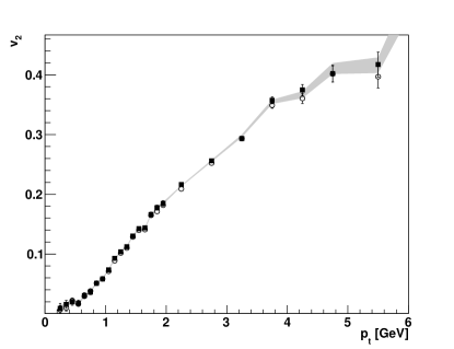
In the second step we estimate the differential flow of POIs (in this example protons were labeled as POIs) with respect to the reference flow of RFPs estimated in the first step. For each bin we evaluate and , and use equations (31) and (35) to estimate differential flow. The differential flow results for protons are presented in Fig. 5.
The resulting -integrated flow of protons calculated by making use of Eq. (2) is presented in Fig. 6.
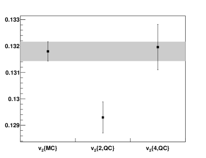
The figures for the integrated flow of the RFPs and POIs clearly show that the order cumulant is biased by nonflow while the higher order cumulants are in perfect agreement with the Monte Carlo.
VI Summary
In summary, we propose a new method to calculate multi-particle azimuthal correlations, which provides fast (in a single scan over the data) and exact (no approximations) non-biased (no interference between different harmonics) estimates for cumulants. In the paper, we provide the corresponding formulae for correlations up to the 6-th order, but the method, if needed, can be generalized for higher orders.
We have not discussed issues of the cumulant approach in general, such as multiplicity fluctuations, flow fluctuations, and low sensitivity for small flow values, but believe that our method will be helpful in investigating all these questions.
The proposed method has been extensively tested in simulations and has been used for real data analysis by the STAR and ALICE Collaborations Dhevan:PhD ; Ante:PhD . Further details about the method, including equations for 8-particle correlations, equations for estimates and evaluation of statistical errors, comparison to other methods, can be found in Ante:PhD .
Acknowledgements.
We thank Dhevan Gangadharan, Rene Kamermans, Naomi van der Kolk, Paul Kuijer, Mikolaj Krzewicki, Art Poskanzer, Gerard Smit, Paul Sorensen, Aihong Tang, Jim Thomas, Adam Trzupek, Fuqiang Wang and Evan Warren for their help, discussions, and interest in this work. The work of SV was supported in part by the US Department of Energy, Grant No. DE-FG02-92ER40713. The work of AB and RS was supported in part by the Dutch funding agencies FOM and NWO.Appendix A Equations for 3-, 4- and 6- particle correlations
Below we use the following definitions:
| (36) | |||||
| (37) | |||||
| (38) | |||||
| (39) | |||||
| (40) |
Using this notation one finds:
| (41) | |||||
The 2-particle correlations was already expressed in terms of the -vector evaluated in harmonic , see Eq. (16):
| (42) |
To obtain and we have to decompose
| (43) | |||||
and . After inserting results for and given in Eqs. (16) and (42), we arrive at the following equality:
| (44) | |||||
After inserting Eqs. (16), (42) and (44) into Eq. (41) and solving the resulting expression for the single-event average 4-particle correlations (Eq.(18)) follows.
This derivation can be generalized to obtain analytic results for any higher order multi-particle azimuthal correlations. Below we provide the expression for the 6-particle correlation:
| (45) | |||||
With that, the order cumulant is given by
| (46) |
and the reference flow is estimated as
| (47) |
Appendix B Particle weights
Below we provide formulae to use for the case when the reference flow is calculated using particle weights. For that we introduce a weighted -vector evaluated in harmonic :
| (48) |
where is a particle weight of the -th particle labeled as RFP and is the total number of RFPs in an event. In general, we will need flow vectors with power up to the order of multi-particle correlations. Similarly, we define
| (49) |
Note that only particles which have a RFP label, have a non-unit weight, while for the particles labeled as POI only, . For the subset of POIs which consists of all particles labeled both as POI and RFP ( in total) we introduce
| (50) |
For RFPs we also introduce:
| (51) | |||||
| (52) |
For all particles labeled both as RFP and POI we evaluate the following quantity:
| (53) |
while in the definition below the first sum runs over all POIs in the window of interest and the remaining sums run over all RPs in an event
| (54) |
Using the definitions presented above the weighted single-event 2- and 4-particle correlations are given by:
| (55) | |||||
| (56) |
The event weights (9) and (10) now read
| (57) | |||||
| (58) |
Analogously, the reduced single-event multi-particle correlations now read:
| (59) | |||||
| (60) |
where the event weights (24) and (25) are now:
| (61) |
The weighted average 2-particle correlations are given by the following equations:
| (62) | |||||
and the weighted average 4-particle correlations are given by:
| (63) |
where the weighted -vector, , was defined in Eq. (48) and in Eq. (51).
Appendix C Non-uniform acceptance
Building cumulants from multi-particle correlations we have so far omitted terms which vanish for the detectors with uniform acceptance. For a more general case they have to be kept Borghini:2000sa ; Borghini:2001vi ; Selyuzhenkov:2007zi ; K:1962 . The more general order cumulant now reads:
| (66) | |||||
The correction terms can be expressed in terms of the real and imaginary parts of the -vector (4):
| (67) | |||||
| (68) |
When particle weights are used the average 2-particle correlation is determined from Eqs. (62), while Eqs. (67) and (68) generalize into:
| (69) | |||||
| (70) |
where can be determined from the definition of the weighted -vector (48) and from definition (51).
The generalized order cumulant reads:
| (71) | |||||
The terms starting from the second line in Eq. (71) counter balance the bias coming from non-uniform acceptance so that is unbiased. These terms can be expressed in terms of -vectors:
| (72) | |||||
| (73) |
| (74) | |||||
| (75) | |||||
When particle weights are used the average 2-particle correlation is determined from Eqs. (62), the average 4-particle correlation is determined from Eqs. (63), the Eqs. (72) and (73) generalize into:
| (76) |
and the Eqs. (74) and (75) generalize into
| (77) |
The generalized order differential cumulant reads
| (78) |
Expressions for and were already given in Eqs. (67) and (68), respectively (when particle weights are being used in Eqs. (69) and (70), respectively). Similarly:
| (79) | |||||
| (80) |
where and were defined in Section IV. The Eqs. (79) and (80) remain unchanged when particle weights are being used.
The generalized order differential cumulant reads:
The terms starting from the second line in Eq. (C) counter balance the bias coming from non-uniform acceptance. Some of the new terms appearing in this expression can be expressed again in products of flow vectors:
| (82) |
When particle weights are used Eqs. (82) generalize into:
Eqs. (LABEL:3pAnizDFa) generalize into:
| (86) | |||||
and finally, Eqs. (LABEL:3pAnizDFb) generalize into:
| (87) | |||||
References
- (1) S. A. Voloshin, A. M. Poskanzer and R. Snellings, [arXiv:0809.2949].
- (2) P. Sorensen, [arXiv:0905.0174].
- (3) D. A. Teaney, arXiv:0905.2433 [nucl-th].
- (4) U. W. Heinz, [arXiv:0901.4355].
- (5) S. Voloshin and Y. Zhang, Z. Phys. C 70 (1996) 665 [arXiv:hep-ph/9407282].
- (6) A. M. Poskanzer and S. A. Voloshin Phys. Rev. C 58 (1998) 1671 [arXiv:nucl-ex/9805001].
- (7) N. Borghini, P. M. Dinh and J. Y. Ollitrault, Phys. Rev. C 63 (2001) 054906 [arXiv:nucl-th/0007063].
- (8) N. Borghini, P. M. Dinh and J. Y. Ollitrault, Phys. Rev. C 64 (2001) 054901 [arXiv:nucl-th/0105040].
- (9) N. Borghini, P. M. Dinh and J. Y. Ollitrault, [arXiv:nucl-ex/0110016].
- (10) C. Adler et al. [STAR Collaboration], Phys. Rev. C 66, 034904 (2002) [arXiv:nucl-ex/0206001].
- (11) R. S. Bhalerao, N. Borghini and J. Y. Ollitrault Phys. Lett. B 580, 157 (2004) [arXiv:nucl-th/0307018].
- (12) R. S. Bhalerao, N. Borghini and J. Y. Ollitrault Nucl. Phys. A 727 (2003) 373 [arXiv:nucl-th/0310016].
- (13) R. S. Bhalerao, N. Borghini and J. Y. Ollitrault J. Phys. G 30 (2004) S1213 [arXiv:nucl-th/0402053].
- (14) A. Bilandzic, N. van der Kolk, J. Y. Ollitrault and R. Snellings [arXiv:0801.3915].
- (15) S. A. Voloshin, arXiv:nucl-th/0606022.
- (16) M. Miller and R. Snellings, arXiv:nucl-ex/0312008.
- (17) S. Manly et al. [PHOBOS Collaboration], Nucl. Phys. A 774, 523 (2006) [arXiv:nucl-ex/0510031].
- (18) J. Adams et al. [STAR Collaboration], Phys. Rev. Lett. 92, 062301 (2004) [arXiv:nucl-ex/0310029].
- (19) N. Borghini, P. M. Dinh and J. Y. Ollitrault, Phys. Rev. C 66, 014905 (2002) [arXiv:nucl-th/0204017].
- (20) I. Selyuzhenkov and S. A. Voloshin Phys. Rev. C 77 (2008) 034904 [arXiv:0707.4672].
- (21) A. Kisiel, T. Taluc, W. Broniowski and W. Florkowski, Comput. Phys. Commun. 174, 669 (2006) [arXiv:nucl-th/0504047].
- (22) D. Gangadharan, Local Parity Violation in the Strong Interactions and Parton Collectivity in Au+Au Collisions at RHIC, Ph.D. thesis, University of California – Los Angeles, 2010.
- (23) A. Bilandzic, Ph.D. thesis (in preparation), Nikhef, Amsterdam, The Netherlands, 2011.
- (24) R. Kubo, Journal of the Physical Society of Japan, Vol. 17, No. 7, (1962).