Equilibrium distributions and relaxation times in gas-like economic models: an analytical derivation

Abstract

A step by step procedure to derive analytically the exact dynamical evolution equations of the probability density functions (PDF) of well known kinetic wealth exchange economic models is shown. This technique gives a dynamical insight into the evolution of the PDF, e.g., allowing the calculation of its relaxation times. Their equilibrium PDFs can also be calculated by finding its stationary solutions. This gives as a result an integro-differential equation, which can be solved analytically in some cases and numerically in others. This should provide some guidance into the type of probability density functions that can be derived from particular economic agent exchange rules, or for that matter, any other kinetic model of gases with particular collision physics.

I Introduction

The aim of mechanical statistics is to describe systems macroscopically based on the microscopic description of interactions of particles within the system. By defining the microscopic individual interaction of a collection of particles we can describe the system macroscopically by means of the Probability Density Function (PDF). A particular microscopic interaction will give rise to a definite PDF. And vice versa, a given PDF can come only from a small set of specific particle interactions. In this respect, the macroscopic PDF is also providing us with information about the microscopic interactions. A classical example is the Maxwell-Boltzmann distribution, which can be obtained as a solution of the Boltzmann integro-differential equation, which he proposed to explain the evolution of the PDF for a dilute gas.

Relatively recently, there has been growing interest in reproducing the PDF of money in a real economic system by molecular dynamics simulations Chakraborti and Chakrabarti (2000), Dragulescu and Yakovenko (2000), Chakraborti (2002), Hayes (2002), Chatterjee et al. (2004), Das and Yarlagadda (2005), López-Ruiz et al. (2009). In these statistical models, agents are allowed to exchange money following an exchange rule. PDFs from real economies follow Gibb’s exponential functions or Pareto’s laws Yakovenko (2009). Reproducing Gibb’s exponential functions with molecular dynamics simulations has proven simple by using a simple money exchange rule that conserves the total quantity of money Dragulescu and Yakovenko (2000). Pareto’s law distributions still remain a challenge, although some results do approximate it Levy et al. (1996),González-Estévez et al. (2008), Pellicer-Lostao and López-Ruiz (2010), Chakraborti and Manna (2010).

In this paper, we will show how to derive analytically the dynamical evolution equation of the PDF from the interaction rules of the agents. This process is very similar to the derivation of the Boltzmann integro-differential equation from the basic particle collision physics. Let us recall that this latter system has a Maxwell-Boltzmann PDF in equilibrium. Repetowicz et al. Repetowicz et al. (2005) have derived, by using mean-field approximation, the first moments of some of these economic models based on the formal solutions to the nonlinear Boltzmann equations derived by Ernst Ernst (1981). Lallouache et al. Lallouache et al. (2010) also calculate the moments of the random gas-like economic model with savings and its steady state solution. Düring et al. derive the moments of some economic models and their relaxation times Düring et al. (2008). We will demonstrate a simple step by step technique, different from the ones above, to derive the integro-differential equations of three economic models present in the reviews by Patriarca et al. Patriarca et al. (2010), Chatterjee and Chakrabarti Chatterjee and Chakrabarti (2007) or Yakovenko and Rosser Yakovenko and Jr. (2009). Some of these systems exhibit exponential PDFs as their steady state solutions. Other systems, which seem to follow Gamma distributions Patriarca et al. (2004) at their steady state, are in fact only approximated by them and do not follow them exactly Lallouache et al. (2010). We will show that some systems, in some particular cases, deviate appreciably from these Gamma distributions. We will derive the analytical formulas to calculate these distributions and we will compare these PDFs with Gamma distributions and molecular dynamics simulations. This technique should shed some light into the relationships between PDFs and the microscopic interactions of particles, and in particular, into the derivation of a Pareto type distribution from molecular dynamics simulations.

We also present, to our knowledge, for the first time, the dynamical equations of the evolution of the PDFs for these systems. This will allow us to study these systems not only from the point of view of their stationary PDFs, but also how they evolve in time. This area of research has often been neglected in the past, but it is key if we want to model the economy adequately by describing its evolution in time and not only in a static way. As an example, we will show how to derive the relaxation times of these systems.

II Pure random gas-like economic model

Figure 1: Dragulescu and Yakovenko’s economic model Dragulescu and Yakovenko (2000) which gives an exponential as the steady state PDF. Dots are the result of the molecular dynamics numerical simulations, and solid line is the exponential function which approximates the steady state PDF (Eq. 2). For these calculations, we take $<u>=1$.

We will introduce the technique directly with an example. In this case, we take the mapping introduced by Dragulescu and Yakovenko Dragulescu and Yakovenko (2000) to model the flow and distribution of money. This example is one of the simplest money exchange rules in which money is conserved in any transaction.

Assuming that we have $N$ agents trading with each other, the mapping that describes this statistical model is,

$$u^{\prime}_{i} = \epsilon\;(u_{i}+u_{j}),$$

$$u^{\prime}_{j} = (1-\epsilon)(u_{i}+u_{j}),$$

$$i,j = 1\ldots N,$$ (1)

where $\epsilon$ is a random generated number in the interval $(0,1)$, $u_{i}$ and $u_{j}$ are the initial money (or energy) and $u^{\prime}_{i}$ and $u^{\prime}_{j}$ are the final ones of agents $i$ and $j$, respectively, where the pair of agents $(i,j)$ is also randomly chosen for each transaction. These quantities, $u_{i}$, will always be positive. The steady state distribution, $f_{eq}$, obtained with numerical simulations of this system is shown in Fig. 1 (dotted line). It can be easily verified that it is an exponential or Gibbs distribution,

$$f_{eq}(u)=\beta\exp(-\beta u),$$ (2)

where $f(u){\mathrm{d}}u$ denotes the PDF, or probability of finding an agent with money (or energy) between $u$ and $u+{\mathrm{d}}u$. This PDF is normalized and the mean energy per particle then turns out to be

$$\langle u\rangle=\frac{1}{\beta}.$$ (3)

Let us now derive this function analytically. To do this, it is not only important the money exchange mapping (Eqs. II) in the determination of the PDF, but also the selection rule to choose which particles do interact at each time step. Therefore, we will explicitly describe the detailed and complete algorithm,

1. A pair of different agents are randomly selected in the system from a uniform distribution in the interval $[1,N]$. This is the pair $(i,j)$ in Eqs. II.

2. A random number $\epsilon$ between 0 and 1 is generated from a uniform distribution.

3. Exchange rules of Eqs. II are finally applied.

4. The application of all of the above “rules” will be denoted as a “step”. These steps are successively and indefinitely repeated.

We now derive the analytical expression for the PDF variation after each step, $\partial f(u)/\partial t$, for a given money $u$. Note that with this notation we assume that the time unit is one step. As explained in the next paragraphs in more detail, it can be straightforwardly seen that this variation comes on one side from the probability that agent $u$ has to be selected for a particular exchange, i.e., that $u_{i}$ or $u_{j}$ take the value $u$, and from another side from the probability that the result after the trading is $u$, i.e., that $u^{\prime}_{i}$ or $u^{\prime}_{j}$ give the value $u$. We can then write,

$$\frac{\partial f(u)}{\partial t} = \left[\frac{\partial f(u_{i})}{\partial t}+\frac{\partial f(u^{\prime}_{i})}{\partial t}\right.+$$ (4)

$$\left.\frac{\partial f(u_{j})}{\partial t}+\frac{\partial f(u^{\prime}_{j})}{\partial t}\right]_{u_{i}=u_{j}=u^{\prime}_{i}=u^{\prime}_{j}=u},$$

where all terms are maintained separated in the case that the trading rule is not symmetric in the indices $(i,j)$ before or after the interaction.

Let us see the detailed explanation for the present example. In rule 1, one particular agent from the whole population $N$ is selected. The probability that this particular agent is in the $[u_{i},u_{i}+{\mathrm{d}}u_{i}]$ range is proportional to the number of agents in that range, then the PDF for $u_{i}$ will be proportionally depleted by the quantity $f(u_{i}){\mathrm{d}}u_{i}$, that is,

$$\frac{\partial f(u_{i})}{\partial t}\sim-f(u_{i}).$$ (5)

Rule 1 will also deplete the PDF for $u_{j}$ in a similar way, that is, $\partial f(u_{j})/\partial t\sim-f(u_{j})$.

Rules 2 and 3 imply that, since $\epsilon$ is between 0 and 1, and according to Eqs. II, the net result verifies

$$0<u^{\prime}_{i}<u_{i}+u_{j},$$ (6)

where $u^{\prime}_{i}$ is equally distributed in the $[0,u_{i}+u_{j}]$ interval. This implies that the PDF for $u^{\prime}_{i}$ is increased proportionally to the number of agents with $u_{i}$ and $u_{j}$ and inversely to their total money $u_{i}+u_{j}$, that is, to the rate $f(u_{i}){\mathrm{d}}u_{i}f(u_{j}){\mathrm{d}}u_{j}/(u_{i}+u_{j})$. Then, the total variation $\partial f(u^{\prime}_{i})/\partial t$ will be obtained by integrating amongst all the possible values of $u_{i}$ and $u_{j}$ that give rise to the result $u^{\prime}_{i}$. In order to find the limits of integration in a simple way, we make a change of variables replacing $(u_{i},u_{j})$ by $(u_{i},U)$, where

$$U\equiv u_{i}+u_{j}.$$ (7)

Equation 6 is then transformed into $0<u^{\prime}_{i}<U$, which forces the integration limits of $U$ to be between $u^{\prime}_{i}$ and $\infty$. If $U$ is now fixed, and using its definition from Eq. 7, the integration limits of $u_{i}$ have to be between $0$ and $U$. With these new variables, the expression for $\partial f(u^{\prime}_{i})/\partial t$ is finally obtained

$$\frac{\partial f(u^{\prime}_{i})}{\partial t}\sim\int_{u^{\prime}_{i}}^{\infty}\mathrm{d}U\int_{0}^{U}\mathrm{d}u_{i}\frac{f(u_{i})f(U-u_{i})}{U}.$$ (8)

By symmetry of Eqs. II, a similar result for $\partial f(u^{\prime}_{j})/\partial t$ is just obtained by substituting $u^{\prime}_{i}$ for $u^{\prime}_{j}$ in Eq. 8.

As indicated by Eq. 4, to obtain the final result for a generic value $u$ we combine the decreasing term of Eq. 5 with the positive contribution of Eq. 8 to get

$$N\frac{\partial f(u)}{\partial t}=-2f(u)+2\int_{u}^{\infty}\mathrm{d}U\int_{0}^{U}\mathrm{d}u_{1}\frac{f(u_{1})f(U-u_{1})}{U},$$ (9)

where $N$ is the normalization factor for $\partial f(u)/\partial t$.

To derive the steady state solution we just set $\partial f(u)/\partial t=0$ to finally obtain

$$f_{eq}(u)=\int_{u}^{\infty}\mathrm{d}U\int_{0}^{U}\mathrm{d}u_{1}\frac{f_{eq}(u_{1})f_{eq}(U-u_{1})}{U}.$$ (10)

It is now easy to verify that the normalized exponential distribution from Eq. 2 satisfies this last equation. This analytical solution is plotted in Fig. 1, where it is verified that it is very much in agreement with the numerical simulations.

We shall now derive the relaxation time of this system. We will assume that we start with a PDF that is different from the equilibrium one (Eq. 2), but close to it. If we substitute this PDF into the right hand side of Eq. 10, we can verify (not shown here) that we obtain a very good approximation to the exponential equilibrium PDF (Eq. 2). The evolution equation close to the equilibrium is then simplified to,

$$N\frac{\partial f(u)}{\partial t}\simeq-2f(u)+2f_{eq}(u).$$ (11)

From here, we can immediately see that the relaxation time of the system is

$$\tau=\frac{N}{2}$$ (12)

collisions.

III Random gas-like economic model with saving

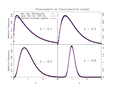
Figure 2: Chakraborti and Chakrabarti’s economic model Chakraborti and Chakrabarti (2000), which gives approximately a Gamma function as the steady state PDF, plotted for different values of the saving parameter, $\lambda$. Dots are the result of the molecular dynamics numerical simulations, blue solid line is the Gamma function which approximates the steady state PDF (Eq. 14) and red dashed line is the PDF which is the solution to the integro-differential equation 22. For these calculations, we take $<u>=1$.

We will now explore the gas-like economic model with saving introduced by Chakraborti and Chakrabarti Chakraborti and Chakrabarti (2000). The trading rules in this model are given by a random mapping that conserves the amount of money in each exchange, and in which each agent saves a fixed fraction, $\lambda$, of the money he owns before the transaction. More precisely, money is exchanged in the form,

$$u^{\prime}_{i} = \lambda\;u_{i}+\epsilon\;(1-\lambda)\;(u_{i}+u_{j}),$$

$$u^{\prime}_{j} = \lambda\;u_{j}+(1-\epsilon)\;(1-\lambda)\;(u_{i}+u_{j}),$$

$$i,j = 1\ldots N.$$ (13)

The steady state distribution obtained by numerical simulations of this system is shown in Fig. 2 (dotted lines). It is verified Patriarca et al. (2010) that it can be approximated by a Gamma distribution,

$$f_{eq}(u)\simeq au^{n-1}\exp\left(-nu/\langle u\rangle\right),$$ (14)

where $\langle u\rangle$ is the mean wealth of the multi-agent system, and $n$ is given by

$$n=\frac{1+2\lambda}{1-\lambda}.$$ (15)

The factor $a$ is found after the normalization of the PDF,

$$a=\frac{1}{\Gamma(n)}\left(\frac{n}{\langle u\rangle}\right)^{n}.$$ (16)

This Gamma function is plotted as a blue solid line in Fig. 2. It can be observed that it adjusts relatively well to the numerical simulations.

To derive the analytical expression of the steady state PDF we have to look at the precise rules for this mapping:

1. A pair of different agents of the system are randomly selected from a uniform distribution in the interval $[1,N]$. This will be the trading pair $(i,j)$ in Eqs. III.

2. A random number $\epsilon$ between 0 and 1 is generated from a uniform distribution.

3. The saving parameter $\lambda$ is maintained constant through the whole process.

4. Exchange rules of Eqs. III are finally applied.

5. The application of all of the above “rules” will be denoted as a “step”. These steps are successively and indefinitely repeated.

Let us derive now in an analytical way the PDF for this system. As in the previous model, rule 1 will deplete the density function $f(u)$ in $u_{i}$ by a quantity $\partial f(u_{i})/\partial t$ given by

$$\frac{\partial f(u_{i})}{\partial t}\sim-f(u_{i}),$$ (17)

and similarly, $\partial f(u_{j})/\partial t\sim-f(u_{j})$.

The mapping equations (Eqs. III) lead to the following inequalities

$$\lambda u_{i}<u^{\prime}_{i}<\lambda u_{i}+(1-\lambda)U,$$ (18)

where $u^{\prime}_{i}$, by using again $U=u_{i}+u_{j}$, is equally distributed in the $[\lambda u_{i},\lambda u_{i}+(1-\lambda)U]$ interval. This implies that the PDF for $u^{\prime}_{i}$ is increased proportionally to the number of agents with $u_{i}$ and $u_{j}$ and inversely to the length of the interval, $(1-\lambda)U$, where it is distributed, that is, to the rate $f(u_{i}){\mathrm{d}}u_{i}f(u_{j}){\mathrm{d}}u_{j}/((1-\lambda)U)$. Then, the total variation $\partial f(u^{\prime}_{i})/\partial t$ will be obtained by integrating amongst all the possible values of $u_{i}$ and $u_{j}$ able to give rise to the result $u^{\prime}_{i}$. The limits of integration can be easily found from Eq. 18:

$$u_{i} < u^{\prime}_{i}/\lambda,$$

$$u_{i} > (u^{\prime}_{i}-(1-\lambda)U)/\lambda$$ (19)

As in the former section for the Dragulescu and Yakovenko model Dragulescu and Yakovenko (2000), we obtain the result:

$$\frac{\partial f(u^{\prime}_{i})}{\partial t}\sim$$

$$\int_{u^{\prime}_{i}}^{\infty}\mathrm{d}U\int_{\max\left[\frac{u^{\prime}_{i}-(1-\lambda)U}{\lambda},\,0\right]}^{\min[u^{\prime}_{i}/\lambda,\,U]}\mathrm{d}u_{i}\frac{f(u_{i})f(U-u_{i})}{(1-\lambda)U}.$$ (20)

A similar formula can be derived for the $u^{\prime}_{j}$ variable. Combining these results (Eqs. 17 and III), the final expression for the PDF variation $\partial f(u)/\partial t$ in a generic value $u$ is derived:

$$N\frac{\partial f(u)}{\partial t}=$$

$$-2f(u)+$$

$$2\int_{u}^{\infty}\mathrm{d}U\int_{\max\left[\frac{u-(1-\lambda)U}{\lambda},0\right]}^{\min\left[u/\lambda,U\right]}\mathrm{d}u_{1}\frac{f(u_{1})f(U-u_{1})}{(1-\lambda)U},$$ (21)

where $N$ is again the normalization factor of $\partial f(u)/\partial t$.

To find the steady state solution, we just set $\partial f(u)/\partial t=0$ to finally get

$$f_{eq}(u)=\int_{u}^{\infty}\mathrm{d}U\int_{\max\left[\frac{u-(1-\lambda)U}{\lambda},0\right]}^{\min\left[u/\lambda,U\right]}\mathrm{d}u_{1}\frac{f_{eq}(u_{1})f_{eq}(U-u_{1})}{(1-\lambda)U}.$$ (22)

Eq. 22 can be solved iteratively by feeding as first approximation the gamma function from Eq. 14 in its right hand side and solving the integrals numerically to give a second order PDF approximation in the left hand side. We need only to iterate once to get a better approximation than the first one. Results for different parameters of $\lambda$ are shown in Fig. 2 as a dashed red line, together with molecular dynamics simulations and the first approximation itself (Eq. 14). It can be verified how the the Gamma distribution deviates substantially from the molecular dynamics simulations for the cases with a low value of $\lambda$. On the contrary, the numerical solution of the integro-differential equation (Eq. 22) matches very well the molecular dynamics simulations. A similar expression of this steady state solution, derived in a different way, was found by Lallouache et al. (Eq. 34 in Lallouache et al. (2010)).

As before, we can now calculate the relaxation time by starting with a PDF close to equilibrium. In this case we will start with a Gamma function (Eq. 14), which we know is not the distribution at the equilibrium, but it is close to it. As we have seen(Fig.2), if we place this PDF on the right hand side of Eq. 22 we obtain a very good approximation of the equilibrium distribution. That leaves the evolution equation (Eq. III) close to equilibrium simplified to,

$$N\frac{\partial f(u)}{\partial t}\simeq-2f(u)+2f_{eq}(u),$$ (23)

which again leads us to a relaxaion time of $\tau=N/2$ collisions.

IV Asymmetric random gas-like economic model

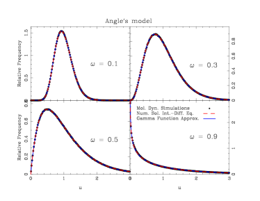
Figure 3: Angle-like’s economic model Angle (1983) which gives approximately a Gamma function as the steady state PDF plotted for different values of $\omega$. Dots are the result of the molecular dynamics numerical simulations, blue solid line is the Gamma function which approximates the steady state PDF (Eq. 14), red dashed line is the PDF which is the solution to the integro-differential equation 35. For these calculations, we take $<u>=1$.

We will now explore a mapping given in Patriarca et al. (2010) as a modification of a model introduced by Angle Angle (1983). This mapping has a parameter $\omega$ which graduates the amount of exchange of money between interacting agents. We will only explore the simplest version of all these possible Angle-like models, where one agent gives money to another one regulated by $\omega$ and a random number. It is an asymmetric model because in this model one of the agents is chosen as a winner and the other one as a loser. Other more sophisticated versions could as well be explored with this method. The precise rules to follow for this mapping are,

1. We select randomly using a uniform distribution two different agents $(i,j)$.

2. We obtain a random number between 0 and 1, $\epsilon$, generated from a uniform distribution.

3. The exchange parameter $\omega$ is maintained constant through the whole process.

4. Agent $u_{j}$ will now give some money to agent $u_{i}$ according to the following mapping,

   $$u^{\prime}_{i} = u_{i}+\epsilon\;\omega\;u_{j},$$

   $$u^{\prime}_{j} = u_{j}-\epsilon\;\omega\;u_{j},$$

   $$i,j = 1\ldots N.$$ (24)

   As before, $u_{i}$, $u_{j}$, $u^{\prime}_{i}$ and $u^{\prime}_{j}$ are the amount of money before and after the interaction of agent $i$ and $j$ respectively.

5. The application of all of the above “rules” will be denoted as “step”. These steps are successively and indefinitely repeated.

The steady state PDF in the numerical simulations of this mapping are approximated by a Gamma distribution (Eq. 14), where $\langle u\rangle$ is the mean wealth of the ensemble of agents, $a$ is given by Eq. 16 and $n$ verifies the relationship

$$n=\frac{3-2\omega}{2\omega}.$$ (25)

This function, together with a molecular dynamics simulation of the model are shown in Fig. 3. Although this Gamma function apparently fits very well the numerical simulation, we will show here that in fact it is just an approximation to the PDF and it is only exact for the cases where $\omega=1$ or $\omega=1/2$.

Let us now obtain the analytical expression for the PDF. We will proceed as before. Rule 1 will deplete the PDF for those particular values of $u$

$$\frac{\partial f(u_{i})}{\partial t}\sim-f(u_{i}),$$ (26)

and

$$\frac{\partial f(u_{j})}{\partial t}\sim-f(u_{j}).$$ (27)

From Eqs. 4 we can derive the limits of the variables. From the first of these equations (4) we obtain the inequalities

$$u_{i}<u^{\prime}_{i}<u_{i}+\omega\;u_{j},$$ (28)

from which we see that the variable $u^{\prime}_{i}$ is spanning an interval of length $\omega\;u_{j}$. This interval is where the probability from $\epsilon$ spreads over, so we need to divide by this factor. We can now split this inequation in the two following ones

$$u_{i}<u^{\prime}_{i},$$

$$u_{j}>(u^{\prime}_{i}-u_{i})/\omega,$$ (29)

and from the second equation of the mapping (4) we obtain

$$u_{j}>u^{\prime}_{j},$$

$$u_{j}<u^{\prime}_{j}/(1-\omega).$$ (30)

The increment of the PDF coming from the first equation of the mapping 4 will then be

$$\frac{\partial f(u^{\prime}_{i})}{\partial t}\sim\int_{0}^{u^{\prime}_{i}}\mathrm{d}u_{i}\int_{(u^{\prime}_{i}-u_{i})/\omega}^{\infty}\mathrm{d}u_{j}\frac{f(u_{i})f(u_{j})}{\omega u_{j}},$$ (31)

and similarly it is obtained

$$\frac{\partial f(u^{\prime}_{j})}{\partial t}\sim\int_{u^{\prime}_{j}}^{u^{\prime}_{j}/(1-\omega)}\mathrm{d}u_{j}\int_{0}^{\infty}\mathrm{d}u_{i}\frac{f(u_{i})f(u_{j})}{\omega u_{j}}.$$ (32)

where the integration limits of $u_{i}$ go from $0$ to $\infty$ because there are no constraints on this variable in the second of Eqs. 4. Since $f(u_{i})$ is normalized we can remove it from this expression,

$$\frac{\partial f(u^{\prime}_{j})}{\partial t}\sim\int_{u^{\prime}_{j}}^{u^{\prime}_{j}/(1-\omega)}\mathrm{d}u_{j}\frac{f(u_{j})}{\omega u_{j}}.$$ (33)

The final expression (Eq. 4) for the evolution of the PDF is

$$N\frac{\partial f(u)}{\partial t} =$$ (34)

$$- 2f(u)$$

$$+ \int_{0}^{u}\mathrm{d}u_{1}\int_{(u-u_{1})/\omega}^{\infty}\mathrm{d}u_{2}\frac{f(u_{1})f(u_{2})}{\omega u_{2}}$$

$$+ \int_{u}^{u/(1-\omega)}\mathrm{d}u_{2}\frac{f(u_{2})}{\omega u_{2}},$$

where we have again written the dummy variable generically as $u$, $u_{1}$ and $u_{2}$ and $N$ is the normalization factor of $\partial f(u)/\partial t$.

The steady state PDF can now be readily derived from it by setting $\partial f(u)/\partial t=0$,

$$f_{eq}(u)=$$ (35)

$$+ \frac{1}{2}\int_{0}^{u}\mathrm{d}u_{1}\int_{(u-u_{1})/\omega}^{\infty}\mathrm{d}u_{2}\frac{f_{eq}(u_{1})f_{eq}(u_{2})}{\omega u_{2}}$$

$$+ \frac{1}{2}\int_{u}^{u/(1-\omega)}\mathrm{d}u_{2}\frac{f_{eq}(u_{2})}{\omega u_{2}}.$$

We can solve this integro-differential equation iteratively by substituting $f(u)$ with the known approximate solution 14 in the right hand side of Eq. 35 to give a second order approximation in the left hand side. Usually one iteration is enough to obtain a more precise solution. The solution of this procedure is shown in Fig. 3 as a red dashed line. We can see in this figure that this solution is indistinguishable from the first approximation in Eq. 14 shown in Fig. 3 as a solid blue line, but they are not exactly the same, as we will demonstrate now.

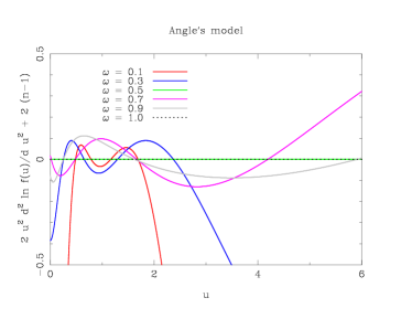
Figure 4: Plot of $2u^{2}\;\frac{\mathrm{d}^{2}\ln f(u)}{\mathrm{d}u^{2}}+2(n-1)$, where the first term has been calculated using Eq. IV, as a function of $u$. It is observed that the Gamma function is an exact solution only for $\omega$ equal $1$ or $1/2$. For these calculations, we take $<u>=1$.

If the Gamma function (Eq. 14) is indeed an exact solution of Eq. 35, the second derivative of the logarithm of both expressions should also match. The second derivative of the logarithm of the Gamma function (Eq. 14) is

$$\frac{\mathrm{d}^{2}\ln f_{eq}(u)}{\mathrm{d}u^{2}}=-\frac{(n-1)}{u^{2}}.$$ (36)

If we now multiply by $2u^{2}$ we obtain a constant,

$$2\;u^{2}\;\frac{\mathrm{d}^{2}\ln f_{eq}(u)}{\mathrm{d}u^{2}}=-2(n-1).$$ (37)

Repeating this same calculation in Eq. 35 by introducing the Gamma function (Eq. 14) in its right hand side, and doing some more elaborate calculations, we find the result,

$$2u^{2}\;\frac{\mathrm{d}^{2}\ln f_{eq}(u)}{\mathrm{d}u^{2}}=$$

$$-\int_{0}^{u}\mathrm{d}u_{1}(n-1)\frac{a(u-u_{1})^{(n-2)}u_{1}^{(n-1)}}{\omega^{n}u^{(n-2)}}\mathrm{e}^{\frac{n}{<u>}\frac{\omega-1}{\omega}u_{1}}$$

$$-\frac{\mathrm{e}^{-\frac{n}{<u>}\frac{\omega\;u}{1-\omega}}}{\omega(1-\omega)^{(n-1)}}\left(1+\frac{n}{<u>}\frac{\omega\;u}{1-\omega}\right)$$

$$+\frac{1}{\omega}.$$ (38)

The integral can be solved analytically to finally give,

$$2u^{2}\;\frac{\mathrm{d}^{2}\ln f_{eq}(u)}{\mathrm{d}u^{2}}=$$

$$-\frac{a(n-1)u^{n}\Gamma(n-1)\Gamma(n)}{\omega^{n}\Gamma(2n-1)}~{}_{1}F_{1}\left(n,2n-1,\frac{n}{<u>}\frac{\omega-1}{\omega}u\right)$$

$$-\frac{\mathrm{e}^{-\frac{n}{<u>}\frac{\omega\;u}{1-\omega}}}{\omega(1-\omega)^{(n-1)}}\left(1+\frac{n}{<u>}\frac{\omega\;u}{1-\omega}\right)$$

$$+\frac{1}{\omega},$$ (39)

where $~{}_{1}F_{1}$ is the confluent hypergeometric function. If $f(u)$ is really a Gamma function, the subtraction of Eq. IV from the expected result in Eq. 37 should give zero. So the question to be answered in this case is:

$$2u^{2}\;\frac{\mathrm{d}^{2}\ln f_{eq}(u)}{\mathrm{d}u^{2}}+2(n-1)=0\;?$$ (40)

If this result is not zero, it indicates that $f_{eq}(u)$ is not exactly a Gamma function. Results of these calculations are shown in Fig. 4 for different values of $\omega$. As it can be seen, the only results that makes this difference equal to zero over the whole domain of $u$ are $\omega=1$ or $1/2$. Let us prove it.

If $\omega=1$ then $n=1/2$ (Eq. 25) and the first two terms of the right hand side of Eq. IV are zero, leaving Eq. 40 as

$$\frac{1}{\omega}+2(n-1)=0,$$ (41)

which we can readily verify is identically zero.

If $\omega=1/2$ then $n=2$ and the hypergeometric function can be simplified to

$$\frac{~{}_{1}F_{1}}{\Gamma(2n-1)}=\frac{\mathrm{e}^{-2\frac{u}{<u>}}(-1-2\frac{u}{<u>})}{4\frac{u^{2}}{<u>^{2}}}+\frac{1}{4u^{2}/<u>^{2}}.$$ (42)

The first term of the right hand side of Eq. IV is then

$$-4\mathrm{e}^{-2\frac{u}{<u>}}\left(-1-2\frac{u}{<u>}\right)-4.$$ (43)

Inserting the values of $\omega$ and $n$, we can readily verify that the second term of the right hand side of Eq. IV is

$$-4\mathrm{e}^{-2\frac{u}{<u>}}\left(1+2\frac{u}{<u>}\right).$$ (44)

Adding both together with the last term of Eq. IV and introducing this result in Eq. 40 gives

$$-4+\frac{1}{\omega}+2(n-1)=0,$$ (45)

which we can verify is true.

To calculate the relaxation times we proceed as before. We can simplify the evolution equation (Eq. 34) close to equilibrium to

$$N\frac{\partial f(u)}{\partial t}\simeq-2f(u)+2f_{eq}(u).$$ (46)

And again, the relaxation time will be $\tau=N/2$ collisions.

V Conclusion

A step by step guide to derive the dynamical evolution equations of the PDFs of economic models involving money exchange between interacting agents, or for that matter, any other type of similar mappings, has been explained. The equilibrium distribution can be found by exploring its stationary solutions. This leads to an integro-differential equation which can be solved analytically in some cases and numerically in others.

Dragulescu and Yakovenko’s mapping Dragulescu and Yakovenko (2000) can be solved analytically giving exactly an exponential distribution (see Fig. 1). Chakraborti and Chakrabarti’s model Chakraborti and Chakrabarti (2000) can be approximated by a Gamma function, but this result is not precise, especially for low values of the savings parameter, $\lambda$. In this case the numerical solution of the integro-differential equation provides a better fit to the molecular dynamics numerical simulations (Fig. 2). Angle-like’s model Angle (1983) steady state PDF can be approximated very well by a Gamma function (Fig. 3), but according to the more exact integro-differential equations derived here, it is not an exact solution to the problem except for values of the money exchange parameter, $\omega$, of $1$ or $1/2$ (Fig. 4).

This technique should prove useful to get insights into the type of PDFs we can expect from a particular mapping, coming this mapping from an economic exchange model or from a gas with colliding particles. The exchange rules, in the case of economic models, or the collision specifications, in the case of gases, will determine which kind of PDFs the system will reach in the steady state. It is interesting to draw this parallelism, because in the economic case, and with the models shown here, we have mappings which are not symmetric in time (the equations to deplete and increment the PDFs in one time step are totally different) which give rise to distributions of the Gamma function family. In the case of gases, and in particular with the Boltzmann integro-differential equation, the collisions are symmetric in time (the equations to deplete and increment the PDFs in one time step are symmetrical), giving rise to many interesting properties, like a Gaussian function for the steady state PDF and the possibility to prove analytically Boltzmann’s H theorem.

It should be noted that we are obtaining the time evolution equations of the PDFs, and not only the stationary solutions. This should allow the study of the dynamical evolution of these systems, something which is key to economics, which as we know is not static. This has been illustrated in this paper by calculating the relaxation times of these system, but many other applications could be devised.