Nonperturbative calculations in light-front QED

Abstract:

The methods of light-front quantization and Pauli–Villars regularization are applied to a nonperturbative calculation of the dressed-electron state in quantum electrodynamics. This is intended as a test of the methods in a gauge theory, as a precursor to possible methods for the nonperturbative solution of quantum chromodynamics. The electron state is truncated to include at most two photons and no positrons in the Fock basis, and the wave functions of the dressed state are used to compute the electrons’s anomalous magnetic moment. A choice of regularization that preserves the chiral symmetry of the massless limit is critical for the success of the calculation.

1 Introduction

The purpose of this work is to explore a nonperturbative method that can be used to solve for the bound states of quantum field theories, in particular QCD. The problem is notoriously difficult, and there are only a few approaches. These include lattice gauge theory [1], the transverse lattice [2], Dyson–Schwinger equations [3], Bethe–Salpeter equation, similarity transformations combined with construction of effective fields [4], and light-front Hamiltonians with either standard [5] or sector-dependent parameterizations [6, 7, 8]. We use the light-front Hamiltonian approach with Pauli–Villars (PV) [9] regularizaton and standard parameterization, where the bare parameters of the Lagrangian do not depend on the Fock sector. As a test in a gauge theory, we consider light-front QED and specifically the eigenstate of the dressed electron and its anomalous moment [10, 11, 12, 13].

We use light-cone coordinates [14, 15], chosen in order to have well-defined Fock-state expansions and a simple vacuum. The time coordinate is $x^{+}=t+z$ and the space coordinates are $\underline{x}=(x^{-},\vec{x}_{\perp})$, with $x^{-}\equiv t-z$ and $\vec{x}_{\perp}=(x,y)$. The light-cone energy is $p^{-}=E-p_{z}$, and the three-momentum is $\underline{p}=(p^{+},\vec{p}_{\perp})$, with $p^{+}\equiv E+p_{z}$ and $\vec{p}_{\perp}=(p_{x},p_{y})$. The mass-shell condition $p^{2}=m^{2}$ becomes $p^{-}=\frac{m^{2}+p_{\perp}^{2}}{p^{+}}$. The simple vacuum follows from the positivity of the plus component of the momentum: $p^{+}\equiv\sqrt{m^{2}+p_{z}^{2}+p_{\perp}^{2}}+p_{z}>0$.

To regulate QED, we use the Pauli–Villars technique [9]. The basic idea is to subtract from each integral a contribution of the same form but of a PV particle with a much larger mass. This can be done by adding negative metric particles to the Lagrangian. A particular advantage of PV regularization is preservation of at least some symmetries; in particular, it is automatically relativistically covariant.

From the PV-regulated light-front QED Lagrangian, we construct the Hamiltonian ${\cal P}^{-}$ and solve the mass eigenvalue problem ${\cal P}^{-}|\underline{P}\rangle=\frac{M^{2}}{P^{+}}|\underline{P}\rangle$ in the approximation that the electron eigenstate is a truncated Fock-state expansion with at most two photons and no positrons. From this approximate eigenstate, we compute the anomalous magnetic moment, as a test of the method.

2 Light-front QED

The light-front QED Lagrangian with one PV fermion and two PV photons is

$${\cal L} = \sum_{i=0}^{2}(-1)^{i}\left[-\frac{1}{4}F_{i}^{\mu\nu}F_{i,\mu\nu}+\frac{1}{2}\mu_{i}^{2}A_{i}^{\mu}A_{i\mu}-\frac{1}{2}\left(\partial^{\mu}A_{i\mu}\right)^{2}\right]$$

$$+\sum_{i=0}^{1}(-1)^{i}\bar{\psi_{i}}(i\gamma^{\mu}\partial_{\mu}-m_{i})\psi_{i}-e_{0}\bar{\psi}\gamma^{\mu}\psi A_{\mu},$$

with

$$\psi=\sum_{i=0}^{1}\psi_{i},\;\;A_{\mu}=\sum_{i=0}^{2}\sqrt{\xi_{i}}A_{i\mu},\;\;F_{i\mu\nu}=\partial_{\mu}A_{i\nu}-\partial_{\nu}A_{i\mu}.$$ (2)

The coupling coefficients $\xi_{i}$ are constrained by $\xi_{0}=1$ and $\sum_{i=0}^{2}(-1)^{i}\xi_{i}=0$, and the requirement of chiral symmetry restoration in the limit of zero electron mass. At one loop, the chiral symmetry constraint becomes [10] $\sum_{i=0}^{2}(-1)^{i}\xi_{i}\frac{\mu_{i}^{2}/m_{1}^{2}}{1-\mu_{i}^{2}/m_{1}^{2}}\ln(\mu_{i}^{2}/m_{1}^{2})=0$; for nonperturbative solutions with more than one photon in the basis, the constraint must be imposed numerically [13].

The light-front Hamiltonian without antifermion terms is then of the form [12]

$${\cal P}^{-}=\sum_{i,s}\int d\underline{p}\frac{m_{i}^{2}+p_{\perp}^{2}}{p^{+}}(-1)^{i}b_{i,s}^{\dagger}(\underline{p})b_{i,s}(\underline{p})$$

$$+\sum_{l,\mu}\int d\underline{k}\frac{\mu_{l}^{2}+k_{\perp}^{2}}{k^{+}}(-1)^{l}\epsilon^{\mu}a_{l\mu}^{\dagger}(\underline{k})a_{l\mu}(\underline{k})$$

$$+\sum_{i,j,l,s,\mu}\int d\underline{p}d\underline{q}\left\{b_{i,s}^{\dagger}(\underline{p})\left[b_{j,s}(\underline{q})V^{\mu}_{ij,2s}(\underline{p},\underline{q})\right.\right.$$

$$\left.\left.\rule{36.135pt}{0.0pt}+b_{j,-s}(\underline{q})U^{\mu}_{ij,-2s}(\underline{p},\underline{q})\right]\sqrt{\xi_{l}}a_{l\mu}^{\dagger}(\underline{q}-\underline{p})+H.c.\right\},$$

with $\epsilon^{\mu}=(-1,1,1,1)$ and the vertex functions given in [12].

We work in a frame where the total transverse momentum $\vec{P}_{\perp}$ is zero and expand the eigenfunction for the dressed-fermion state with total $J_{z}=\pm\frac{1}{2}$ in a Fock basis as

$$|\psi^{\pm}(\underline{P})\rangle=\sum_{i}z_{i}b_{i\pm}^{\dagger}(\underline{P})|0\rangle+\sum_{ijs\mu}\int d\underline{k}C_{ijs}^{\mu\pm}(\underline{k})b_{is}^{\dagger}(\underline{P}-\underline{k})a_{j\mu}^{\dagger}(\underline{k})|0\rangle$$

$$+\sum_{ijks\mu\nu}\int d\underline{k_{1}}d\underline{k_{2}}C_{ijks}^{\mu\nu\pm}(\underline{k_{1}},\underline{k_{2}})\frac{1}{\sqrt{1+\delta_{jk}\delta_{\mu\nu}}}b_{is}^{\dagger}(\underline{P}-\underline{k_{1}}-\underline{k_{2}})a_{j\mu}^{\dagger}(\underline{k_{1}})a_{k\nu}^{\dagger}(\underline{k_{2}})|0\rangle,$$

where we have truncated the expansion to include at most two photons. The $z_{i}$ are the amplitudes for the bare electron states, with $i=0$ for the physical electron and $i=1$ for the PV electron. The $C_{ijs}^{\mu\pm}$ are the two-body wave functions for Fock states with an electron of flavor $i$ and spin component $s$ and a photon of flavor $j=0$, 1 or 2 and field component $\mu$, expressed as functions of the photon momentum. The upper index of $\pm$ refers to the $J_{z}$ value of $\pm\frac{1}{2}$ for the eigenstate. Similarly, the $C_{ijks}^{\mu\nu\pm}$ are the three-body wave functions for the states with one electron and two photons, with flavors $j$ and $k$ and field components $\mu$ and $\nu$.

The Fock expansion is an eigenstate of the light-front Hamiltonian ${\cal P}^{-}$ with eigenvalue
$M^{2}/P^{+}$. The wave functions then satisfy the following coupled integral equations:

$$[M^{2}-m_{i}^{2}]z_{i} = \int d\underline{q}\sum_{j,l,\mu}\sqrt{\xi_{l}}(-1)^{j+l}\epsilon^{\mu}P^{+}\left[V_{ji\pm}^{\mu*}(\underline{P}-\underline{q},\underline{P})C_{jl\pm}^{\mu\pm}(\underline{q})\right.$$

$$\rule{72.26999pt}{0.0pt}\left.+U_{ji\pm}^{\mu*}(\underline{P}-\underline{q},\underline{P})C_{jl\mp}^{\mu\pm}(\underline{q})\right],$$

$$\left[M^{2}-\frac{m_{i}^{2}+q_{\perp}^{2}}{(1-y)}-\frac{\mu_{l}^{2}+q_{\perp}^{2}}{y}\right]C_{ils}^{\mu\pm}(\underline{q})$$

$$= \sqrt{\xi_{l}}\sum_{j}(-1)^{j}z_{j}P^{+}\left[\delta_{s,\pm 1/2}V_{ijs}^{\mu}(\underline{P}-\underline{q},\underline{P})+\delta_{s,\mp 1/2}U_{ij,-s}^{\mu}(\underline{P}-\underline{q},\underline{P})\right]$$

$$+\sum_{ab\nu}(-1)^{a+b}\epsilon^{\nu}\int d\underline{q}^{\prime}\frac{2\sqrt{\xi_{b}}}{\sqrt{1+\delta_{bl}\delta^{\mu\nu}}}\left[V_{ais}^{\nu*}(\underline{P}-\underline{q}^{\prime}-\underline{q},\underline{P}-\underline{q}^{\prime})C_{abls}^{\nu\mu\pm}(\underline{q}^{\prime},\underline{q})\right.$$

$$\rule{144.54pt}{0.0pt}\left.+U_{ais}^{\nu*}(\underline{P}-\underline{q}^{\prime}-\underline{q},\underline{P}-\underline{q}^{\prime})C_{abl,-s}^{\nu\mu\pm}(\underline{q}^{\prime},\underline{q})\right],$$

$$\left[M^{2}-\frac{m_{i}^{2}+(\vec{q}_{1\perp}+\vec{q}_{2\perp})^{2}}{(1-y_{1}-y_{2})}-\frac{\mu_{j}^{2}+q_{1\perp}^{2}}{y_{1}}-\frac{\mu_{l}^{2}+q_{2\perp}^{2}}{y_{2}}\right]C_{ijls}^{\mu\nu\pm}(\underline{q}_{1},\underline{q}_{2})$$

$$= \frac{\sqrt{1+\delta_{jl}\delta^{\mu\nu}}}{2}\sum_{a}(-1)^{a}\left\{\sqrt{\xi_{j}}\left[V_{ias}^{\mu}(\underline{P}-\underline{q}_{1}-\underline{q}_{2},\underline{P}-\underline{q}_{2})C_{als}^{\nu\pm}(\underline{q}_{2})\right.\right.$$

$$\rule{144.54pt}{0.0pt}\left.+U_{ia,-s}^{\mu}(\underline{P}-\underline{q}_{1}-\underline{q}_{2},\underline{P}-\underline{q}_{2})C_{al,-s}^{\nu\pm}(\underline{q}_{2})\right]$$

$$\rule{72.26999pt}{0.0pt}+\sqrt{\xi_{l}}\left[V_{ias}^{\nu}(\underline{P}-\underline{q}_{1}-\underline{q}_{2},\underline{P}-\underline{q}_{1})C_{ajs}^{\mu\pm}(\underline{q}_{1})\right.$$

$$\left.\left.\rule{144.54pt}{0.0pt}+U_{ia,-s}^{\nu}(\underline{P}-\underline{q}_{1}-\underline{q}_{2},\underline{P}-\underline{q}_{1})C_{aj,-s}^{\mu\pm}(\underline{q}_{1})\right]\right\}.$$

The anomalous moment $a_{e}$ can be computed from the spin-flip matrix element of the electromagnetic current $J^{+}$ [16]. At zero momentum transfer, we have $a_{e}=F_{2}(0)$ and

$$a_{e} = m_{e}\sum_{s\mu}\int d\underline{k}\epsilon^{\mu}\sum_{j=0,2}\xi_{j}\left(\sum_{i^{\prime}=0}^{1}\sum_{k^{\prime}=j/2}^{j/2+1}\frac{(-1)^{i^{\prime}+k^{\prime}}}{\sqrt{\xi_{k^{\prime}}}}C_{i^{\prime}k^{\prime}s}^{\mu+}(\underline{k})\right)^{*}$$

$$\times y\left(\frac{\partial}{\partial k_{x}}+i\frac{\partial}{\partial k_{y}}\right)\left(\sum_{i=0}^{1}\sum_{k=j/2}^{j/2+1}\frac{(-1)^{i+k}}{\sqrt{\xi_{k}}}C_{iks}^{\mu-}(\underline{k})\right)$$

$$+m_{e}\sum_{s\mu\nu}\int d\underline{k_{1}}d\underline{k_{2}}\sum_{j,k=0,2}\xi_{j}\xi_{k}$$

$$\rule{72.26999pt}{0.0pt}\times\left(\sum_{i^{\prime}=0}^{1}\sum_{l^{\prime}=j/2}^{j/2+1}\sum_{m^{\prime}=k/2}^{k/2+1}\frac{(-1)^{i^{\prime}+l^{\prime}+m^{\prime}}}{\sqrt{\xi_{l^{\prime}}\xi_{m^{\prime}}}}\frac{\sqrt{2}C_{i^{\prime}l^{\prime}m^{\prime}s}^{\mu\nu+}(\underline{k_{1}},\underline{k_{2}})}{\sqrt{1+\delta_{l^{\prime}m^{\prime}}\delta_{\mu\nu}}}\right)^{*}$$

$$\times\sum_{a}\left[y_{a}\left(\frac{\partial}{\partial k_{ax}}+i\frac{\partial}{\partial k_{ay}}\right)\right]\left(\sum_{i=0}^{1}\sum_{l=j/2}^{j/2+1}\sum_{m=k/2}^{k/2+1}\frac{(-1)^{i+l+m}}{\sqrt{\xi_{l}\xi_{m}}}\frac{\sqrt{2}C_{ilms}^{\mu\nu-}(\underline{k_{1}},\underline{k_{2}})}{\sqrt{1+\delta_{lm}\delta_{\mu\nu}}}\right).$$

The terms that depend on the three-body wave functions $C_{ilms}^{\mu\nu\pm}$ are higher order in $\alpha$ than the leading two-body terms. Given the numerical errors in the leading terms, these three-body contributions are not significant and are not evaluated. The important three-body contributions come from the couplings of the three-body wave functions that will enter the calculation of the two-body wave functions.

3 Solution of the Coupled Equations

The first and third equations of the coupled system, (2) and (2), can be solved for the bare-electron amplitudes and one-electron/two-photon wave functions, respectively, in terms of the one-electron/one-photon wave functions. Substitution of these solutions into the second integral equation (2) yields a reduced integral eigenvalue problem in the one-electron/one-photon sector:

$$\left[M^{2}-\frac{m_{i}^{2}+q_{\perp}^{2}}{1-y}-\frac{\mu_{j}^{2}+q_{\perp}^{2}}{y}\right]C_{ijs}^{\mu\pm}(y,q_{\perp})=\frac{\alpha}{2\pi}\sum_{i^{\prime}}\frac{I_{iji^{\prime}}(y,q_{\perp})}{1-y}C_{i^{\prime}js}^{\mu\pm}(y,q_{\perp})$$

$$\rule{72.26999pt}{0.0pt}+\frac{\alpha}{2\pi}\sum_{i^{\prime}j^{\prime}s^{\prime}\nu}\epsilon^{\nu}\int_{0}^{1}dy^{\prime}dq_{\perp}^{\prime 2}J_{ijs,i^{\prime}j^{\prime}s^{\prime}}^{(0)\mu\nu}(y,q_{\perp};y^{\prime},q^{\prime}_{\perp})C_{i^{\prime}j^{\prime}s^{\prime}}^{\nu\pm}(y^{\prime},q^{\prime}_{\perp})$$

$$\rule{72.26999pt}{0.0pt}+\frac{\alpha}{2\pi}\sum_{i^{\prime}j^{\prime}s^{\prime}\nu}\epsilon^{\nu}\int_{0}^{1-y}dy^{\prime}dq_{\perp}^{\prime 2}J_{ijs,i^{\prime}j^{\prime}s^{\prime}}^{(2)\mu\nu}(y,q_{\perp};y^{\prime},q^{\prime}_{\perp})C_{i^{\prime}j^{\prime}s^{\prime}}^{\nu\pm}(y^{\prime},q^{\prime}_{\perp}).$$

There is a total of 48 coupled equations, with $i=0,1$; $j=0,1,2$; $s=\pm\frac{1}{2}$; and $\mu=\pm,(\pm)$.

The first term on the right-hand side of (3) is the self-energy contribution [12]:

$$I_{ili^{\prime}}(y,q_{\perp})=\sum_{a,b}(-1)^{i^{\prime}+a+b}\xi_{b}\int_{0}^{1}\frac{dx}{x}\frac{d^{2}k_{\perp}}{\pi}\frac{m_{i}m_{i^{\prime}}-2\frac{m_{i}+m_{i^{\prime}}}{1-x}m_{a}+\frac{m_{a}^{2}+k_{\perp}^{2}}{(1-x)^{2}}}{\Lambda_{l}-\frac{m_{a}^{2}+k_{\perp}^{2}}{1-x}-\frac{\mu_{b}^{2}+k_{\perp}^{2}}{x}},$$ (10)

with

$$\Lambda_{l}\equiv\mu_{l}^{2}+(1-y)M^{2}-\frac{\mu_{l}^{2}+q_{\perp}^{2}}{y}.$$ (11)

The kernels $J^{(0)}$ and $J^{(2)}$ in the second and third terms correspond to interactions with zero or two photons in intermediate states. Details of these kernels can be found in [13] and [11].

The presence of the flavor changing self-energies, the $I_{ili^{\prime}}$ with $i\neq i^{\prime}$, generates a fermion flavor mixing of the two-body wave functions [12]. To resolve this, we write the integral equations for these wave functions in the form

$$A_{0j}C_{0js}^{\mu\pm}-B_{j}C_{1js}^{\mu\pm}=-\frac{\alpha}{2\pi}J_{0js}^{\mu\pm},\;\;B_{j}C_{0js}^{\mu\pm}+A_{1j}C_{1js}^{\mu\pm}=-\frac{\alpha}{2\pi}J_{1js}^{\mu\pm},$$ (12)

where $A_{ij}$ and $B_{j}$ are defined by

$$A_{ij}=\frac{m_{i}^{2}+q_{\perp}^{2}}{1-y}+\frac{\mu_{j}^{2}+q_{\perp}^{2}}{y}+\frac{\alpha}{2\pi}\frac{I_{iji}}{1-y}-M^{2},\;\;B_{j}=\frac{\alpha}{2\pi}\frac{I_{1j0}}{1-y}=-\frac{\alpha}{2\pi}\frac{I_{0j1}}{1-y},$$ (13)

and $J_{ijs}^{\mu\pm}$ is given by

$$J_{ijs}^{\mu\pm} = \sum_{i^{\prime}j^{\prime}s^{\prime}\nu}\epsilon^{\nu}\int_{0}^{1}dy^{\prime}dq_{\perp}^{\prime 2}J_{ijs,i^{\prime}j^{\prime}s^{\prime}}^{(0)\mu\nu}(y,q_{\perp};y^{\prime},q^{\prime}_{\perp})C_{i^{\prime}j^{\prime}s^{\prime}}^{\nu\pm}(y^{\prime},q^{\prime}_{\perp})$$

$$+\sum_{i^{\prime}j^{\prime}s^{\prime}\nu}\epsilon^{\nu}\int_{0}^{1-y}dy^{\prime}dq_{\perp}^{\prime 2}J_{ijs,i^{\prime}j^{\prime}s^{\prime}}^{(2)\mu\nu}(y,q_{\perp};y^{\prime},q^{\prime}_{\perp})C_{i^{\prime}j^{\prime}s^{\prime}}^{\nu\pm}(y^{\prime},q^{\prime}_{\perp}).$$

We then construct wave functions that mix fermion flavors and diagonalize the left-hand side of (12): $\tilde{f}_{ijs}^{\mu\pm}=A_{ij}C_{ijs}^{\mu\pm}+(-1)^{i}B_{j}C_{1-i,js}^{\mu\pm}$. Solution of the resulting integral equations for the $f_{ijs}^{\mu\pm}$ [13] yields $\alpha$ as a function of $m_{0}$ and the PV masses. Then for given values of PV masses, we can seek the value of $m_{0}$ for which $\alpha$ takes the standard physical value $e^{2}/4\pi$. The eigenproblem solution also yields the functions $\tilde{f}_{ijs}^{\mu\pm}$ which determine the wave functions $C_{ijs}^{\mu\pm}$. From these wave functions we can compute physical quantities as expectation values with respect to the projection [13] of the eigenstate onto the physical subspace.

The eigenvalue problem must first be solved for $M=0$, with the coupling strength parameter $\xi_{2}$ adjusted to yield $m_{0}=0$. This determines the value of $\xi_{2}$ that restores the chiral limit nonperturbatively. The eigenvalue problem can then be solved for $M=m_{e}$, the physical mass of the electron, and the anomalous moment calculated.

If we retain only the self-energy contributions from the two-photon intermediate states, the equations for the two-body wave functions become much simpler, and the coupled integral equations can be reduced to the one-electron sector. There, they can be solved analytically, except for the calculation of certain integrals [12].

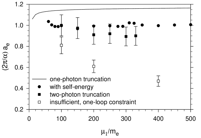
Figure 1: The anomalous moment of the electron in units of the Schwinger term ($\alpha/2\pi$) plotted versus the PV photon mass, $\mu_{1}$, with the second PV photon mass, $\mu_{2}$, set to $\sqrt{2}\mu_{1}$ and the PV electron mass $m_{1}$ equal to $2\cdot 10^{4}\,m_{e}$. The solid squares are the result of the full two-photon truncation with the correct, nonperturbative chiral constraint [13]. The open squares come from use of a perturbative, one-loop constraint. Results for the one-photon truncation [10] (solid line) and the one-photon truncation with the two-photon self-energy contribution [12] (filled circles) are included for comparison. The resolutions used for the two-photon results are $K=50$ to 150, combined with extrapolation to $K=\infty$, and $N_{\perp}=20$.

4 Results

From the solutions to the eigenvalue problems, we compute the anomalous moment at fixed PV masses and fixed numerical resolution. We then study the behavior first as a function of the numerical resolution, which requires extrapolation, and then as a function of PV masses. The numerical resolution is marked by two parameters, $K$ and $N_{\perp}$, which control the number of quadrature points used in the longitudinal and transverse directions. The numerical convergence and extrapolation are illustrated in [13].

The results of the extrapolations are plotted in Fig. 1. Each value is close to the standard Schwinger result of $\alpha/2\pi$ and independent of $\mu_{1}$, to within numerical error. The results with only the two-photon self-energy contribution are actually better than the full two-photon results. This discrepancy should be due to the absence of electron-positron contributions, which are of the same order in $\alpha$ as the two-photon contributions; without the electron-positron contributions, we lack the cancellations that typically take place between contributions of the same order.

We also see that the inclusion of the self-energy contribution is a significant improvement over the one-photon truncation. Thus, we expect that inclusion of three-photon self-energy effects will improve the two-photon results.

Figure 1 also includes results obtained for the two-photon truncation when only the one-loop chiral constraint is satisfied. Without the full nonperturbative constraint, the results are very sensitive to the PV photon mass $\mu_{1}$. This behavior repeats the pattern observed in [10] for a one-photon truncation without the corresponding one-loop constraint. The resulting $\mu_{1}$ dependence is illustrated in Fig. 2 of [10]. Thus, a successful calculation requires that the symmetry of the chiral limit be maintained.

References

• [1] For reviews of lattice theory, see M. Creutz, L. Jacobs and C. Rebbi, Phys. Rep. 95 (1983) 201; J.B. Kogut, Rev. Mod. Phys. 55 (1983) 775; I. Montvay, ibid59 (1987) 263; A.S. Kronfeld and P.B. Mackenzie, Ann. Rev. Nucl. Part. Sci. 43 (1993) 793; J.W. Negele, Nucl. Phys. A553 (1993) 47c; K.G. Wilson, Nucl. Phys. B (Proc. Suppl.) 140 (2005) 3; J.M. Zanotti, \posPoS(LAT2008)007. For recent discussions of meson properties and charm physics, see for example C. McNeile and C. Michael [UKQCD Collaboration], Phys. Rev. D 74 (2006) 014508; I. Allison et al. [HPQCD Collaboration], Phys. Rev.  D 78 (2008) 054513.
• [2] M. Burkardt and S. Dalley, Prog. Part. Nucl. Phys. 48 (2002) 317 and references therein; S. Dalley and B. van de Sande, Phys. Rev. D 67 (2003) 114507; D. Chakrabarti, A.K. De, and A. Harindranath, Phys. Rev. D 67 (2003) 076004; M. Harada and S. Pinsky, Phys. Lett. B 567 (2003) 277; S. Dalley and B. van de Sande, Phys. Rev. Lett.  95 (2005) 162001; J. Bratt, S. Dalley, B. van de Sande, and E. M. Watson, Phys. Rev. D 70 (2004) 114502. For work on a complete light-cone lattice, see C. Destri and H.J. de Vega, Nucl. Phys. B290 (1987) 363; D. Mustaki, Phys. Rev. D 38 (1988) 1260.
• [3] C.D. Roberts and A.G. Williams, Prog. Part. Nucl. Phys. 33 (1994) 477; P. Maris and C.D. Roberts, Int. J. Mod. Phys. E12 (2003) 297; P.C. Tandy, Nucl. Phys. B (Proc. Suppl.) 141 (2005) 9.
• [4] S. D. Glazek and R. J. Perry, Phys. Rev. D 78 (2008) 045011; S.D. Głazek and J. Mlynik, Phys. Rev. D 74 (2006) 105015; S.D. Głazek, Phys. Rev. D 69 (2004) 065002; S.D. Głazek and J. Mlynik, Phys. Rev. D 67 (2003) 045001; S.D. Głazek and M. Wieckowski, Phys. Rev. D 66 (2002) 016001.
• [5] S.J. Brodsky, J.R. Hiller, and G. McCartor, Phys. Rev. D 58 (1998) 025005; 60 (1999) 054506; 64 (2001) 114023; Ann. Phys. 296 (2002) 406; 305 (2003) 266; 321 (2006) 1240; S.J. Brodsky, V.A. Franke, J.R. Hiller, G. McCartor, S.A. Paston, and E.V. Prokhvatilov, Nucl. Phys. B 703 (2004) 333.
• [6] R.J. Perry, A. Harindranath, and K.G. Wilson, Phys. Rev. Lett. 65 (1990) 2959; R.J. Perry and A. Harindranath, Phys. Rev. D 43 (1991) 4051.
• [7] V. A. Karmanov, J. F. Mathiot, and A. V. Smirnov, Phys. Rev. D 77 (2008) 085028; arXiv:1006.5640 [hep-th].
• [8] J.P. Vary et al., Phys. Rev. C 81 (2010) 035205.
• [9] W. Pauli and F. Villars, Rev. Mod. Phys. 21 (1949) 434.
• [10] S.S. Chabysheva and J.R. Hiller, Phys. Rev. D 79 (2009) 114017.
• [11] S.S. Chabysheva, A nonperturbative calculation of the electron’s anomalous magnetic moment, Ph.D. thesis, Southern Methodist University ProQuest Dissertations & Theses 3369009 2009.
• [12] S.S. Chabysheva and J.R. Hiller, Ann. Phys. 325 (2010) 2435.
• [13] S.S. Chabysheva and J.R. Hiller, Phys. Rev. D 81 (2010) 074030.
• [14] P.A.M. Dirac, Rev. Mod. Phys. 21 (1949) 392.
• [15] For reviews of light-cone quantization, see M. Burkardt, Adv. Nucl. Phys. 23, 1 (2002); S.J. Brodsky, H.-C. Pauli, and S.S. Pinsky, Phys. Rep. 301 (1998) 299.
• [16] S.J. Brodsky and S.D. Drell, Phys. Rev. D 22 (1980) 2236.