Comparative Performance of Tabu Search and Simulated Annealing Heuristics for the Quadratic Assignment Problem

Abstract

For almost two decades the question of whether tabu search (TS) or simulated annealing (SA) performs better for the quadratic assignment problem has been unresolved. To answer this question satisfactorily, we compare performance at various values of targeted solution quality, running each heuristic at its optimal number of iterations for each target. We find that for a number of varied problem instances, SA performs better for higher quality targets while TS performs better for lower quality targets.

1 Introduction

The quadratic assignment problem (QAP) is a combinatorial optimization problem first introduced by Koopmans and Beckman [12]. It is NP-hard and is considered to be one of the most difficult problems to be solved optimally. The problem is defined in the following context: A set of $N$ facilities are to be located at $N$ locations. The distance between locations $i$ and $j$ is $D_{i,j}$ and the quantity of materials which flow between facilities $i$ and $j$ is $F_{i,j}$. The problem is to assign to each location a single facility so as to minimize the cost

$$C=\sum_{i=1}^{N}\sum_{j=1}^{N}F_{i,j}D_{p(i),p(j)}.$$

where $p(i)$ represents the location to which facility $i$ is assigned.

There is an extensive literature which addresses the QAP and is reviewed in [19, 7, 2, 11, 13]. With the exception of specially constructed cases, optimal algorithms have solved only relatively small instances ($N\leq 36$). Various heuristic approaches have been developed and applied to problems typically of size $N\approx 100$ or less. Two of the most successful heuristics to date for the QAP are tabu search (TS) and simulated annealing (SA). They are basic heuristics which are used alone or as components in hybrid and iterative metaheuristics.

Comparisons of the performance of SA and TS for the QAP have been inconclusive. In this work, we are able to successfully characterize the relative performance of these heuristics by performing the comparisons for various values of solution quality and by setting the number of iterations for each heuristic to the optimal one for the target solution quality.

As is common practice, we define the quality, $Q$ of a solution

$$Q\equiv\frac{C-C_{best}}{C_{best}},$$

where $C$ is the value of the objective function for the solution and $C_{best}$ is the best known value of the objective function for the instance. The lower the value of $Q$, the higher the quality.

We find that for each problem instance, there is a value of $Q$, $Q^{*}$, above which (lower quality) tabu search performs better — requires less time — than simulated annealing and below which (higher quality) simulated annealing performs better.

2 Background

The tabu search heuristic for the quadratic assignment problem consists of repeatedly swapping locations of two nodes. A single iteration of the heuristic consists of making the swap which most decreases the total cost. Under certain conditions, if a move which lowers the cost is not available, a move which raises the cost is made. To ensure that cycles of the same moves are avoided, the same move is forbidden (taboo) until a specified later iteration; we call this later iteration the eligible iteration for a given move. This eligible iteration is traditionally stored in a tabu list or tabu table. The process is repeated for a specified number of iterations.

The simulating annealing heuristic also consists of swapping locations of two facilities. In the simulated annealing approach used here [8], each possible swap is considered in turn and $\delta$, the change in cost for the potential swap, is calculated. The swap is made if $\delta$ is negative or if

$$e^{-\delta/T}>r,$$

where $T$ is an analog of temperature in physical systems that is slowly decreased according to a specified cooling schedule after each iteration and $r$ is a uniformly distributed random variable between 0 and 1. Randomly making moves which increase the cost is done to help escape from local minima.

Pardalos [19] compared the performance of four algorithms including simulated annealing and tabu search and found that “all of these approaches have almost the same performance”. Paulli [21] compared simulated annealing and tabu search and found that “when CPU time is taken into consideration, simulated annealing is clearly preferable to tabu search”. On the other hand, [5] finds that “RTS (Reactive Tabu Search) needs less CPU time than SA to reach average results in the $1\%$ [of the best known value] region”. In 1998, summarizing the situation, Cela [7] commented that “There is no general agreement concerning the comparison of the performance of simulated annealing approaches with that of tabu search approaches for the QAP”. We are not aware of any later work which has clarified the issue.

3 Approach

We address the question of whether tabu search or simulated annealing performs better for the quadratic assignment problem by recognizing that the answer depends on desired solution quality and by:

• defining a performance metric that ensures a fair comparison of different heuristics,

• determining the optimal number of iterations for a given target quality for TS and SA for each problem instance; for a fair comparison of heuristics, it is critical to run each heuristic at its optimal number of iterations for a given target solution quality.

• measuring the performance of TS and SA at multiple target qualities.

4 Performance Metric

To fairly compare heuristics, solution quality and time must be taken into account. Simulated annealing and tabu search are multi-start heuristics; many runs of the heuristic are executed, each with a different random starting configuration. A commonly used performance metric for multi-start heuristics is the percentage of these runs which attain a specified value of the quality $Q$ (typically $0.01$). However, this metric doesn’t take run time into account. Sometimes, the runs times for individual runs of the heuristics are constrained to be equal but this is problematic because, as we show below, for a fair comparison each heuristic should be run at the optimal number of iterations for the quality goal $Q$. One method of characterizing the performance of multistart heuristics with different run times employs run-time distributions of the times needed across multiple runs to achieve a certain quality goal (see e.g. [23, 1]). Instead of using distributions, we define the performance metric $\bar{T}(Q,I)$ as the average time to attain a quality goal of $Q$ during a set of runs, each run with $I$ iterations:

$$\bar{T}(Q,I)=\frac{\sum_{i}t_{i}}{N(Q,I)},$$

where $t_{i}$ is the CPU time for run $i$ and $N(Q,I)$ is the number of runs which attain a quality goal of $Q$ or better.

Because one heuristic may perform better depending on the quality goal, we calculate this performance metric not just for a single quality goal (e.g. $0.01$) but for a range of quality goals.

5 Numerical Results

We use C++ implementations of SA and TS in the public domain to perform our computational experiments. Both implementations are by Taillard, and are available at http://mistic.heig-vd .ch/taillard/. The TS code implements the robust tabu search of [24]; the SA code implements the simulated annealing heuristic of [8]. Both implementations are straightforward and a few pages each in length. We run the TS heuristic with parameter settings as described in [24]): tabu list size between $0.9N$ and $1.1N$ and aspiration function parameter equal to $2N^{2}$; there are no settable parameters for the SA implementation.

5.1 Determination of Optimal Number of Iterations

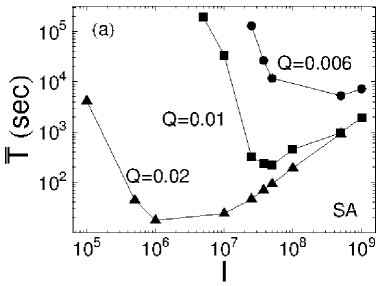
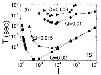
Given a fixed time in which a heuristic can be executed, there is a tradeoff between the number of iterations per run and the number of runs which can be performed. The optimal number of iterations per run to reach a quality goal of $Q$, $I_{opt}(Q)$, is the value of $I$ which minimizes $\bar{T}(Q,I)$. We determine $I_{opt}(Q))$ as follows: For various values of $I$, $I_{i}$, we run each heuristic multiple times and calculate $\bar{T}(Q,I_{i})$. Then,

$$I_{opt}(Q)=\{I_{i}|\bar{T}(Q,I_{i})=\bar{T}(Q)\}$$

where

$$\bar{T}(Q)\equiv\operatorname*{min}_{i}\bar{T}(Q,I_{i}).$$

Thus $\bar{T}(Q)$ is the value of the performance metric when the heuristic is run at $I_{opt}(Q)$ iterations.

In Fig. 1(a), using the Tai100a problem instance from QAPLIB [6] as an example, we illustrate the process of finding the optimal number of simulated annealing iterations for $Q=0.02,0.01,$ and $0.006$. The optimal number of iterations, $I_{opt}$, for each value of $Q$ is the well defined minimum value of $\bar{T}$ for each plot. For a given value of $Q$, we note the large variation in $\bar{T}$. We also note the large variation in $I_{opt}$ for the different values of $Q$. Thus, choosing a non-optimal value of iterations (e.g. a single value for the number of iterations for different $Q$) will result in an unfair characterization of the performance of the heuristic. Similarly, Fig. 1(b), illustrates the process of finding the optimal number of tabu iterations for the instance Tai100a for $Q=0.02,0.015,0.01$ and $0.009$.

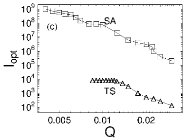
In Fig. 1(c), we plot $I_{opt}$, versus Q for SA and TS. For TS, $I_{opt}$ increases as $Q$ decreases but does not increase below $Q\approx 0.01$. We infer that for TS there is no benefit to increasing the number of iterations below this point; any improvements in quality are gained by running more random starting configurations. On the other hand, SA benefits by increasing the number of iterations as $Q$ is decreased over the complete range of $Q$ studied. The subject of an optimal number of iterations for the quality goal $Q=0$ for simulated annealing is treated analytically in [4].

5.2 Performance Comparison of SA and TS

We perform computational experiments on the following problem instances from QAPLIB [6] representing a range of problem difficulty, type and size.

• Tai100a [24] is a totally unstructured instance consisting of random distance and flow matrices.

• nug30 [17], sko100a [22], and tho150 [25] are instances in which the distances are the Manhattan distances between locations on a grid.

• lipa90a [14] is a generated problem instance with a known optimal solution.

• dre110 [9] is a structured instance consisting of a ”grid” flow matrix with non-zero entries for nearest neighbors only. It is part of a series of instances that are specifically designed to be difficult for heuristics.

For each problem instance we execute a series of runs for various values of $I$ including: $I$ = $10^{6}$, $5\cdot 10^{6}$, $10\cdot 10^{6}$, $50\cdot 10^{6}$, $100\cdot 10^{6}$, $500\cdot 10^{6}$, and $10^{9}$ for SA and $I$ = $10^{3}$, $5\cdot 10^{3}$, $10\cdot 10^{3}$, $50\cdot 10^{3}$, $100\cdot 10^{3}$, $500\cdot 10^{3}$, and $10^{6}$ for TS. For some instances, additional values of $I$ are used. As described above, for each problem instance we determine the value of $\bar{T}(Q)$ for various values of $Q$.

By plotting $\bar{T}(Q)$ for each heuristic we can compare the performance of the heuristics when they are run with the optimal number of iterations. Fig. 2 plots $\bar{T}(Q)$ versus $Q$ for the instances studied. Despite differences in details, they all share the characteristic that for each problem instance, there is a value of $Q$, $Q^{*}$, above which (lower quality) tabu search performs better — requires less time — than simulated annealing and below which (higher quality) simulated annealing performs better. SA achieves lowest known costs for all but the Tai100a instance. TS achieves the lowest known cost for three of the six instances.

In Table 1 we list the values of $Q^{*}$ for each of the instances studied. Note that if only the value $Q=0.01$ were considered, the conclusion would be simply that SA is better for some instances and TS for others. This explains why earlier studies of relative performance where not able to draw clear conclusions.

5.3 Hardness of Problem Instances

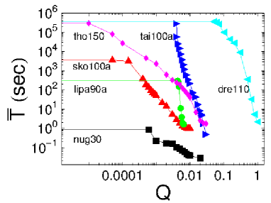
To compare the relative hardness of the problem instances studied, in Fig. 3 we plot $\bar{T}$ versus $Q$ for the problem instances in a single panel. The relative hardness of the instances for a given solution quality is given by the relative value of $\bar{T}$ at that quality. Comparing this figure with Table 1 note that $Q^{*}$ appears to be correlated with the hardness of the problem. With the exception of Tai100a, the harder the problem, the higher the value of $Q^{*}$ and thus the wider the range of $Q$ in which SA performs better than TS.

6 Discussion

How do we explain our results that, for each problem instance studied, there is a value of the quality $Q$, $Q^{*}$, above which TS performs better than SA and below which SA performs better? A possible qualitative explanation is that TS essentially uses a steepest descent method to quickly find an initial local minimum while SA finds the local minima in a more random way — sometimes making moves which increase the total cost even when moves which reduce the cost could be made first. Hence for high $Q$, TS performs better. Once a local minimum is found, however, SA is better able to escape and find a lower minimum. As opposed to TS, to attain better solution quality it is always better to run fewer SA runs with a higher number of iterations.

Areas for future research might address the following questions:

• Is similar behavior observed when comparing SA and TS applied to other combinatorially complex problems?

• When optimal numbers of iterations are used for SA and TS within such hybrid heuristics as hybrid genetic search, is the performance of the hybrid heuristic improved?

• How does the performance of other heuristics (e.g. hybrid, iterated, ANT) compare when taking solution quality into account?

• How are our findings changed if variants of TS are used? Can SA be modified to also outperform TS at high values of $Q$?

References

Table 1: Value of $Q$, $Q^{*}$ below which SA performs better than TS.

Problem	$C_{best}$	$Q^{*}$
nug30	6124 [3]	0.0014
lipa90a	360630 [14]	0.0047
sko100a	152002 [10]	0.01
tai100a	21052466 [16]	0.0125
tho150	8133398 [15]	0.025
dre110	2052 [9]	0.058

Figure 1: (a)Dependence of $\bar{T}$ on number of simulated annealing iterations $I$ for quality $Q=0.02,0.01$ and $0.006$ for the QAP instance Tai100a. (b)Dependence of $\bar{T}$ on number of tabu iterations $I$ for quality $Q=0.02,.015,0.01$ and $0.009$ for the QAP instance Tai100a. (c) Optimal number of iterations, $I_{opt}$ versus $Q$ for SA(squares) and TS (triangles).

$\begin{array}[]{cc}\epsfbox{pnug30Ro.eps}&\epsfbox{plipa90aRo.eps}\\ \epsfbox{psko100aRo.eps}&\epsfbox{ptho150Ro.eps}\\ \epsfbox{ptai100aRo.eps}&\epsfbox{pdre110Ro.eps}\end{array}$

Figure 2: $\bar{T}$ versus Q for various problem instances for SA(squares) and TS (triangles). For plots which achieve the lowest known cost for an instance ($Q=0$), we extend the line connecting the plot points to the left edge of the panel.

Figure 3: $\bar{T}$ versus $Q$ for for all problem instances studied: nug30 (squares), lipa90a (disks), sko100a (up-pointing triangles), tho150 (diamonds), tai100a (right-pointing triangles, dre110 (left-pointing triangles).

References

- [1] Aiex, R.M., M.G.C. Resende, C.C. Ribeiro. 2002. Probability distribution of solution time in GRASP: An experimental investigation. J. Heuristics 8 343-373.
- [2] K. Anstreicher. Recent advances in the solution of quadratic assignment problems, Math. Program 97 (2003) 27-42.
- [3] K.M. Anstreicher, N.W. Brixius, J.-P. Goux, J. Linderoth. Solving large quadratic assignment problems on computational grids. Math. Program 91 (2002) 563-588.
- [4] R. Azencott. Sequential simulated annealing: speed of convergence and acceleration techniques, in: Simulated Annealing Parallelization Techniques, John Wiley and Sons, (1992).
- [5] R. Battiti, G. Tecchiolli. Tabu search in the long-run - A comparison on QAP tasks. Computers and Mathematics with Applications 28 (1994) 1-8.
- [6] R.E. Burkard, E. Cela, S. E. Karish, F. Rendl. 1997. QAPLIB - A Quadratic Assignment Problem Library. J. Global Optim. 10 (1997) 391-403; http://www.seas.upenn.edu/qaplib/
- [7] E. Cela E. 1998. The Quadratic Assignment Problem: Theory and Algorithms. Kluwer, Boston, MA. 1998.
- [8] D. T. Connolly, An improved annealing scheme for the QAP, European Journal of Operational Research 46 (1990) 93-100.
- [9] Z. Drezner, P.M. Hahn, È. D. Taillard, Recent Advances for the Quadratic Assignment Problem with Special Emphasis on Instances that are Difficult for Meta-Heuristic Methods, Annals of Operations Research 139 (2005) 65-94.
- [10] C. Fleurent, J.A. Ferland. Genetic hybrids for the quadratic assignment problem, In P. Pardalos and H. Wolkowicz, editors, Quadratic assignment and related problems 16, 173-187. DIMACS Series in Discrete Mathematics and Theoretical Computer Science, 1994.
- [11] T. James, C. Rego, F. Glover. 2009. Multistart Tabu Search and Diversification Strategies for the Quadratic Assignment Problem, IEEE Tran. on Systems, Man, and Cybernetics PART A: SYSTEMS AND HUMANS bf 39 (2009) 579-596.
- [12] T. Koopmans, M. Beckman. Assignment problems and the location of economic activities, Econometrica 25 (1957) 53-76.
- [13] E.M. Loiola, N.M.M. de Abreu, P.O. Boaventuro-Netto, P. Hahn, P.T. Querido. A survey for the quadratic assignment problem, European Journal of Operational Research 176, (2007) 657-690.
- [14] Y. Li and P.M. Pardalos. Generating quadratic assignment test problems with known optimal permutations, Computational Optimization and Applications, 1 (1992) 53-76.
- [15] A. Misevicius. A modified simulated annealing algorithm for the quadratic assignment problem, Informatica, 14 (2003)497-514.
- [16] A. Misevicius. 2005. A tabu search algorithm for the quadratic assignment problem, Comput. Optim. and Appl. 30 (2005) 95-111.
- [17] C.E. Nugent, T.E. Vollman, and J. Ruml. An experimental comparison of techniques for the assignment of facilities to locations. Operations Research, 16 (1968) 150-173.
- [18] P.M. Pardalos, K.A. Murthy, T.P. Harrison. A computational comparison of local search heuristics for solving local quadratic assignment problems, Informatica 4 (1993) 172-187.
- [19] P.M. Pardalos, F. Rendl, H. Wolkowicz. The quadratic assignment problem: A survey and recent developments. Pardalos, P.M., Wolkowicz, H., eds. Quadratic Assignment and Related Problems. DIMACS Series on Discrete Mathematics and Theoretical Computer Science 16, Amer. Math. Soc., Baltimore, MD. (1994) 1-42.
- [20] P.M. Pardalos, L. S. Pitsoulis , M. G. C. Resende. Algorithm 769: Fortran subroutines for approximate solution of sparse quadratic assignment problems using GRASP, ACM Transactions on Mathematical Software (TOMS) 23 (1997) 196-208.
- [21] J. Paulli. A computational comparison of simulated annealing and tabu search applied to the quadratic assignment problem, In Ren V. V. Vidal (ed.), Applied Simulated Annealing. Springer-Verlag, Lecture Notes in Economics and Mathematical Systems (1993) 85-102.
- [22] J. Skorin-Kapov. Tabu search applied to the quadratic assignment problem, ORSA Journal on Computing 2 (1990) 33-45.
- [23] T. Stützle. Local Search Algorithms for Combinatorial Problems - Analysis, Improvements, and New Applications. PhD thesis, Darmstadt University of Technology, Department of Computer Science, 1998.
- [24] È. Taillard. Robust taboo search for the quadratic assignment problem, Parallel Comput. 17 (1991) 443-455.
- [25] U.W. Thonemann, A. Bölte. An improved simulated annealing algorithm for the quadratic assignment problem. Working paper, School of Business, Department of Production and Operations Research, University of Paderborn, Germany, 1994.