Analysis of coupled transport phenomena in concrete
at elevated temperatures

Abstract

In this paper, we study a non-linear numerical scheme arising from the implicit time discretization of the Bažant-Thonguthai model for hygro-thermal behavior of concrete at high temperatures. Existence and uniqueness of the time-discrete solution in two dimensions is established using the theory of pseudomonotone operators in Banach spaces. Next, the spatial discretization is accomplished by the conforming finite element method. An illustrative numerical example shows that the model reproduces well the rapid increase of pore pressure in wet concrete due to extreme heating. Such phenomenon is of particular interest for the safety assessment of concrete structures prone to thermally-induced spalling.

1 Introduction

The hygro-thermal behavior of concrete plays a crucial role in the assessment of the reliability and lifetime of concrete structures. The heat and mass transfer processes become particularly important at high temperatures, where the increased pressure in pores may lead to catastrophic service failures. Since high-temperature experiments are very expensive, predictive modeling of humidity migration and pore pressure developments can result in significant economic savings. The first mathematical models of concrete exposed to temperatures exceeding $100^{\circ}$C were formulated by Bažant and Thonguthai in [1]. Since then, a considerable effort has been invested into detailed numerical simulations of concrete structures subject to high temperatures. However, much less attention has been given to the qualitative properties of the model, as well as of the related numerical methods.

In particular, the only related work the authors are aware of is due to Dalík et al. [3], who analyzed the numerical solution of the Kiessl model [8] for moisture and heat transfer in porous materials. They proved some existence and regularity results and suggested an efficient numerical approach to the solution of the resulting system of highly non-liner equations. However, the Kiessl model is valid for limited temperature range only and as such it is inappropriate for high-temperature applications. In this contribution, we extend the work [3] by proving the existence and uniqueness of an approximate solution for the Bažant-Thonguthai model, arising from the semi-implicit discretization in time. A fully discrete algorithm is then obtained by standard finite element discretization and its performance is illustrated for a model problem of a concrete segment exposed to transient heating according to the standard ISO fire curve. Here, the focus is on the short-term pore pressure build up, which is decisive for the assessment of so-called thermal spalling during fire.

At this point, it is fair to mention that the Bažant-Thonguthai model was later extended towards more detailed multi-phase description, see e.g. the works of Gawin et al. [6], Tenchev et al. [13] and Davie et al. [4] for specific examples. When compared to the original version, these advanced models provide better insight into physical and chemical processes in concrete (such as influence of gel water, pore water, capillary water, chemical reactions at elevated temperatures, etc.). Such potential increase in accuracy, however, comes at the expense of increased number of parameters, which typically reflect complex multi-scale nature of concrete. Hence, their experimental determination is rather complicated and the parameters can often only be calibrated by sub-scale simulations. Therefore, in this work we adopt a pragmatic approach and consider the single-phase Bažant-Thonguthai model with parameters provided by heuristic relations, obtained from regression of reliable macroscopic experiments.

The paper is organized as follows. In Section 2, we present the general single-phase, purely macroscopic, model for prediction of hygro-thermal behavior of heated concrete. In Section 3, we introduce basic notation, the appropriate function spaces and formulate the problem in the strong and variational sense. In Section 4.1, we specify our assumptions on data and modify structure conditions to obtain a reasonably simple but still realistic model of hygro-thermal behavior of concrete at high temperatures due to Bažant and Thonguthai [1]. An application of the Rothe method of discretization in time leads to a coupled system of semilinear steady-state equations, which (together with the appropriate boundary conditions) form a semilinear elliptic boundary value problem, formulated in the form of operator equation in appropriate function spaces. The existence result for this problem in space $W^{1,p}(\Omega)^{2}$ with $p\in(2,4)$ is proven in Section 4.2 using the general theory of coercive and pseudomonotone operators in Banach spaces. Next, the problem is resolved using the finite element method as presented in Section 5.1. In Section 5.2, numerical experiments are performed to investigate the moisture migration, temperature distribution and pore pressure build up in the model of concrete specimen exposed to fire, including a simple engineering approach to study the spalling phenomenon.

2 The coupled model for wet concrete

2.1 Conservation laws

The heat and mass transport in concrete is governed by the following system of conservation laws:

energy conservation equation:

$$\frac{\partial\mathcal{H}(\theta,w)}{\partial t}=-\nabla\cdot\mbox{\boldmath{$J$}}_{\theta}(\theta,w,\nabla\theta,\nabla w)+C_{w}\mbox{\boldmath{$J$}}_{w}(\theta,w,\nabla\theta,\nabla w)\cdot\nabla\theta;$$ (1)

water content conservation equation:

$$\frac{\partial\mathcal{M}(\theta,w)}{\partial t}=-\nabla\cdot\mbox{\boldmath{$J$}}_{w}(\theta,w,\nabla\theta,\nabla w).$$ (2)

The primary unknowns in the balance equations (1)–(2) are the temperature $\theta$ and the water content $w$; $w$ represents the mass of all evaporable water (free, i.e. not chemically bound) per m³ of concrete. Further, $\mathcal{H}$ and $\mathcal{M}$ represent the amount of (internal) energy and the amount of free water, respectively, in $1$ m³ of concrete, $\mbox{\boldmath{$J$}}_{\theta}$ is the heat flux, $C_{w}$ the isobaric heat capacity of bulk (liquid) water and $\mbox{\boldmath{$J$}}_{w}$ the humidity flux.

2.2 Constitutive relationships for heat and moisture flux

Following [1], the heat flux $\mbox{\boldmath{$J$}}_{\theta}$ arises due to the temperature gradient (Fourier’s law) and due to the water content gradient (Dufour flux)

$$\mbox{\boldmath{$J$}}_{\theta}(\theta,w,\nabla\theta,\nabla w)=-D_{\theta w}(\theta,w)\nabla w-D_{\theta\theta}(\theta,w)\nabla\theta$$ (3)

and the flux of humidity $\mbox{\boldmath{$J$}}_{w}$ consists of the flux due to the humidity gradient (Fick’s law) and due to the temperature gradient (Soret flux)

$$\mbox{\boldmath{$J$}}_{w}(\theta,w,\nabla\theta,\nabla w)=-D_{ww}(\theta,w)\nabla w-D_{w\theta}(\theta,w)\nabla\theta,$$ (4)

where $D_{\theta w}$, $D_{\theta\theta}$, $D_{ww}$ and $D_{w\theta}$ are continuous diffusion coefficient functions depending non-linearly on $\theta$ and $w$.

2.3 Boundary and initial conditions

To complete the introduction of the model, let us specify the boundary and initial conditions on $\theta$ and $w$. The humidity flux across the boundary is quantified by the Newton law:

$$\mbox{\boldmath{$J$}}_{w}(\theta,w,\nabla\theta,\nabla w)\cdot\mbox{\boldmath{$n$}}=\gamma_{c}(w-w_{\infty}),$$ (5)

where the right hand side represents the humidity dissipated into the surrounding medium with water content $w_{\infty}$, specified in terms of the film coefficient $\gamma_{c}$. As for the heat flux, we shall distinguish the convective and radiation boundary conditions given by

$$\mbox{\boldmath{$J$}}_{\theta}(\theta,w,\nabla\theta,\nabla w)\cdot\mbox{\boldmath{$n$}} = \alpha_{c}(\theta-\theta_{\infty}),$$ (6)

$$\mbox{\boldmath{$J$}}_{\theta}(\theta,w,\nabla\theta,\nabla w)\cdot\mbox{\boldmath{$n$}} = \alpha_{c}(\theta-\theta_{\infty})+e\sigma(\theta|\theta|^{3}-\theta^{4}_{\infty}),$$ (7)

respectively, in which $\alpha_{c}$ designates the film coefficient for the heat transfer, and $\theta_{\infty}$ is temperature of the environment. The last expression in Eq. (7) expresses the radiative contribution to the heat flux, quantified by the Stefan-Boltzmann law in terms of the relative surface emissivity $e$ and the Stefan-Boltzmann constant $\sigma$ and the temperature difference $(\theta^{4}-\theta_{\infty}^{4})$. The initial conditions are set as follows:

$$\theta(0)=\theta_{0},\qquad w(0)=w_{0}.$$ (8)

Here, $\theta_{0}$ and $w_{0}$ represent the initial distributions of the primary unknowns $\theta$ and $w$, respectively.

3 Notation and formulation of the problem

Vectors, vector functions and operators acting on vector functions are denoted by boldface letters. Throughout the paper, we will always use positive constants $c$, $c_{1}$, $c_{2}$, $\dots$, which are not specified and which may differ from line to line. For an arbitrary $r\in[1,+\infty]$, $L^{r}(\Omega)$ denotes the usual Lebesgue space equipped with the norm $\|\cdot\|_{L^{r}(\Omega)}$, and $W^{k,p}(\Omega)$, $k\geq 0$, $p\in[1,+\infty]$, denotes the usual Sobolev space with the norm $\|\cdot\|_{W^{k,p}(\Omega)}$. Let $X$ be a Banach space. By $C([0,T],X)$ we denote the space of all continuous functions $\varphi:[0,T]\rightarrow X$. Throughout the paper $p^{\prime}=p/(p-1)$, $p>1$, denotes the conjugate exponent to $p$. $\mbox{\boldmath{$\phi$}}^{\prime}(t)$ indicates the partial derivative with respect to time; we also write $\mbox{\boldmath{$\phi$}}^{\prime}(t)=\mbox{\boldmath{$\phi$}}_{t}$.

We consider a mixed initial–boundary value problem for a general model of the coupled heat and mass flow in a two-dimensional domain $\Omega\subset\mathbb{R}^{2}$ with a Lipschitz boundary $\partial\Omega$, which consists of non-intersecting pieces $\Gamma_{R}$ and $\Gamma_{N}$, $\partial\Omega=\overline{\Gamma_{R}}\cup\overline{\Gamma_{N}}$. $\Gamma_{R}$ re presents the part of the boundary which is exposed to fire, whereas the other part denoted by $\Gamma_{N}$ is exposed to atmosphere. Let $T>0$ be the fixed value of the time horizon, $Q_{T}=\Omega\times(0,T)$, $\Gamma_{RT}=\Gamma_{R}\times(0,T)$ and $\Gamma_{NT}=\Gamma_{N}\times(0,T)$. The strong formulation of our problem is as follows:

$$\mathcal{H}_{t} =-\nabla\cdot\mbox{\boldmath{$J$}}_{\theta}+C_{w}\mbox{\boldmath{$J$}}_{w}\cdot\nabla\theta {\rm in}\;Q_{T},$$ (9)

$$\mathcal{M}_{t} =-\nabla\cdot\mbox{\boldmath{$J$}}_{w} {\rm in}\;Q_{T},$$ (10)

$$\mbox{\boldmath{$J$}}_{w}\cdot\mbox{\boldmath{$n$}} =\gamma_{c}(w-w_{\infty}) {\rm on}\;\Gamma_{NT}\cup\Gamma_{RT},$$ (11)

$$\mbox{\boldmath{$J$}}_{\theta}\cdot\mbox{\boldmath{$n$}} =\alpha_{c}(\theta-\theta_{\infty}) {\rm on}\;\Gamma_{NT},$$ (12)

$$\mbox{\boldmath{$J$}}_{\theta}\cdot\mbox{\boldmath{$n$}} =\alpha_{c}(\theta-\theta_{\infty})+e\sigma(|\theta|^{3}\theta-\theta^{4}_{\infty}) {\rm on}\;\Gamma_{RT},$$ (13)

$$\theta(0) =\theta_{0} {\rm in}\;\Omega,$$ (14)

$$w(0) =w_{0} {\rm in}\;\Omega.$$ (15)

Here we assume that all functions are smooth enough. Now we can formulate the problem in the variational sense. Suppose that $[\theta_{\infty}(t),w_{\infty}(t)]\in C(0,T)^{2}$ and $[\theta_{0},w_{0}]\in W^{1,r}(\Omega)^{2}$, $r>2$. Find a pair $[\theta,w]\in C([0,T];W^{1,r}(\Omega)^{2})$ such that

$$-\int_{0}^{T}\left\langle\mathcal{H},\phi^{\prime}_{1}(t)\right\rangle+\left\langle\mathcal{M},\phi^{\prime}_{2}(t)\right\rangle{\rm d}t-\int_{Q_{T}}\mbox{\boldmath{$J$}}_{\theta}\cdot\nabla\phi_{1}+\mbox{\boldmath{$J$}}_{w}\cdot\nabla\phi_{2}{\rm d}Q_{T}\\ -\int_{Q_{T}}C_{w}\mbox{\boldmath{$J$}}_{w}\cdot\nabla\theta\phi_{1}\;{\rm d}Q_{T}+\int_{\Gamma_{RT}}e\sigma(|\theta|^{3}\theta-\theta^{4}_{\infty})\phi_{1}\;{\rm d}S_{T}\\ +\int_{\Gamma_{RT}\cup\Gamma_{NT}}\alpha_{c}(\theta-\theta_{\infty})\phi_{1}\;{\rm d}S_{T}+\int_{\Gamma_{RT}\cup\Gamma_{NT}}\gamma_{c}(w-w_{\infty})\phi_{2}\;{\rm d}S_{T}=0$$

holds for all test functions $\mbox{\boldmath{$\phi$}}=[\phi_{1},\phi_{2}]\in C_{0}^{\infty}([0,T];C^{\infty}(\overline{\Omega})^{2})$ and

$$\theta(0)=\theta_{0}\;\textmd{ and }\;w(0)=w_{0}\quad\textmd{ in }\Omega.$$ (16)

Such pair $[\theta,w]$ is called the variational solution to the system (9)–(15).

Remark 1

To the best of our knowledge, there are no existence results for the presented model available.

4 Existence of the approximate solution to the Bažant’s model

4.1 Structural conditions and assumptions on physical parameters

• In [1], Bažant and Thonguthai expressed the time variation of amounts $\mathcal{H}$ and $\mathcal{M}$ as follows:

  $$\frac{\partial\mathcal{H}}{\partial t} := \rho_{s}C_{s}\frac{\partial\theta}{\partial t}-h_{d}\frac{\partial w_{d}}{\partial t}-h_{\alpha}\frac{\partial w}{\partial t},$$ (17)

  $$\frac{\partial\mathcal{M}}{\partial t} := \frac{\partial w}{\partial t}-\frac{\partial w_{d}}{\partial t}.$$ (18)

  Here $\rho_{s}$ and $C_{s}$, respectively, are the mass density and the isobaric heat capacity of solid microstructure (excluding hydrate water), $w_{d}$ represents the total mass of the free water released in the pores by drying. $h_{\alpha}$ denotes the enthalpy of evaporation per unit mass and $h_{d}$ denotes the enthalpy of dehydration per unit mass.

• We assume that the parameters $\rho_{s}$, $C_{w}$, $h_{d}$, $\alpha_{c}$, $\beta_{c}$, $\sigma$ and $e$ are real positive constants.

• The functions $C_{s}=C_{s}(\theta)$ and $h_{\alpha}=h_{\alpha}(\theta)$ are positive continuous functions, $w_{d}=w_{d}(\theta)$ is positive increasing function belonging to $W^{1,\infty}(\mathbb{R})$, $\theta_{\infty}(t)$ and $w_{\infty}(t)$ are given continuous functions of time and $\theta_{0},w_{0}\in W^{1,r}(\Omega)$, $r>2$.

• Water content $w$ is connected with temperature $T$ and pore pressure $P$ via a so-called sorption isotherm $w=\Phi(\theta,P)$, which has to be determined experimentally for each type of concrete. We assume $\Phi$ to be a continuous function such that $\Phi(\xi_{1},\xi_{2})\geq 0$ for $\mbox{\boldmath{$\xi$}}\in\mathbb{R}_{+}^{2}$ and $\Phi=0$ otherwise.

• Following [1], we consider the cross effects to be negligible. This leads to simple phenomenological relations introduced by Bažant and Thonguthai in the form

  $$\mbox{\boldmath{$J$}}_{\theta}:=-\lambda_{c}(\theta)\nabla\theta\quad\textmd{ and }\quad\mbox{\boldmath{$J$}}_{w}:=-\frac{\kappa(\theta,P)}{g}\nabla P,$$ (19)

  where the thermal conductivity $\lambda_{c}$ and permeability $\kappa$ are assumed to be positive continuous functions of their arguments and $g$ is the gravitational acceleration.

4.2 Solutions to the discretized problem

Incorporating the relations (17)–(19) into the system (9)–(15) we get the modified Bažant-Thonguthai model with primary unknowns $w$, $\theta$ and $P$ consisting of

conservation laws:

$$\frac{\partial w}{\partial t} =\nabla\cdot\left(\frac{\kappa(\theta,P)}{g}\nabla P\right)+\frac{\partial w_{d}(\theta)}{\partial t} {\rm in}\;Q_{T},$$ (20)

$$\rho_{s}C_{s}(\theta)\frac{\partial\theta}{\partial t}-h_{\alpha}(\theta)\frac{\partial w}{\partial t} =\nabla\cdot(\lambda_{c}(\theta,P)\nabla\theta)$$

$$\quad-C_{w}\frac{\kappa(\theta,P)}{g}\nabla P\cdot\nabla\theta+h_{d}\frac{\partial w_{d}(\theta)}{\partial t} {\rm in}\;Q_{T};$$ (21)

state equation of pore water:

$$w-\Phi(P,\theta)=0\quad\textmd{ in }Q_{T};$$ (22)

radiation boundary conditions:

$$-\lambda_{c}(\theta,P)\nabla\theta\cdot\mbox{\boldmath{$n$}} =\alpha_{c}(\theta-\theta_{\infty})+e\sigma(|\theta|^{3}\theta-\theta^{4}_{\infty}) {\rm on}\;\Gamma_{RT};$$ (23)

Neumann boundary conditions:

$$-\lambda_{c}(\theta,P)\nabla\theta\cdot\mbox{\boldmath{$n$}} =\alpha_{c}(\theta-\theta_{\infty}) {\rm on}\;\Gamma_{NT},$$ (24)

$$-\frac{\kappa(\theta,P)}{g}\nabla P\cdot\mbox{\boldmath{$n$}} =\beta_{c}(P-P_{\infty}) {\rm on}\;\Gamma_{NT}\cup\Gamma_{RT};$$ (25)

and initial conditions:

$$P(0)=P_{0}\quad\textmd{ and }\quad\theta(0)=\theta_{0}\qquad\textmd{ in }\Omega.$$ (26)

Let $0=t_{0}<t_{1}<\dots<t_{N}=T$ be an equidistant partitioning of time interval $[0;T]$ with step $\Delta t$. Set a fixed integer $n$ such that $0\leq n<N$. In what follows we abbreviate $\varphi(\mbox{\boldmath{$x$}},t_{n})$ by $\varphi_{n}$ for any function $\varphi$. The time discretization of the continuous model is accomplished through a semi-implicit difference scheme

$$\frac{w_{n+1}-w_{n}}{\Delta t}=\nabla\cdot\left(\frac{\kappa(\theta_{n},P_{n})}{g}\nabla P_{n+1}\right)+\frac{w_{d}(\theta_{n+1})-w_{d}(\theta_{n})}{\Delta t},$$ (27)

$$\rho_{s}C_{s}(\theta_{n})\frac{\theta_{n+1}-\theta_{n}}{\Delta t}-h_{\alpha}(\theta_{n})\frac{w_{n+1}-w_{n}}{\Delta t}=\nabla\cdot(\lambda_{c}(\theta_{n},P_{n})\nabla\theta_{n+1})\\ -C_{w}\frac{\kappa(\theta_{n},P_{n})}{g}\nabla P_{n}\cdot\nabla\theta_{n}+h_{d}\frac{w_{d}(\theta_{n+1})-w_{d}(\theta_{n})}{\Delta t}.$$ (28)

Here, we assume that the functions $\theta_{n}$, $w_{n}$ and $P_{n}$ are known. In what follows we study the problem of existence of the solution $\theta_{n+1}$, $w_{n+1}$ and $P_{n+1}$. Incorporating the relation (22) into the system (20)–(26) we can eliminate the unknown field $w$ and consider the problem with only two unknowns $\theta$ and $P$. Consequently, the existence of $w_{n+1}$ follows from the existence of $\theta_{n+1}$ and $P_{n+1}$ by the relation (22). For the sake of simplicity we denote $[\pi,\tau]:=[P_{n+1},\theta_{n+1}]$. Let us put $\widetilde{\kappa}(\mbox{\boldmath{$x$}})={\kappa(\theta_{n}(\mbox{\boldmath{$x$}}),P_{n}(\mbox{\boldmath{$x$}}))}/{g}$, $\widetilde{\lambda}_{c}(\mbox{\boldmath{$x$}})=\lambda_{c}(\theta_{n}(\mbox{\boldmath{$x$}}),P_{n}(\mbox{\boldmath{$x$}}))$, $\Phi_{n}=\Phi(P_{n},\theta_{n})$ and introduce the functions

$$R_{1}(\mbox{\boldmath{$x$}},\pi,\tau) = \frac{1}{\Delta t}\Phi(\pi,\tau)-\frac{1}{\Delta t}w_{d}(\tau),$$ (29)

$$R_{2}(\mbox{\boldmath{$x$}},\pi,\tau) = \frac{1}{\Delta t}\rho_{s}C_{s}(\theta_{n})\tau-\frac{1}{\Delta t}h_{d}w_{d}(\tau)-\frac{1}{\Delta t}h_{\alpha}(\theta_{n})\Phi(\pi,\tau),$$ (30)

$$F_{1}(\mbox{\boldmath{$x$}}) = \frac{1}{\Delta t}\Phi_{n}-\frac{1}{\Delta t}w_{d}(\theta_{n}),$$ (31)

$$F_{2}(\mbox{\boldmath{$x$}}) = \frac{1}{\Delta t}\rho_{s}C_{s}(\theta_{n})\theta_{n}-\frac{h_{d}}{\Delta t}w_{d}(\theta_{n})-\frac{h_{\alpha}(\theta_{n})}{\Delta t}\Phi_{n}-C_{w}\widetilde{\kappa}(\mbox{\boldmath{$x$}})\nabla P_{n}\cdot\nabla\theta_{n}.$$

Obviously, we have to solve, successively for $n=0,\ldots,N-1$, the following semilinear system with primary unknowns $[\pi,\tau]$

$$\left\{\begin{array}[]{rclll}-\nabla\cdot({\widetilde{\kappa}(\mbox{\boldmath{$x$}})}\nabla\pi)+R_{1}(\mbox{\boldmath{$x$}},\pi,\tau)&=&F_{1}(\mbox{\boldmath{$x$}})&{\rm in}&\Omega,\\ -\nabla\cdot(\widetilde{\lambda}_{c}(\mbox{\boldmath{$x$}})\nabla\tau)+R_{2}(\mbox{\boldmath{$x$}},\pi,\tau)&=&F_{2}(\mbox{\boldmath{$x$}})&{\rm in}&\Omega\end{array}\right.$$ (33)

and with the boundary conditions

$$\left\{\begin{array}[]{rclll}-\widetilde{\lambda}_{c}(\mbox{\boldmath{$x$}})\nabla\tau\cdot\mbox{\boldmath{$n$}}&=&\alpha_{c}(\tau-\theta_{\infty,n})+e\sigma(|\tau|^{3}\tau-\theta^{4}_{\infty,n})&{\rm on}&\Gamma_{R},\\ -\widetilde{\kappa}(\mbox{\boldmath{$x$}})\nabla\pi\cdot\mbox{\boldmath{$n$}}&=&\beta_{c}(\pi-P_{\infty,n})&{\rm on}&\Gamma_{N}\cup\Gamma_{R},\\ -\widetilde{\lambda}_{c}(\mbox{\boldmath{$x$}})\nabla\tau\cdot\mbox{\boldmath{$n$}}&=&\alpha_{c}(\tau-\theta_{\infty,n})&{\rm on}&\Gamma_{N}.\end{array}\right.$$ (34)

Definition 1

The pair $[\pi,\tau]\in W^{1,r}(\Omega)^{2}$, $r\geq 2$, is called a variational solution to the system (33)–(34) iff

$$\int_{\Omega}{\widetilde{\kappa}(\mbox{\boldmath{$x$}})}\nabla\pi\cdot\nabla v_{\pi}+\widetilde{\lambda}_{c}(\mbox{\boldmath{$x$}})\nabla\tau\cdot\nabla v_{\tau}\,{\rm d}\mbox{\boldmath{$x$}}+\int_{\Omega}R_{1}(\mbox{\boldmath{$x$}},\pi,\tau)\,v_{\pi}+R_{2}(\mbox{\boldmath{$x$}},\pi,\tau)\,v_{\tau}\,{\rm d}\mbox{\boldmath{$x$}}\\ +\int_{\Gamma_{R}\cup\Gamma_{N}}\!\!\!\beta_{c}\pi\,v_{\pi}\,{\rm d}\mbox{\boldmath{$S$}}+\int_{\Gamma_{R}\cup\Gamma_{N}}\!\!\!\alpha_{c}\tau v_{\tau}{\rm d}\mbox{\boldmath{$S$}}+\!\!\int_{\Gamma_{R}}\!\!\!e\sigma|\tau|^{3}\tau v_{\tau}{\rm d}\mbox{\boldmath{$S$}}\\ =\int_{\Omega}\!F_{1}(\mbox{\boldmath{$x$}})v_{\pi}+F_{2}(\mbox{\boldmath{$x$}})v_{\tau}{\rm d}\mbox{\boldmath{$x$}}+\int_{\Gamma_{R}\cup\Gamma_{N}}\!\!\!\beta_{c}P_{\infty,n}v_{\pi}+\alpha_{c}\theta_{\infty,n}v_{\tau}{\rm d}\mbox{\boldmath{$S$}}+\int_{\Gamma_{R}}\!\!\!e\sigma\theta^{4}_{\infty,n}v_{\tau}{\rm d}\mbox{\boldmath{$S$}}$$ (35)

holds for every $[v_{\tau},v_{\pi}]\in W^{1,r^{\prime}}(\Omega)^{2}$, $r^{\prime}=r/(r-1)$.

The main result of this section is the following Theorem 2 and Corollary 2.

Theorem 2

Assume that $[P_{n},\theta_{n}]\in W^{1,p}(\Omega)^{2}$ with some fixed $p\in(2,4)$ is known and let $A_{2}$–$A_{5}$ be satisfied. Then there exists the variational solution $[\pi,\tau]\in W^{1,p}(\Omega)^{2}$ to the system (33)–(34).

Proof 1

In order to prove Theorem 2, it is convenient to define the operator $\mathcal{T}:W^{1,p}(\Omega)^{2}\rightarrow W^{-1,p}(\Omega)^{2}$ by

$$\langle\mathcal{T}([\pi,\tau]),[v_{\pi},v_{\tau}]\rangle = \int_{\Omega}({\widetilde{\kappa}(\mbox{\boldmath{$x$}})}\nabla\pi)\cdot\nabla v_{\pi}\,{\rm d}\mbox{\boldmath{$x$}}+\int_{\Omega}R_{1}(\mbox{\boldmath{$x$}},\pi,\tau)\;v_{\pi}\,{\rm d}\mbox{\boldmath{$x$}}$$

$$+\int_{\Omega}(\widetilde{\lambda}_{c}(\mbox{\boldmath{$x$}})\nabla\tau)\cdot\nabla v_{\tau}\,{\rm d}\mbox{\boldmath{$x$}}+\int_{\Omega}R_{2}(\mbox{\boldmath{$x$}},\pi,\tau)\;v_{\tau}\,{\rm d}\mbox{\boldmath{$x$}}$$

$$+\!\int_{\Gamma_{R}\cup\Gamma_{N}}\!\!\!\!\!\beta_{c}\pi v_{\pi}{\rm d}\mbox{\boldmath{$S$}}+\!\int_{\Gamma_{R}\cup\Gamma_{N}}\!\!\!\!\!\!\alpha_{c}\tau v_{\tau}{\rm d}\mbox{\boldmath{$S$}}+\!\!\int_{\Gamma_{R}}\!\!\!e\sigma|\tau|^{3}\tau v_{\tau}\,{\rm d}\mbox{\boldmath{$S$}}$$

and the functional $\mbox{\boldmath{$f$}}\in W^{-1,p}(\Omega)^{2}$ by

$$\langle\mbox{\boldmath{$f$}},[v_{\pi},v_{\tau}]\rangle = \int_{\Omega}\!F_{1}(\mbox{\boldmath{$x$}})v_{\pi}{\rm d}\mbox{\boldmath{$x$}}+\int_{\Omega}\!F_{2}(\mbox{\boldmath{$x$}})v_{\tau}{\rm d}\mbox{\boldmath{$x$}}+\int_{\Gamma_{R}\cup\Gamma_{N}}\!\!\!\beta_{c}P_{\infty,n}v_{\pi}{\rm d}\mbox{\boldmath{$S$}}$$ (37)

$$+\int_{\Gamma_{R}\cup\Gamma_{N}}\!\!\!\alpha_{c}\theta_{\infty,n}v_{\tau}{\rm d}\mbox{\boldmath{$S$}}+\int_{\Gamma_{R}}e\sigma\theta^{4}_{\infty,n}v_{\tau}{\rm d}\mbox{\boldmath{$S$}}$$

for all $[v_{\pi},v_{\tau}]\in W^{1,p^{\prime}}(\Omega)^{2}$. Since we assume $[P_{n},\theta_{n}]\in W^{1,p}(\Omega)^{2}$ with some fixed $p\in(2,4)$, we have the following estimate for the convective term $C_{w}\widetilde{\kappa}(\mbox{\boldmath{$x$}})\nabla P_{n}\cdot\nabla\theta_{n}$

$$\int_{\Omega}\!\left(C_{w}\widetilde{\kappa}(\mbox{\boldmath{$x$}})\nabla P_{n}\cdot\nabla\theta_{n}\right)v_{\tau}{\rm d}\mbox{\boldmath{$x$}}\leq c_{1}\|P_{n}\|_{W^{1,p}(\Omega)}\|\theta_{n}\|_{W^{1,p}(\Omega)}\|v_{\tau}\|_{W^{1,p^{\prime}}(\Omega)}$$ (38)

for all $v_{\tau}\in W^{1,p^{\prime}}(\Omega)$. One can prove in the similar way that the other integrals in (37) are finite and the functional $f$ is well-defined. The variational problem can now be treated as a single operator equation $\mathcal{T}([\pi,\tau])=\mbox{\boldmath{$f$}}$. Obviously, $\mbox{\boldmath{$f$}}\in W^{-1,p}(\Omega)^{2}$ implies $\mbox{\boldmath{$f$}}\in W^{-1,2}(\Omega)^{2}$. First of all we prove that for a given $\mbox{\boldmath{$h$}}\in W^{-1,2}(\Omega)^{2}$ there exists $[\pi,\tau]\in W^{1,2}(\Omega)^{2}$: the solution of the equation $\mathcal{L}([\pi,\tau])=\mbox{\boldmath{$h$}}$ with $\mathcal{L}:W^{1,2}(\Omega)^{2}\rightarrow W^{-1,2}(\Omega)^{2}$ defined by (1) (substituting $\mathcal{L}$ instead of $\mathcal{T}$) for all $[v_{\pi},v_{\tau}]\in W^{1,2}(\Omega)^{2}$.

Lemma 3

$\mathcal{L}:W^{1,2}(\Omega)^{2}\rightarrow W^{-1,2}(\Omega)^{2}$ is bounded.

Proof 2

Test (1) by $[\pi,\tau]\in W^{1,2}(\Omega)^{2}$. Take into account $A_{2}$–$A_{4}$ to get

$$\langle\mathcal{L}([\pi,\tau]),[\pi,\tau]\rangle \leq c_{1}\|\pi\|_{W^{1,2}(\Omega)}^{2}+c_{2}\|\tau\|_{W^{1,2}(\Omega)}^{2}$$

$$+c_{3}\|\pi\|_{L^{2}(\Omega)}^{2}+c_{4}\|\tau\|_{L^{2}(\Omega)}^{2}$$

$$+\beta_{c}\|\pi\|_{L^{2}(\partial\Omega)}^{2}+\alpha_{c}\|\tau\|_{L^{2}(\partial\Omega)}^{2}+e\sigma\|\tau\|_{L^{5}(\partial\Omega)}^{5}$$

$$\leq c_{5}\|[\pi,\tau]\|_{W^{1,2}(\Omega)^{2}}^{2}+e\sigma\|\tau\|_{L^{5}(\partial\Omega)}^{5}.$$

Due to the trace theorem [11] there exists a constant $c_{tr}$ such that

$$\|v\|_{L^{q}(\partial\Omega)}\leq c_{tr}\|v\|_{W^{1,2}(\Omega)}\textmd{ for all }v\in W^{1,2}(\Omega),\;q\geq 1.$$

Hence $\mathcal{L}$ is bounded. $\square$

Lemma 4

$\mathcal{L}:W^{1,2}(\Omega)^{2}\rightarrow W^{-1,2}(\Omega)^{2}$ is coercive.

Proof 3

$A_{3}$, $A_{4}$ and the Young inequality yield

$$R_{1}(\mbox{\boldmath{$x$}},\xi_{1},\xi_{2})\xi_{1} = \left(\frac{1}{\Delta t}\Phi(\xi_{1},\xi_{2})-\frac{1}{\Delta t}w_{d}(\xi_{2})\right)\xi_{1}$$ (39)

$$= \frac{1}{\Delta t}\Phi(\xi_{1},\xi_{2})\xi_{1}-\frac{1}{\Delta t}w_{d}(\xi_{2})\xi_{1}$$

$$\geq -\eta{\xi_{1}^{2}}-c(\eta)\left(\frac{1}{\Delta t}w_{d}(\xi_{2})\right)^{2}$$

for every $\xi_{1},\xi_{2}\in\mathbb{R}$ and arbitrary $\eta>0$. Further, $A_{3}$, $A_{4}$ and the Young inequality yield the existence of a positive function $g_{1}$ and a non-negative function $g_{2}$ (both of spatial variable $x$) such that

$$R_{2}(\mbox{\boldmath{$x$}},\xi_{1},\xi_{2})\xi_{2} = \frac{1}{\Delta t}\rho_{s}C_{s}(\theta_{n})\xi^{2}_{2}-\frac{1}{\Delta t}\left(h_{d}w_{d}(\xi_{2})+h_{\alpha}(\theta_{n})\Phi(\xi_{1},\xi_{2})\right)\xi_{2}$$ (40)

$$\leq g_{1}(\mbox{\boldmath{$x$}})\xi^{2}_{2}-g_{2}(\mbox{\boldmath{$x$}})\qquad\forall\mbox{\boldmath{$x$}}\in\Omega,\;\forall\,[\xi_{1},\xi_{2}]\in\mathbb{R}^{2}.$$

Now (1), (39), (40), the embedding $W^{1,2}(\Omega)\hookrightarrow L^{2}(\Omega)$ and the Friedrichs inequality imply

$$\langle\mathcal{L}([\pi,\tau]),[\pi,\tau]\rangle = \int_{\Omega}{\widetilde{\kappa}(\mbox{\boldmath{$x$}})}|\nabla\pi|^{2}\,{\rm d}\mbox{\boldmath{$x$}}+\int_{\Gamma_{R}\cup\Gamma_{N}}\!\!\!\beta_{c}|\pi|^{2}\,{\rm d}\mbox{\boldmath{$S$}}$$ (41)

$$+\int_{\Omega}\widetilde{\lambda}_{c}(\mbox{\boldmath{$x$}})|\nabla\tau|^{2}\,{\rm d}\mbox{\boldmath{$x$}}+\!\!\int_{\Gamma_{R}\cup\Gamma_{N}}\!\!\!\!\!\!\alpha_{c}|\tau|^{2}\,{\rm d}\mbox{\boldmath{$S$}}+\!\!\int_{\Gamma_{R}}\!\!\!e\sigma|\tau|^{3}\tau^{2}\,{\rm d}\mbox{\boldmath{$S$}}$$

$$+\int_{\Omega}R_{1}(\mbox{\boldmath{$x$}},\pi,\tau)\;\pi\,{\rm d}\mbox{\boldmath{$x$}}+\int_{\Omega}R_{2}(\mbox{\boldmath{$x$}},\pi,\tau)\;\tau\,{\rm d}\mbox{\boldmath{$x$}}$$

$$\geq \!c_{1}\|\pi\|_{W^{1,2}(\Omega)}^{2}\!+\!c_{2}\|\tau\|_{W^{1,2}(\Omega)}^{2}\!-\!\eta\|\pi\|_{L^{2}(\Omega)}^{2}\!+\!c_{3}\|\tau\|_{L^{2}(\Omega)}^{2}\!-\!c_{4}$$

$$\geq c_{5}\|[\pi,\tau]\|_{W^{1,2}(\Omega)^{2}}^{2}-c_{6}$$

with some positive constants $c_{1},\dots,c_{6}$ and choosing $\eta$ sufficiently small. $\square$

Lemma 5

$\mathcal{L}:W^{1,2}(\Omega)^{2}\rightarrow W^{-1,2}(\Omega)^{2}$ is pseudomonotone.

Proof 4

Obviously, since $\widetilde{\kappa}>0$ and $\widetilde{\lambda}_{c}>0$ in $\Omega$, the inequality

$${\widetilde{\kappa}(\mbox{\boldmath{$x$}})}(\xi_{1}-\xi^{\prime}_{1})^{2}+\widetilde{\lambda}_{c}(\mbox{\boldmath{$x$}})(\xi_{2}-\xi^{\prime}_{2})^{2}>0$$

holds for all $\mbox{\boldmath{$x$}}\in\Omega$ and for all $[\xi_{1},\xi_{2}],[\xi^{\prime}_{1},\xi^{\prime}_{2}]\in\mathbb{R}^{2}$, $[\xi_{1},\xi_{2}]\neq[\xi^{\prime}_{1},\xi^{\prime}_{2}]$. $\square$

Corollary 1

The smoothness assumptions on $\widetilde{\kappa}$, $\widetilde{\lambda}_{c}$, $R_{1}$ and $R_{2}$ (the smoothness of $R_{1}$ and $R_{2}$ follows from $A_{2}$–$A_{4}$ and (29) and (30)) and Lemma 3–5 imply that $\mathcal{L}$ is continuous, bounded, coercive and pseudomonotone. Now [11, Theorem 3.3.42] yields the existence of the solution $[\pi,\tau]\in W^{1,2}(\Omega)^{2}$ to the equation $\mathcal{L}([\pi,\tau])=\mbox{\boldmath{$h$}}$ for every $\mbox{\boldmath{$h$}}\in W^{-1,2}(\Omega)^{2}$.

To get higher regularity results go back and consider $\mbox{\boldmath{$f$}}\in W^{-1,p}(\Omega)^{2}\subset W^{-1,2}(\Omega)^{2}$ with some $p\in(2,4)$ and rewrite the system (33)–(34) in the form

$$\left\{\begin{array}[]{rclll}-\nabla\cdot({\widetilde{\kappa}(\mbox{\boldmath{$x$}})}\nabla\pi)&=&F_{1}(\mbox{\boldmath{$x$}})-R_{1}(\mbox{\boldmath{$x$}},\pi,\tau)&\mathrm{in}&\Omega,\\ -\nabla\cdot(\widetilde{\lambda}_{c}(\mbox{\boldmath{$x$}})\nabla\tau)&=&F_{2}(\mbox{\boldmath{$x$}})-R_{2}(\mbox{\boldmath{$x$}},\pi,\tau)&{\rm in}&\Omega,\\ -\widetilde{\lambda}_{c}(\mbox{\boldmath{$x$}})\nabla\tau\cdot\mbox{\boldmath{$n$}}&=&\alpha_{c}(\tau-\theta_{\infty,n})+e\sigma(|\tau|^{3}\tau-\theta^{4}_{\infty,n})&\mathrm{on}&\Gamma_{R},\\ -\widetilde{\kappa}(\mbox{\boldmath{$x$}})\nabla\pi\cdot\mbox{\boldmath{$n$}}&=&\beta_{c}(\pi-P_{\infty,n})&{\rm on}&\Gamma_{R}\cup\Gamma_{N},\\ -\widetilde{\lambda}_{c}(\mbox{\boldmath{$x$}})\nabla\tau\cdot\mbox{\boldmath{$n$}}&=&\alpha_{c}(\tau-\theta_{\infty,n})&{\rm on}&\Gamma_{N}.\end{array}\right.$$ (42)

It is easy to verify that for the functional $\mbox{\boldmath{$f$}}\in W^{-1,p}(\Omega)^{2}\subset W^{-1,2}(\Omega)^{2}$ defined by (37) and for the weak solution $[\pi,\tau]\in W^{1,2}(\Omega)^{2}$ (whose existence is ensured by Corollary 1), the functional $\mbox{\boldmath{$G$}}\in W^{-1,p}(\Omega)^{2}$ given by

$$\langle\mbox{\boldmath{$G$}},[v_{\pi},v_{\tau}]\rangle=\int_{\Omega}\!\left(F_{1}-R_{1}\right)v_{\pi}+\left(F_{2}-R_{2}\right)v_{\tau}{\rm d}\mbox{\boldmath{$x$}}+\int_{\Gamma_{R}\cup\Gamma_{N}}\!\!\!\alpha_{c}(\tau-\theta_{\infty,n})v_{\tau}{\rm d}\mbox{\boldmath{$S$}}\\ +\int_{\Gamma_{R}\cup\Gamma_{N}}\!\!\!\beta_{c}(\pi-P_{\infty,n})v_{\pi}{\rm d}\mbox{\boldmath{$S$}}+\int_{\Gamma_{R}}\left(e\sigma(|\tau|^{3}\tau-\theta^{4}_{\infty,n})\right)v_{\tau}{\rm d}\mbox{\boldmath{$S$}}$$ (43)

for every $[v_{\pi},v_{\tau}]\in W^{1,p^{\prime}}(\Omega)^{2}$ is well defined. It is known (see [9, 10]) that for given $\mbox{\boldmath{$G$}}\in W^{-1,p}(\Omega)^{2}$ defined by (43) with $p\in(2,4)$ the Neumann problem for the elliptic system (42) (where the right hand side is represented by $G$) possess the solution $[\pi,\tau]\in W^{1,p}(\Omega)^{2}$. This completes the proof of Theorem 2.

Corollary 2

Following Theorem 2, $[P_{k},\theta_{k}]\in W^{1,p}(\Omega)^{2}$ yields $[P_{k+1},\theta_{k+1}]\in W^{1,p}(\Omega)^{2}$ with any $p\in(2,4)$. Since we suppose $[P_{0},\theta_{0}]\in W^{1,r}(\Omega)^{2}$ with $r>2$, we can conclude, that $[P_{n},\theta_{n}]\in W^{1,p}(\Omega)^{2}$ successively for $n=0,\ldots,N-1$ for any $p\in(2,r)$ if $r<4$ and $p\in(2,4)$ if $r\geq 4$. Note that this solution needs not to be unique.

5 Numerical results

5.1 Finite element implementation

Consider a polygonal approximation $\Omega^{h}$ to $\Omega$, defined by an admissible quadrilateral partition $\mathcal{Q}^{h}=\{Q_{1},Q_{2},\ldots,Q_{N_{e}}\}$ such that $\overline{\Omega}^{h}=\cup_{e=1}^{N_{e}}\overline{Q}_{e}$, $\Omega^{h}\subseteq\Omega$ and every element $Q_{e}$ has diameter at most $2h$. $N_{n}$ is used to denote the number of nodes of the mesh and $\Gamma_{R}^{h}$ or $\Gamma_{N}^{h}$ stand for the part of the approximate boundary $\Gamma^{h}=\partial\Omega^{h}$ where the radiation and convection boundary conditions are prescribed. We associate with $\mathcal{Q}^{h}$ a finite-dimensional space of piecewise bi-linear basis functions (recall that $p\in(2,4)$)

$$S^{h} = \Bigl{\{}v\in C^{0}\left(\overline{\Omega}^{h}\right):v|_{Q_{e}}\in\mathcal{P}_{2}\text{ and restriction to each edge of }\partial Q_{e}$$ (44)

$$\text{ belongs to }\mathcal{P}_{1}\text{ for }e=1,2,\ldots,N_{e}\Bigr{\}}\subset W^{1,p}(\Omega^{h}),$$

where $\mathcal{P}_{s}$ denotes the set of polynomials of degree $\leq s$, cf. [2, Section 5].

From the implementation point of view, it is more convenient to derive the numerical scheme by considering all three unknowns $(w,\theta,P)$ instead of the reduced version (35); the approximate solution $(w^{h}_{n+1},\theta^{h}_{n+1},P^{h}_{n+1})\in\big{[}S^{h}\big{]}^{3}$ is thus provided by the weak form of balance equations (27) and (28), tested by $v_{w}\in S^{h}$ and $v_{P}\in S^{h}$, constrained by the isotherm relation $A_{4}$ enforced at the nodes. This leads to a system of non-linear algebraic equations

$$\frac{1}{\Delta t}\boldsymbol{\mathsf{C}}_{n}\left(\boldsymbol{\mathsf{X}}_{n+1}-\boldsymbol{\mathsf{X}}_{n}\right)+\boldsymbol{\mathsf{K}}_{n}\boldsymbol{\mathsf{X}}_{n+1}+\boldsymbol{\mathsf{R}}\big{(}\boldsymbol{\mathsf{X}}_{n+1}\big{)}=\boldsymbol{\mathsf{F}}_{n+1},$$ (45)

where e.g. $\boldsymbol{\mathsf{X}}_{n+1}=\left(\boldsymbol{\mathsf{w}}_{n+1},\boldsymbol{\mathsf{\theta}}_{n+1},\boldsymbol{\mathsf{P}}_{n+1}\right)\in\mathbb{R}^{3N_{n}\times 1}$ stores the unknown nodal values of water content, temperature and pore pressure at time $t_{n+1}$, respectively. The constant matrices in (45) exhibit a block structure

$$\boldsymbol{\mathsf{C}}_{n}=\left(\begin{array}[]{ccc}\boldsymbol{\mathsf{C}}^{ww}&\boldsymbol{\mathsf{0}}&\boldsymbol{\mathsf{0}}\\ -\boldsymbol{\mathsf{C}}^{\theta w}_{n}&\boldsymbol{\mathsf{C}}^{\theta\theta}_{n}&\boldsymbol{\mathsf{0}}\\ \boldsymbol{\mathsf{0}}&\boldsymbol{\mathsf{0}}&\boldsymbol{\mathsf{0}}\end{array}\right),\boldsymbol{\mathsf{K}}_{n}=\left(\begin{array}[]{ccc}\boldsymbol{\mathsf{0}}&\boldsymbol{\mathsf{0}}&\boldsymbol{\mathsf{K}}^{wP}_{n}\\ \boldsymbol{\mathsf{0}}&\boldsymbol{\mathsf{K}}^{\theta\theta}_{n}&\boldsymbol{\mathsf{0}}\\ \boldsymbol{\mathsf{0}}&\boldsymbol{\mathsf{0}}&\boldsymbol{\mathsf{0}}\end{array}\right),\boldsymbol{\mathsf{F}}_{n+1}=\left(\begin{array}[]{c}-\boldsymbol{\mathsf{F}}_{n+1}^{w}\\ \boldsymbol{\mathsf{F}}_{n+1}^{\theta}\\ \boldsymbol{\mathsf{0}}\end{array}\right)$$ (46)

and the non-linear term reads as

$$\boldsymbol{\mathsf{R}}\big{(}\boldsymbol{\mathsf{X}}_{n+1}\big{)}=\left(\begin{array}[]{c}-\boldsymbol{\mathsf{R}}^{w}(\boldsymbol{\mathsf{\theta}}_{n+1})\\ \boldsymbol{\mathsf{R}}^{\theta}(\boldsymbol{\mathsf{\theta}}_{n+1})\\ \boldsymbol{\mathsf{w}}_{n+1}-\Phi(\boldsymbol{\mathsf{\theta}}_{n+1},\boldsymbol{\mathsf{P}}_{n+1})\end{array}\right).$$ (47)

The sub-matrices in (46) and (47) are obtained by the assembly of element contributions, e.g.

$$\boldsymbol{\mathsf{C}}_{n}^{\theta w}=\operatorname*{{\sf A}}_{e=1}^{N_{e}}\boldsymbol{\mathsf{C}}_{n,e}^{\theta w}, \displaystyle\boldsymbol{\mathsf{F}}_{n+1}^{w}=\operatorname*{{\sf A}}_{e=1}^{N_{e}}\boldsymbol{\mathsf{F}}_{n+1,e}^{w}, \boldsymbol{\mathsf{R}}^{\theta}(\boldsymbol{\mathsf{\theta}}_{n+1})=\operatorname*{{\sf A}}_{e=1}^{N_{e}}\boldsymbol{\mathsf{R}}_{e}^{\theta}\big{(}\boldsymbol{\mathsf{\theta}}_{n+1,e}\big{)}.$$ (48)

Here, $\operatorname*{{\sf A}}$ is the assembly operator [2, Section 2.8] and $\theta_{n,e}\in\mathbb{R}^{3\times 1}$ stores the temperature values at the nodes of the $e$-th element at time $t_{n}$, related to the local approximation

$$\theta^{h}_{n,e}(\mbox{\boldmath{$x$}}):=\theta^{h}_{n}(\mbox{\boldmath{$x$}})\big{|}_{T_{e}}=\boldsymbol{\mathsf{N}}_{e}(\mbox{\boldmath{$x$}})\boldsymbol{\mathsf{\theta}}_{n,e},$$ (49)

in which $\boldsymbol{\mathsf{N}}_{e}:T_{e}\rightarrow\mathbb{R}^{1\times 3}$ denotes the operator of linear basis functions. Analogous relations hold for the remaining fields.

The individual symmetric positive-definite matrices $\boldsymbol{\mathsf{C}}_{\bullet}^{\bullet}\in\mathbb{R}^{3\times 3}$ can now be expressed as

$$\boldsymbol{\mathsf{C}}^{ww}_{e} = \int_{T_{e}}\boldsymbol{\mathsf{N}}_{e}(\mbox{\boldmath{$x$}})^{\mathsf{T}}\boldsymbol{\mathsf{N}}_{e}(\mbox{\boldmath{$x$}})\,{\mathrm{d}}\mbox{\boldmath{$x$}},$$ (50a)

$$\boldsymbol{\mathsf{C}}^{\theta w}_{n,e} = \int_{T_{e}}h_{\alpha}(\theta_{n,e}^{h}(\mbox{\boldmath{$x$}}))\boldsymbol{\mathsf{N}}_{e}(\mbox{\boldmath{$x$}})^{\mathsf{T}}\boldsymbol{\mathsf{N}}_{e}(\mbox{\boldmath{$x$}})\,{\mathrm{d}}\mbox{\boldmath{$x$}},$$ (50b)

$$\boldsymbol{\mathsf{C}}^{\theta\theta}_{n,e} = \int_{T_{e}}\left(\rho_{s}C_{s}(\theta_{n,e}^{h}(\mbox{\boldmath{$x$}}))-h_{d}w_{d}(\theta_{n,e}^{h}(\mbox{\boldmath{$x$}}))\right)\boldsymbol{\mathsf{N}}_{e}(\mbox{\boldmath{$x$}})^{\mathsf{T}}\boldsymbol{\mathsf{N}}_{e}(\mbox{\boldmath{$x$}})\,{\mathrm{d}}\mbox{\boldmath{$x$}},$$ (50c)

whereas the symmetric positive-semidefinite blocks $\boldsymbol{\mathsf{K}}_{\bullet}^{\bullet}\in\mathbb{R}^{3\times 3}$ attain the form

$$\boldsymbol{\mathsf{K}}^{wP}_{n,e} = \int_{T_{e}}\frac{1}{g}\kappa\left(\theta_{n,e}^{h}(\mbox{\boldmath{$x$}}),P_{n,e}^{h}(\mbox{\boldmath{$x$}})\right)\left(\nabla\boldsymbol{\mathsf{N}}_{e}(\mbox{\boldmath{$x$}})\right)^{\mathsf{T}}\nabla\boldsymbol{\mathsf{N}}_{e}(\mbox{\boldmath{$x$}})\,{\mathrm{d}}\mbox{\boldmath{$x$}}$$ (51a)

$$+ \int_{\partial T_{e}\cap(\Gamma_{N}^{h}\cup\Gamma_{R}^{h})}\beta_{c}\,\boldsymbol{\mathsf{N}}_{e}(\mbox{\boldmath{$x$}})^{\mathsf{T}}\boldsymbol{\mathsf{N}}_{e}(\mbox{\boldmath{$x$}})\,{\mathrm{d}}\mbox{\boldmath{$S$}},$$

$$\boldsymbol{\mathsf{K}}^{\theta\theta}_{n,e} = \int_{T_{e}}\frac{1}{g}\lambda_{c}\left(\theta_{n,e}^{h}(\mbox{\boldmath{$x$}}),P_{n,e}^{h}(\mbox{\boldmath{$x$}})\right)\left(\nabla\boldsymbol{\mathsf{N}}_{e}(\mbox{\boldmath{$x$}})\right)^{\mathsf{T}}\nabla\boldsymbol{\mathsf{N}}_{e}(\mbox{\boldmath{$x$}})\,{\mathrm{d}}\mbox{\boldmath{$x$}}$$ (51b)

$$+ \int_{\partial T_{e}\cap(\Gamma_{N}^{h}\cup\Gamma_{R}^{h})}\alpha_{c}\,\boldsymbol{\mathsf{N}}_{e}(\mbox{\boldmath{$x$}})^{\mathsf{T}}\boldsymbol{\mathsf{N}}_{e}(\mbox{\boldmath{$x$}})\,{\mathrm{d}}\mbox{\boldmath{$S$}}.$$

The non-linear terms $\boldsymbol{\mathsf{R}}_{e}^{\bullet}\in\mathbb{R}^{3\times 1}$ are expressed as

$$\boldsymbol{\mathsf{R}}_{e}^{w}(\boldsymbol{\mathsf{\theta}}) = \frac{1}{\Delta t}\int_{T_{e}}w_{d}\left(\boldsymbol{\mathsf{N}}_{e}(\mbox{\boldmath{$x$}})\boldsymbol{\mathsf{\theta}}\right)\boldsymbol{\mathsf{N}}_{e}(\mbox{\boldmath{$x$}})^{\mathsf{T}}\,{\mathrm{d}}\mbox{\boldmath{$x$}},$$ (52a)

$$\boldsymbol{\mathsf{R}}_{e}^{\theta}(\boldsymbol{\mathsf{\theta}}) = \int_{\partial T_{e}\cap\Gamma_{R}^{h}}e\sigma\left(\boldsymbol{\mathsf{N}}_{e}(\mbox{\boldmath{$x$}})\boldsymbol{\mathsf{\theta}}\right)^{4}\boldsymbol{\mathsf{N}}_{e}(\mbox{\boldmath{$x$}})^{\mathsf{T}}\,{\mathrm{d}}\mbox{\boldmath{$x$}}$$ (52b)

and the right hand-side-blocks $\boldsymbol{\mathsf{F}}_{\bullet}^{\bullet}\in\mathbb{R}^{3\times 1}$ are provided by

$$\boldsymbol{\mathsf{F}}_{n+1,e}^{w} = \frac{1}{\Delta t}\int_{T_{e}}w_{d}\left(\theta_{n,e}^{h}(\mbox{\boldmath{$x$}})\right)\boldsymbol{\mathsf{N}}_{e}(\mbox{\boldmath{$x$}})^{\mathsf{T}}\,{\mathrm{d}}\mbox{\boldmath{$x$}}$$ (53a)

$$+ \int_{\partial T_{e}\cap(\Gamma_{N}^{h}\cup\Gamma_{R}^{h})}\beta_{c}P_{\infty}(t_{n+1})\boldsymbol{\mathsf{N}}_{e}(\mbox{\boldmath{$x$}})^{\mathsf{T}}\,{\mathrm{d}}\mbox{\boldmath{$S$}},$$

$$\boldsymbol{\mathsf{F}}_{n+1,e}^{\theta} = \int_{T_{e}}\frac{C_{w}}{g}\kappa\left(\theta_{n,e}^{h}(\mbox{\boldmath{$x$}}),P_{n,e}^{h}(\mbox{\boldmath{$x$}})\right)\nabla\theta_{n,e}^{h}(\mbox{\boldmath{$x$}})\cdot\nabla P_{n,e}^{h}(\mbox{\boldmath{$x$}})\boldsymbol{\mathsf{N}}_{e}(\mbox{\boldmath{$x$}})^{\mathsf{T}}\,{\mathrm{d}}\mbox{\boldmath{$x$}}$$ (53b)

$$+ \int_{\partial T_{e}\cap(\Gamma_{N}^{h}\cup\Gamma_{R}^{h})}\alpha_{c}\theta_{\infty}(t_{n+1})\boldsymbol{\mathsf{N}}_{e}(\mbox{\boldmath{$x$}})^{\mathsf{T}}\,{\mathrm{d}}\mbox{\boldmath{$S$}}$$

$$+ \int_{\partial T_{e}\cap\Gamma_{R}^{h}}e\sigma\theta_{\infty}^{4}(t_{n+1})\boldsymbol{\mathsf{N}}_{e}(\mbox{\boldmath{$x$}})^{\mathsf{T}}\,{\mathrm{d}}\mbox{\boldmath{$S$}}.$$

In the following example, the integrals were approximated using the $5\times 5$-point Gauss quadrature and the non-linear system (45) was solved iteratively using the Newton method with the residual tolerance set to $10^{-8}$.

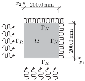
Figure 1: Cross-section of specimen

Figure 2: ISO fire curve

5.2 Example

Our model problem deals with a square concrete specimen of cross-section $200\times 200~{}{\rm mm^{2}}$, which is exposed to fire on the part $\Gamma_{R}$ of the boundary and insulated on the remaining portion $\Gamma_{N}$ (see Fig. 2). We assume that the ambient temperature in the vicinity of $\Gamma_{R}$ increases according to the ISO fire curve, ${\theta_{\infty}(t)=345\log(8t+1)+298.15}$, with $t$ given in minutes (see Fig. 2).

The uniform initial conditions are set to $\theta_{0}=298.15~{}{\rm K}$ and $P_{0}=2.7542\times 10^{3}~{}{\rm Pa}$ and the constants appearing in boundary conditions on $\Gamma_{R}$ are taken as $\alpha_{c}=25~{}{\rm{W\,m^{-2}K^{-1}}}$, $\beta_{c}=0.019~{}{\rm{m\,s^{-1}}}$, $P_{\infty}(t)=2.7542\times 10^{3}~{}{\rm Pa}$, $\sigma=5.67\times 10^{-8}~{}{\rm W\,m^{-2}K^{-4}}$ and $e=0.7$.

5.2.1 Material data for concrete at high temperatures

Physical quantity	Notation	Value	Dimension
Density of the solid microstructure	$\rho_{s}$	2400.0	${\rm kg\,m^{-3}}$
Specific heat of liquid phase	$C_{w}$	4181.0	${\rm J\,kg^{-1}K^{-1}}$
Enthalpy of dehydration	$h_{d}$	$2.4\times 10^{6}$	${\rm J\,kg^{-1}}$
Mass of cement per m3 of concrete	$c$	300.0	${\rm kg\,m^{-3}}$

Table 1: Material constants of concrete

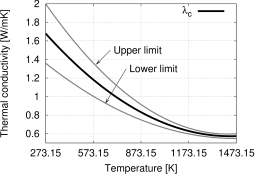
Basic material constants for concrete employed in this example appear in Table 1. Following [7], the thermal conductivity of concrete $\lambda_{c}$ can be bounded by lower $\lambda_{l}$ and upper $\lambda_{u}$ limit values defined by

$$\lambda_{l}(\theta) = 2.0-0.2451((\theta-273.15)/100.0)+0.0107((\theta-273.15)/100.0)^{2},$$

$$\lambda_{u}(\theta) = 1.36-0.136((\theta-273.15)/100.0)+0.0057((\theta-273.15)/100.0)^{2}$$

and is set to $\lambda_{c}(\theta)=(\lambda_{l}(\theta)+\lambda_{u}(\theta))/2$ in the results reported below.

Figure 3: Thermal conductivity of concrete

Figure 4: Permeability of concrete

Figure 5: Thermal capacity of solid skeleton

Figure 6: Mass of dehydrated water

The permeability of concrete $\kappa=\kappa(\theta,P)$ is adopted from [1, (12a)–(12b)] and the relative change in permeability $\kappa/\kappa_{0}$ [-], $\kappa_{0}=10^{-13}$ [ms^-1], is displayed in Fig. 4 as a function of temperature $\theta$ and relative humidity $RH$, defined as $RH(P,\theta)=P/P_{sat}(\theta)$, where $P_{sat}(\theta)$ is the vapor saturation pressure (see [4]).

The specific heat of solid matrix $C_{s}$ is considered in the form (cf. [4])

$$C_{s}(\theta)=900.0+80.0(\theta-273.15)/120.0-4.0((\theta-273.15)/120.0)^{2}.$$ (54)

The thermal capacity of solid skeleton is displayed in Fig. 6. Assuming that concrete is fully hydrated at room temperature, the mass of dehydrated water is given as [5]

$$w_{d}(\theta)=\left\{\begin{array}[]{rl}0.0&\text{for }\theta\leq 373.15\,\text{K},\\ 0.04c(\theta-373.15)/100.0&\text{for }373.15<\theta\leq 973.15\,\text{K},\\ 0.24c&\text{for }\theta>973.15\,\text{K},\end{array}\right.$$

see also Fig. 6 for an illustration. The temperature dependence of the enthalpy of evaporation $h_{\alpha}$ will be approximated by the Watson equation [6]

$$h_{\alpha}(\theta)=2.672\times 10^{5}(647.3-\theta)^{0.38}$$ (55)

provided $\theta\leq 647.3$ K. Note that for higher temperatures there is no liquid water in the pores and $h_{\alpha}(\theta)=0$.

The last comment concerns the sorption isotherms. For relative humidities $RH<0.96$ and $RH>1.04$, thermodynamics-based relations $w=\Phi(\theta,P)$ introduced in [1] are adopted. In the transition range, we employ the $C^{1}$-continuous cubic interpolation.

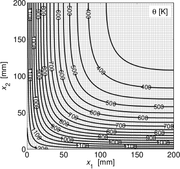
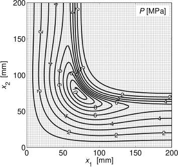
Figure 7: Temperature, pore pressure and water content distribution 30 min (left) and 60 min (right) after exposure to fire.

5.2.2 Results

The results presented in this section are obtained using an in-house MATLAB code and correspond to the uniform spatial discretization by $80\times 80$ square elements (without any adaptivity) and to the time step $\Delta t=5$ s. The distribution of individual fields at two characteristic times appears in Fig. 7.

We observe that the numerical model correctly reproduces the rapid heating of concrete specimen, accompanied by highly localized profile of water content distribution. Mainly the latter phenomenon, which is accurately resolved by the adopted fine grid, then contributes to the development of high values of pore pressure in the interior of the structure, leading to a potential threat to its stability during fire due to explosive spalling.

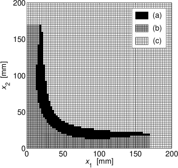
Figure 8: Spalling of concrete 40 min (left) and 60 min (right) after exposure to fire. Region (a) denotes elements failed due to spalling, (b) marks unstable elements and (c) stable part of the cross-section.

In order to assess this behavior more quantitatively, we adopt a conservative engineering approach and assume that the spalling of concrete occurs when the (appropriately reduced) pore pressure exceeds the temperature-dependent tensile strength of concrete. In particular, the spalling at $\mbox{\boldmath{$x$}}\in\Omega^{h}$ and time $t_{n}$ occurs when [5, Section 3.3]

$${\phi}P^{h}_{n}(\mbox{\boldmath{$x$}})\geq f_{t}\left(\theta^{h}_{n}(\mbox{\boldmath{$x$}})\right),$$ (56)

where $\phi$ is the porosity of concrete, $P^{h}_{n}$ and $\theta^{h}_{n}$ denote the finite element approximations of pore pressure and temperature for mesh size $h$ and the $n$-th time step and $f_{t}$ as a function of $\theta$ is provided by a piecewise linear relation [5, Section 4.4]

$$f_{t}(\theta)=f_{t0}\times\left\{\begin{array}[]{rl}1&\text{for }\theta\leq 373.15~{}\text{K},\\ (873.15-\theta)/500&\text{for }373.15~{}\text{K}<\theta\leq 823.15~{}\text{K},\\ (1473.15-\theta)/6500&\text{for }823.15~{}\text{K}<\theta\leq 1473.15~{}\text{K},\\ 0&\text{otherwise,}\end{array}\right.$$ (57)

where $f_{t0}$ designates the initial tensile strength of concrete.

The spatial distribution of the spalling damage for $\phi=0.1$ and $f_{t0}=2$ MPa appears in Fig. 8. Here, three different zones can be distinguished. The first region (a), highlighted in black color, corresponds to elements failed due to spalling damage as predicted by the criterion (56) for the element center. The second zone (b) corresponds to the part of the structure in which the local strength is sufficiently high to sustain the pore pressure, but its stability is lost due the explosive spalling of the former region. Finally, the light gray zone (c) indicates the portion of the cross-section still capable of transmitting stresses due to mechanical loading, which is thereby responsible for the structural safety during fire.

References

• [1] Z.P. Bažant and W. Thonguthai, Pore pressure and drying of concrete at high temperature, Proc. ASCE J. Eng. Mech. Div. 104 (1978) 1058–1080.
• [2] D. Braess, Finite Elements. Theory, Fast Solvers, and Applications in Elasticity Theory, Cambridge University Press, Cambridge, NY, 2007.
• [3] J. Dalík, J. Daněček and J. Vala, Numerical Solution of the Kiessl Model, Appl. Math. 45 (2000) 3–17.
• [4] C.T. Davie, C.J. Pearce and N. Bicanic, Coupled heat and moisture transport in concrete at elevated temperatures - Effects of capillary pressure and adsorbed water, Numer. Heat Transfer Part A 49 (2006) 733–763.
• [5] M.B. Dwaikat, V.K.R. Kodur, Hydrothermal model for predicting fire-induced spalling in concrete structural systems. Fire Saf. J. 44 (2009) 425–434.
• [6] D. Gawin, C.E. Majorana and B.A. Schrefler, Numerical analysis of hygro-thermal behaviour and damage of concrete at high temperature, Mech. Cohes.-Frict. Mater. 4 (1999) 37–74.
• [7] Eurocode 2, General rules–structural fire design, in: prEN1992-1-2: design of concrete structures, Part 1–2, Comité Europeén de Normalisation (CEN), Brussels, 2004.
• [8] K. Kiessl, Kapillarer und dampfförmiger Feuchtetransport in mehrshichtigen Bauteilen. Rechnerische Erfassung und bauhysikalische Anwendung. Dissertation. Universität Essen, 1983.
• [9] A. Kufner, A.-M. Sändig, Some Aplications of Weighted Sobolev Spaces, Teubner-Texte zur Mathematik, Band 100, Leipzig 1987.
• [10] V.G. Maz’ya, J. Rossmann, Weighted Lpsubscript𝐿𝑝L_{p} estimates of solutions to boundary value problems for second order elliptic systems in polyhedral domains. ZAMM Z. Angew. Math. Mech. 83 (2003), no. 7, 435–467.
• [11] J. Nečas, Introduction to the theory of nonlinear elliptic equations, Teubner-Texte zur Mathematik, Leipzig, 1983.
• [12] J. Ožbolt, G. Periškic, H.W. Reinhardt, R. Eligehausen, Numerical analysis of spalling of concrete cover at high temperature. Comput. Concr. 5 (2008), no. 4, 279–293.
• [13] R. Tenchev, L.Y. Li and J.A. Purkiss, Finite element analysis of coupled heat and moisture transfer in concrete subjected to fire. Numer. Heat Transfer Part A 39 (2001) 685–710.