Robust linear least squares regression

Abstract

We consider the problem of robustly predicting as well as the best linear combination of $d$ given functions in least squares regression, and variants of this problem including constraints on the parameters of the linear combination. For the ridge estimator and the ordinary least squares estimator, and their variants, we provide new risk bounds of order $d/n$ without logarithmic factor unlike some standard results, where $n$ is the size of the training data. We also provide a new estimator with better deviations in the presence of heavy-tailed noise. It is based on truncating differences of losses in a min–max framework and satisfies a $d/n$ risk bound both in expectation and in deviations. The key common surprising factor of these results is the absence of exponential moment condition on the output distribution while achieving exponential deviations. All risk bounds are obtained through a PAC-Bayesian analysis on truncated differences of losses. Experimental results strongly back up our truncated min–max estimator.

and

1 Introduction.

Our statistical task.

Let $Z_{1}=(X_{1},Y_{1}),\ldots,Z_{n}=(X_{n},Y_{n})$ be $n\geq 2$ pairs of input–output and assume that each pair has been independently drawn from the same unknown distribution $P$. Let $\mathcal{X}$ denote the input space and let the output space be the set of real numbers $\mathbb{R}$, so that $P$ is a probability distribution on the product space $\mathcal{Z}\triangleq\mathcal{X}\times\mathbb{R}$. The target of learning algorithms is to predict the output $Y$ associated with an input $X$ for pairs $Z=(X,Y)$ drawn from the distribution $P$. The quality of a (prediction) function $f\dvtx\mathcal{X}\rightarrow\mathbb{R}$ is measured by the least squares risk:

$$R(f)\triangleq{\mathbb{E}}_{Z\sim P}\{[Y-f(X)]^{2}\}.$$

Through the paper, we assume that the output and all the prediction functions we consider are square integrable. Let $\Theta$ be a closed convex set of $\mathbb{R}^{d}$, and $\varphi_{1},\ldots,\varphi_{d}$ be $d$ prediction functions. Consider the regression model

$$\mathcal{F}=\Biggl{\{}f_{\theta}=\sum_{j=1}^{d}\theta_{j}\varphi_{j};(\theta_{1},\ldots,\theta_{d})\in\Theta\Biggr{\}}.$$

The best function $f^{*}$ in $\mathcal{F}$ is defined by

$$f^{*}=\sum_{j=1}^{d}\theta^{*}_{j}\varphi_{j}\in\mathop{\arg\min}_{f\in\mathcal{F}}R(f).$$

Such a function always exists but is not necessarily unique. Besides, it is unknown since the probability generating the data is unknown.

We will study the problem of predicting (at least) as well as function $f^{*}$. In other words, we want to deduce from the observations $Z_{1},\ldots,Z_{n}$ a function $\hat{f}$ having with high probability a risk bounded by the minimal risk $R(f^{*})$ on $\mathcal{F}$ plus a small remainder term, which is typically of order $d/n$ up to a possible logarithmic factor. Except in particular settings (e.g., $\Theta$ is a simplex and $d\geq\sqrt{n}$), it is known that the convergence rate $d/n$ cannot be improved in a minimax sense (see Tsy03 and Yan01b for related results).

More formally, the target of the paper is to develop estimators $\hat{f}$ for which the excess risk is controlled in deviations, that is, such that for an appropriate constant $\kappa>0$, for any $\varepsilon>0$, with probability at least $1-\varepsilon$,

$$R(\hat{f})-R(f^{*})\leq\frac{\kappa[d+\log(\varepsilon^{-1})]}{n}.$$ (1)

Note that by integrating the deviations [using the identity $\mathbb{E}(W)=\break\int_{0}^{+\infty}\mathbb{P}(W>t)\,dt$ which holds true for any non-negative random variable $W$], inequality (1) implies

$$\mathbb{E}R(\hat{f})-R(f^{*})\leq\frac{\kappa(d+1)}{n}.$$ (2)

In this work, we do not assume that the function

$$f^{(\mathrm{reg})}\dvtx x\mapsto\mathbb{E}[Y|X=x],$$

which minimizes the risk $R$ among all possible measurable functions, belongs to the model $\mathcal{F}$. So we might have $f^{*}\neq f^{(\mathrm{reg})}$ and in this case, bounds of the form

$$\mathbb{E}R(\hat{f})-R\bigl{(}f^{(\mathrm{reg})}\bigr{)}\leq C\bigl{[}R(f^{*})-R\bigl{(}f^{(\mathrm{reg})}\bigr{)}\bigr{]}+\kappa\frac{d}{n}$$ (3)

with a constant $C$ larger than $1$, do not even ensure that $\mathbb{E}R(\hat{f})$ tends to $R(f^{*})$ when $n$ goes to infinity. These kinds of bounds with $C>1$ have been developed to analyze nonparametric estimators using linear approximation spaces, in which case the dimension $d$ is a function of $n$ chosen so that the bias term $R(f^{*})-R(f^{(\mathrm{reg})})$ has the order $d/n$ of the estimation term (see Bar00 , Gyo04 , Sau10 and references within). Here we intend to assess the generalization ability of the estimator even when the model is misspecified [namely, when $R(f^{*})>R(f^{(\mathrm{reg})})$]. Moreover, we do not assume either that $Y-f^{(\mathrm{reg})}(X)$ and $X$ are independent or that $Y$ has a subexponential tail distribution: for the moment, we just assume that $Y-f^{*}(X)$ admits a finite second-order moment in order that the risk of $f^{*}$ is finite.

Several risk bounds with $C=1$ can be found in the literature. A survey on these bounds is given in AudCat210 , Section 1. Let us mention here the closest bound to what we are looking for. From the work of Birgé and Massart BirMas98 , we may derive the following risk bound for the empirical risk minimizer on a $L^{\infty}$ ball (see Appendix B of AudCat210 ).

Theorem 1.1

Assume that $\mathcal{F}$ has a diameter $H$ for $L^{\infty}$-norm, that is, for any $f_{1},f_{2}$ in $\mathcal{F}$, ${\sup_{x\in\mathcal{X}}}|f_{1}(x)-f_{2}(x)|\leq H$ and there exists a function $f_{0}\in\mathcal{F}$ satisfying the exponential moment condition

$$\mbox{for any }x\in\mathcal{X}\qquad\mathbb{E}\{\exp[A^{-1}|Y-f_{0}(X)|]|X=x\}\leq M$$ (4)

for some positive constants $A$ and $M$. Let

$$\tilde{B}=\inf_{\phi_{1},\ldots,\phi_{d}}\sup_{\theta\in\mathbb{R}^{d}-\{0\}}\frac{\|{\sum_{j=1}^{d}\theta_{j}\phi_{j}}\|_{\infty}^{2}}{\|\theta\|_{\infty}^{2}},$$

where the infimum is taken with respect to all possible orthonormal bases of $\mathcal{F}$ for the dot product $(f_{1},f_{2})\mapsto\mathbb{E}[f_{1}(X)f_{2}(X)]$ (when the set $\mathcal{F}$ admits no basis with exactly $d$ functions, we set $\tilde{B}=+\infty$). Then the empirical risk minimizer satisfies for any $\varepsilon>0$, with probability at least $1-\varepsilon$,

$$R\bigl{(}\hat{f}^{(\mathrm{erm})}\bigr{)}-R(f^{*})\leq\kappa(A^{2}+H^{2})\frac{d\log[2+(\tilde{B}/n)\wedge(n/d)]+\log(\varepsilon^{-1})}{n},$$

where $\kappa$ is a positive constant depending only on $M$.

The theorem gives exponential deviation inequalities of order at worse $d\log(n/d)/{n}$ and, asymptotically, when $n$ goes to infinity, of order $d/n$. This work will provide similar results under weaker assumptions on the output distribution.

Notation. When $\Theta=\mathbb{R}^{d}$, the function $f^{*}$ and the space $\mathcal{F}$ will be written $f^{*}_{\mathrm{lin}}$ and $\mathcal{F}_{\mathrm{lin}}$ to emphasize that $\mathcal{F}$ is the whole linear space spanned by $\varphi_{1},\ldots,\varphi_{d}$:

$$\mathcal{F}_{\mathrm{lin}}=\operatorname{span}\{\varphi_{1},\ldots,\varphi_{d}\}\quad\mbox{and}\quad f^{*}_{\mathrm{lin}}\in\mathop{\arg\min}_{f\in\mathcal{F}_{\mathrm{lin}}}R(f).$$

The Euclidean norm will simply be written as $\|\cdot\|$, and $\langle\cdot,\cdot\rangle$ will be its associated inner product. We will consider the vector valued function $\varphi\dvtx\mathcal{X}\rightarrow\mathbb{R}^{d}$ defined by $\varphi(X)=[\varphi_{k}(X)]_{k=1}^{d}$, so that for any $\theta\in\Theta$, we have

$$f_{\theta}(X)=\langle\theta,\varphi(X)\rangle.$$

The Gram matrix is the $d\times d$-matrix $Q=\mathbb{E}[\varphi(X)\varphi(X)^{T}]$. The empirical risk of a function $f$ is $r(f)=\frac{1}{n}\sum_{i=1}^{n}[f(X_{i})-Y_{i}]^{2}$ and for $\lambda\geq 0$, the ridge regression estimator on $\mathcal{F}$ is defined by $\hat{f}^{(\mathrm{ridge})}=f_{\hat{\theta}^{(\mathrm{ridge})}}$ with

$$\hat{\theta}^{(\mathrm{ridge})}\in\mathop{\arg\min}_{\theta\in\Theta}\{r(f_{\theta})+\lambda\|\theta\|^{2}\},$$

where $\lambda$ is some non-negative real parameter. In the case when $\lambda=0$, the ridge regression $\hat{f}^{(\mathrm{ridge})}$ is nothing but the empirical risk minimizer $\hat{f}^{(\mathrm{erm})}$. Besides, the empirical risk minimizer when $\Theta=\mathbb{R}^{d}$ is also called the ordinary least squares estimator, and will be denoted by $\hat{f}^{(\mathrm{ols})}$.

In the same way, we introduce the optimal ridge function optimizing the expected ridge risk: $\tilde{f}=f_{\tilde{\theta}}$ with

$$\tilde{\theta}\in\mathop{\arg\min}_{\theta\in\Theta}\{R(f_{\theta})+\lambda\|\theta\|^{2}\}.$$ (5)

Finally, let $Q_{\lambda}=Q+\lambda I$ be the ridge regularization of $Q$, where $I$ is the identity matrix.

Why should we be interested in this task?

There are four main reasons. First, we intend to provide a nonasymptotic analysis of the parametric linear least squares method. Second, the task is central in nonparametric estimation for linear approximation spaces (piecewise polynomials based on a regular partition, wavelet expansions, trigonometric polynomials$\ldots$).

Third, it naturally arises in two-stage model selection. Precisely, when facing the data, the statistician often has to choose several models which are likely to be relevant for the task. These models can be of similar structure (like embedded balls of functional spaces) or, on the contrary, of a very different nature (e.g., based on kernels, splines, wavelets or on a parametric approach). For each of these models, we assume that we have a learning scheme which produces a “good” prediction function in the sense that it predicts as well as the best function of the model up to some small additive term. Then the question is to decide on how we use or combine/aggregate these schemes. One possible answer is to split the data into two groups, use the first group to train the prediction function associated with each model, and finally use the second group to build a prediction function which is as good as (i) the best of the previously learned prediction functions, (ii) the best convex combination of these functions or (iii) the best linear combination of these functions. This point of view has been introduced by Nemirovski in Nem98 and optimal rates of aggregation are given in Tsy03 and the references within. This paper focuses more on the linear aggregation task [even if (ii) enters in our setting], assuming implicitly here that the models are given in advance and are beyond our control and that the goal is to combine them appropriately.

Finally, in practice, the noise distribution often departs from the normal distribution. In particular, it can exhibit much heavier tails, and consequently induce highly non-Gaussian residuals. It is then natural to ask whether classical estimators such as the ridge regression and the ordinary least squares estimator are sensitive to this type of noise, and whether we can design more robust estimators.

Outline and contributions.

Section 2 provides a new analysis of the ridge estimator and the ordinary least squares estimator, and their variants. Theorem 2.1 provides an asymptotic result for the ridge estimator, while Theorem 2.2 gives a nonasymptotic risk bound for the empirical risk minimizer, which is complementary to the theorems put in the survey section. In particular, the result has the benefit to hold for the ordinary least squares estimator and for heavy-tailed outputs. We show quantitatively that the ridge penalty leads to an implicit reduction of the input space dimension. Section 3 shows a nonasymptotic $d/n$ exponential deviation risk bound under weak moment conditions on the output $Y$ and on the $d$-dimensional input representation $\varphi(X)$.

The main contribution of this paper is to show through a PAC-Bayesian analysis on truncated differences of losses that the output distribution does not need to have bounded conditional exponential moments in order for the excess risk of appropriate estimators to concentrate exponentially. Our results tend to say that truncation leads to more robust algorithms. Local robustness to contamination is usually invoked to advocate the removal of outliers, claiming that estimators should be made insensitive to small amounts of spurious data. Our work leads to a different theoretical explanation. The observed points having unusually large outputs when compared with the (empirical) variance should be down-weighted in the estimation of the mean, since they contain less information than noise. In short, huge outputs should be truncated because of their low signal-to-noise ratio.

2 Ridge regression and empirical risk minimization.

We recall the definition

$$\mathcal{F}=\Biggl{\{}f_{\theta}=\sum_{j=1}^{d}\theta_{j}\varphi_{j};(\theta_{1},\ldots,\theta_{d})\in\Theta\Biggr{\}},$$

where $\Theta$ is a closed convex set, not necessarily bounded (so that $\Theta=\mathbb{R}^{d}$ is allowed). In this section we provide exponential deviation inequalities for the empirical risk minimizer and the ridge regression estimator on $\mathcal{F}$ under weak conditions on the tail of the output distribution.

The most general theorem which can be obtained from the route followed in this section is Theorem 1.5 of the supplementary material AudCat11supp . It is expressed in terms of a series of empirical bounds. The first deduction we can make from this technical result is of an asymptotic nature. It is stated under weak hypotheses, taking advantage of the weak law of large numbers.

Theorem 2.1

For $\lambda\geq 0$, let $\tilde{f}$ be its associated optimal ridge function [see (5)]. Let us assume that

$$\mathbb{E}[\|\varphi(X)\|^{4}]<+\infty$$ (6)

and

$$\mathbb{E}\{\|\varphi(X)\|^{2}[\tilde{f}(X)-Y]^{2}\}<+\infty.$$ (7)

Let $\nu_{1}>\cdots>\nu_{d}$ be the eigenvalues of the Gram matrix $Q=\mathbb{E}[\varphi(X)\varphi(X)^{T}]$, and let $Q_{\lambda}=Q+\lambda I$ be the ridge regularization of $Q$. Let us define the effective ridge dimension

$$D=\sum_{i=1}^{d}\frac{\nu_{i}}{\nu_{i}+\lambda}\mathbh{1}(\nu_{i}>0)=\operatorname{Tr}[(Q+\lambda I)^{-1}Q]=\mathbb{E}[\|Q_{\lambda}^{-1/2}\varphi(X)\|^{2}].$$

When $\lambda=0$, $D$ is equal to the rank of $Q$ and is otherwise smaller. For any $\varepsilon>0$, there is $n_{\varepsilon}$, such that for any $n\geq n_{\varepsilon}$, with probability at least $1-\varepsilon$,

$$R\bigl{(}\hat{f}^{(\mathrm{ridge})}\bigr{)}+\lambda\bigl{\|}\hat{\theta}^{(\mathrm{ridge})}\bigr{\|}^{2}$$

$$\qquad\leq\min_{\theta\in\Theta}\{R(f_{\theta})+\lambda\|\theta\|^{2}\}$$

$$\qquad\quad{}+\frac{30\mathbb{E}\{\|Q_{\lambda}^{-1/2}\varphi(X)\|^{2}[\tilde{f}(X)-Y]^{2}\}}{\mathbb{E}\{\|Q_{\lambda}^{-1/2}\varphi(X)\|^{2}\}}\frac{D}{n}$$

$$\qquad\quad{}+1\mbox{,}000\sup_{v\in\mathbb{R}^{d}}\frac{\mathbb{E}[\langle v,\varphi(X)\rangle^{2}[\tilde{f}(X)-Y]^{2}]}{\mathbb{E}(\langle v,\varphi(X)\rangle^{2})+\lambda\|v\|^{2}}\frac{\log(3\varepsilon^{-1})}{n}$$

$$\qquad\leq\min_{\theta\in\Theta}\{R(f_{\theta})+\lambda\|\theta\|^{2}\}$$

$$\qquad\quad{}+\operatorname{ess}\sup\mathbb{E}\{[Y-\tilde{f}(X)]^{2}|X\}\frac{30D+1\mbox{,}000\log(3\varepsilon^{-1})}{n}.$$

See Section 1 of the supplementary material AudCat11supp .

This theorem shows that the ordinary least squares estimator (obtained when $\Theta=\mathbb{R}^{d}$ and $\lambda=0$), as well as the empirical risk minimizer on any closed convex set, asymptotically reaches a $d/n$ speed of convergence under very weak hypotheses. It shows also the regularization effect of the ridge regression. There emerges an effective dimension $D$, where the ridge penalty has a threshold effect on the eigenvalues of the Gram matrix.

Let us remark that the second inequality stated in the theorem provides a simplified bound which makes sense only when

$$\operatorname{ess}\sup\mathbb{E}\{[Y-\tilde{f}(X)]^{2}|X\}<+\infty$$

implying that $\|\tilde{f}-f^{(\mathrm{reg})}\|_{\infty}<+\infty$. We chose to state the first inequality as well, since it does not require such a tight relationship between $\tilde{f}$ and $f^{(\mathrm{reg})}$.

On the other hand, the weakness of this result is its asymptotic nature: $n_{\varepsilon}$ may be arbitrarily large under such weak hypotheses, and this happens even in the simplest case of the estimation of the mean of a real-valued random variable by its empirical mean [which is the case when $d=1$ and $\varphi(X)\equiv 1$].

Let us now give some nonasymptotic rate under stronger hypotheses and for the empirical risk minimizer (i.e., $\lambda=0$).

Theorem 2.2

Assume that $\mathbb{E}\{[Y-f^{*}(X)]^{4}\}<+\infty$ and

$$B=\sup_{f\in\operatorname{span}\{\varphi_{1},\ldots,\varphi_{d}\}-\{0\}}{\|f\|_{\infty}^{2}}/{\mathbb{E}[f(X)^{2}]}<+\infty.$$

Consider the (unique) empirical risk minimizer $\hat{f}^{(\mathrm{erm})}=f_{\hat{\theta}^{(\mathrm{erm})}}\dvtx x\mapsto\langle\hat{\theta}^{(\mathrm{erm})},\break\varphi(x)\rangle$ on $\mathcal{F}$ for which $\hat{\theta}^{(\mathrm{erm})}\in\operatorname{span}\{\varphi(X_{1}),\ldots,\varphi(X_{n})\}$. For any values of $\varepsilon$ and $n$ such that $2/n\leq\varepsilon\leq 1$ and

$$n>1280B^{2}\biggl{[}3Bd+\log(2/\varepsilon)+\frac{16B^{2}{d}^{2}}{n}\biggr{]}$$

with probability at least $1-\varepsilon$,

$$R\bigl{(}\hat{f}^{(\mathrm{erm})}\bigr{)}-R(f^{*})$$

(8)

$$\qquad\leq 1920B\sqrt{\mathbb{E}\{[Y-f^{*}(X)]^{4}\}}\biggl{[}\frac{3Bd+\log(2\varepsilon^{-1})}{n}+\biggl{(}\frac{4Bd}{n}\biggr{)}^{2}\biggr{]}.$$

See Section 1 of the supplementary material AudCat11supp .

It is quite surprising that the traditional assumption of uniform boundedness of the conditional exponential moments of the output can be replaced by a simple moment condition for reasonable confidence levels (i.e., $\varepsilon\geq 2/n$). For highest confidence levels, things are more tricky since we need to control with high probability a term of order $[r(f^{*})-R(f^{*})]d/n$ (see Theorem 1.6). The cost to pay to get the exponential deviations under only a fourth-order moment condition on the output is the appearance of the geometrical quantity $B$ as a multiplicative factor.

To better understand the quantity $B$, let us consider two cases. First, consider that the input is uniformly distributed on $\mathcal{X}=[0,1]$, and that the functions $\varphi_{1},\ldots,\varphi_{d}$ belong to the Fourier basis. Then the quantity $B$ behaves like a numerical constant. On the contrary, if we take $\varphi_{1},\ldots,\varphi_{d}$ as the first $d$ elements of a wavelet expansion, the more localized wavelets induce high values of $B$, and $B$ scales like $\sqrt{d}$, meaning that Theorem 2.2 fails to give a $d/n$-excess risk bound in this case. This limitation does not appear in Theorem 2.1.

To conclude, Theorem 2.2 is limited in at least four ways: it involves the quantity $B$, it applies only to uniformly bounded $\varphi(X)$, the output needs to have a fourth moment, and the confidence level should be as great as $\varepsilon\geq 2/n$. These limitations will be addressed in the next section by considering a more involved algorithm.

3 A min–max estimator for robust estimation.

This section provides an alternative to the empirical risk minimizer with nonasymptotic exponential risk deviations of order $d/n$ for any confidence level. Moreover, we will assume only a second-order moment condition on the output and cover the case of unbounded inputs, the requirement on $\varphi(X)$ being only a finite fourth-order moment. On the other hand, we assume here that the set $\Theta$ of the vectors of coefficients is bounded. The computability of the proposed estimator and numerical experiments are discussed at the end of the section.

3.1 The min–max estimator and its theoretical guarantee.

Let $\alpha>0$, $\lambda\geq 0$, and consider the truncation function:

$$\psi(x)=\cases{-\log(1-x+x^{2}/2),&\quad$0\leq x\leq 1$,\cr\log(2),&\quad$x\geq 1$,\cr-\psi(-x),&\quad$x\leq 0$.}$$

For any $\theta,\theta^{\prime}\in\Theta$, introduce

$$\mathcal{D}(\theta,\theta^{\prime})=n\alpha\lambda(\|\theta\|^{2}-\|\theta^{\prime}\|^{2})+\sum_{i=1}^{n}\psi\bigl{(}\alpha[Y_{i}-f_{\theta}(X_{i})]^{2}-\alpha[Y_{i}-f_{\theta^{\prime}}(X_{i})]^{2}\bigr{)}.$$

We recall that $\tilde{f}=f_{\tilde{\theta}}$ with $\tilde{\theta}\in\arg\min_{\theta\in\Theta}\{R(f_{\theta})+\lambda\|\theta\|^{2}\}$, and that the effective ridge dimension is defined as

$$D=\mathbb{E}[\|Q_{\lambda}^{-1/2}\varphi(X)\|^{2}]=\operatorname{Tr}[(Q+\lambda I)^{-1}Q]=\sum_{i=1}^{d}\frac{\nu_{i}}{\nu_{i}+\lambda}\mathbh{1}(\nu_{i}>0)\leq d,$$

where $\nu_{1}\geq\cdots\geq\nu_{d}$ are the eigenvalues of the Gram matrix $Q=\break\mathbb{E}[\varphi(X)\varphi(X)^{T}]$. Let us assume in this section that

$$\mathbb{E}\{[Y-\tilde{f}(X)]^{4}\}<+\infty,$$ (9)

and that for any $j\in\{1,\ldots,d\}$,

$$\mathbb{E}[\varphi_{j}(X)^{4}]<+\infty.$$ (10)

Define

$$\mathcal{S} = \{f\in\mathcal{F}_{\mathrm{lin}}\dvtx\mathbb{E}[f(X)^{2}]=1\},$$ (11)

$$\sigma = \sqrt{\mathbb{E}\{[Y-\tilde{f}(X)]^{2}\}}=\sqrt{R(\tilde{f})},$$ (12)

$$\chi = \max_{f\in\mathcal{S}}\sqrt{\mathbb{E}[f(X)^{4}]},$$ (13)

$$\kappa = \frac{\sqrt{\mathbb{E}\{[\varphi(X)^{T}Q_{\lambda}^{-1}\varphi(X)]^{2}\}}}{\mathbb{E}[\varphi(X)^{T}Q_{\lambda}^{-1}\varphi(X)]},$$ (14)

$$\kappa^{\prime} = \frac{\sqrt{\mathbb{E}\{[Y-\tilde{f}(X)]^{4}\}}}{\mathbb{E}\{[Y-\tilde{f}(X)]^{2}\}}=\frac{\sqrt{\mathbb{E}\{[Y-\tilde{f}(X)]^{4}\}}}{\sigma^{2}},$$ (15)

$$T = \max_{\theta\in\Theta,\theta^{\prime}\in\Theta}\sqrt{\lambda\|\theta-\theta^{\prime}\|^{2}+\mathbb{E}\{[f_{\theta}(X)-f_{\theta^{\prime}}(X)]^{2}\}}.$$ (16)

Theorem 3.1

Let us assume that (9) and (10) hold. For some numerical constants $c$ and $c^{\prime}$, for

$$n>c\kappa\chi D$$

by taking

$$\alpha=\frac{1}{2\chi[2\sqrt{\kappa^{\prime}}\sigma+\sqrt{\chi}T]^{2}}\biggl{(}1-\frac{c\kappa\chi D}{n}\biggr{)}$$ (17)

for any estimator $f_{\hat{\theta}}$ satisfying $\hat{\theta}\in\Theta$ a.s., for any $\varepsilon>0$ and any $\lambda\geq 0$, with probability at least $1-\varepsilon$, we have

$$R(f_{\hat{\theta}})+\lambda\|\hat{\theta}\|^{2} \leq \min_{\theta\in\Theta}\{R(f_{\theta})+\lambda\|\theta\|^{2}\}$$

$${}+\frac{1}{n\alpha}\Bigl{(}\max_{\theta_{1}\in\Theta}\mathcal{D}(\hat{\theta},\theta_{1})-\inf_{\theta\in{\Theta}}\max_{\theta_{1}\in{\Theta}}\mathcal{D}(\theta,\theta_{1})\Bigr{)}+\frac{c\kappa\kappa^{\prime}D\sigma^{2}}{n}$$

$${}+8\chi\biggl{(}\frac{\log(\varepsilon^{-1})}{n}+\frac{c^{\prime}\kappa^{2}D^{2}}{n^{2}}\biggr{)}\frac{[2\sqrt{\kappa^{\prime}}\sigma+\sqrt{\chi}T]^{2}}{1-{c\kappa\chi D}/{n}}.$$

See Section 2 of the supplementary material AudCat11supp .

By choosing an estimator such that

$$\max_{\theta_{1}\in\Theta}\mathcal{D}(\hat{\theta},\theta_{1})<\inf_{\theta\in{\Theta}}\max_{\theta_{1}\in{\Theta}}\mathcal{D}(\theta,\theta_{1})+\sigma^{2}\frac{D}{n},$$

Theorem 3.1 provides a nonasymptotic bound for the excess (ridge) risk with a $D/n$ convergence rate and an exponential tail even when neither the output $Y$ nor the input vector $\varphi(X)$ have exponential moments. This stronger nonasymptotic bound compared to the bounds of the previous section comes at the price of replacing the empirical risk minimizer by a more involved estimator. Section 3.3 provides a way of computing it approximately.

Theorem 3.1 requires a fourth-order moment condition on the output. In fact, one can replace (9) by the following second-order moment condition on the output: for any $j\in\{1,\ldots,d\}$,

$$\mathbb{E}\{\varphi_{j}(X)^{2}[Y-\tilde{f}(X)]^{2}\}<+\infty,$$

and still obtain a $D/n$ excess risk bound. This comes at the price of a more lengthy formula, where terms with $\kappa^{\prime}$ become terms involving the quantities $\max_{f\in\mathcal{S}}\mathbb{E}\{f(X)^{2}[Y-\tilde{f}(X)]^{2}\}$ and $\mathbb{E}\{\varphi(X)^{T}Q^{-1}\varphi(X)[Y-\tilde{f}(X)]^{2}\}$. (This can be seen by not using Cauchy–Schwarz’s inequality in (2.5) and (2.6) of the supplementary material AudCat11supp .)

3.2 The value of the uncentered kurtosis coefficients $\chi$ and $\kappa$.

We see that the speed of convergence of the excess risk in Theorem 3.1 (page 3.1) depends on three kurtosis-like coefficients, $\chi$, $\kappa$ and $\kappa^{\prime}$. The third, $\kappa^{\prime}$, is concerned with the noise, conceived as the difference between the observed output $Y$ and its best explanation $\tilde{f}(X)$ according to the ridge criterion. The aim of this section is to study the order of magnitude of the two other coefficients $\chi$ and $\kappa$, which are related to the design distribution,

$$\chi=\sup\{\mathbb{E}(\langle u,\varphi(X)\rangle^{4})^{1/2};u\in\mathbb{R}^{d},\mathbb{E}(\langle u,\varphi(X)\rangle^{2})\leq 1\}$$

and

$$\kappa=D^{-1}\mathbb{E}(\|Q_{\lambda}^{-1/2}\varphi(X)\|^{4})^{1/2}.$$

We will review a few typical situations.

3.2.1 Gaussian design.

Let us assume first that $\varphi(X)$ is a multivariate centered Gaussian random variable. In this case, its covariance matrix coincides with its Gram matrix $Q_{0}$ and can be written as

$$Q_{0}=U^{-1}\operatorname{Diag}(\nu_{i},i=1,\ldots,n)U,$$

where $U$ is an orthogonal matrix. Using $U$, we can introduce $W=UQ_{\lambda}^{-1/2}\varphi(X)$. It is also a Gaussian vector, with covariance $\operatorname{Diag}[\nu_{i}/(\lambda+\nu_{i}),i=1,\ldots,d]$. Moreover, since $U$ is orthogonal, $\|W\|=\|Q_{\lambda}^{-1/2}\varphi(X)\|$, and since $(W_{i},W_{j})$ are uncorrelated when $i\neq j$, they are independent, leading to

$$\mathbb{E}(\|Q_{\lambda}^{-1/2}\varphi(X)\|^{4}) = \mathbb{E}\Biggl{[}\Biggl{(}\sum_{i=1}^{d}W_{i}^{2}\Biggr{)}^{2}\Biggr{]}$$

$$= \sum_{i=1}^{d}\mathbb{E}(W_{i}^{4})+2\sum_{1\leq i<j\leq d}\mathbb{E}(W_{i}^{2})\mathbb{E}(W_{j}^{2})$$

$$= D^{2}+2D_{2},$$

where $D_{2}=\sum_{i=1}^{d}\frac{\nu_{i}^{2}}{(\lambda+\nu_{i})^{2}}$. Thus, in this case,

$$\kappa=\sqrt{1+2D_{2}D^{-2}}\leq\sqrt{1+\frac{2\nu_{1}}{(\lambda+\nu_{1})D}}\leq\sqrt{3}.$$

Moreover, as for any value of $u$, $\langle u,\varphi(X)\rangle$ is a Gaussian random variable, $\chi=\sqrt{3}$.

This situation arises in compressed sensing using random projections on Gaussian vectors. Specifically, assume that we want to recover a signal $f\in\mathbb{R}^{M}$ that we know to be well approximated by a linear combination of $d$ basis vectors $f_{1},\ldots,f_{d}$. We measure $n\ll M$ projections of the signal $f$ on i.i.d. $M$-dimensional standard normal random vectors $X_{1},\ldots,X_{n}\dvtx Y_{i}=\langle f,X_{i}\rangle$, $i=1,\ldots,n$. Then, recovering the coefficient $\theta_{1},\ldots,\theta_{d}$ such that $f=\sum_{j=1}^{d}\theta_{j}f_{j}$ is associated to the least squares regression problem, $Y\approx\sum_{j=1}^{d}\theta_{j}\varphi_{j}(X),$ with $\varphi_{j}(x)=\langle f_{j},x\rangle$, and $X$ having a $M$-dimensional standard normal distribution.

3.2.2 Independent design.

Let us study now the case when almost surely $\varphi_{1}(X)\equiv 1$ and $\varphi_{2}(X),\ldots,\varphi_{d}(X)$ are independent. To compute $\chi$, we can assume without loss of generality that $\varphi_{2}(X),\ldots,\varphi_{d}(X)$ are centered and of unit variance, since this renormalization is precisely the linear transformation that turns the Gram matrix into the identity matrix. Let us introduce

$$\chi_{*}=\max_{j=1,\ldots,d}\frac{\mathbb{E}[\varphi_{j}(X)^{4}]^{1/2}}{\mathbb{E}[\varphi_{j}(X)^{2}]}$$

with the convention $\frac{0}{0}=0$. A computation similar to the one made in the Gaussian case shows that

$$\kappa\leq\sqrt{1+(\chi_{*}^{2}-1)D_{2}D^{-2}}\leq\sqrt{1+\frac{(\chi_{*}^{2}-1)\nu_{1}}{(\lambda+\nu_{1})D}}\leq\chi_{*}.$$

Moreover, for any $u\in\mathbb{R}^{d}$ such that $\|u\|=1$,

$$\mathbb{E}(\langle u,\varphi(X)\rangle^{4}) = \sum_{i=1}^{d}u_{i}^{4}\mathbb{E}(\varphi_{i}(X)^{4})+6\sum_{1\leq i<j\leq d}u_{i}^{2}u_{j}^{2}\mathbb{E}[\varphi_{i}(X)^{2}]\mathbb{E}[\varphi_{j}(X)^{2}]$$

$${}+4\sum_{i=2}^{d}u_{1}u_{i}^{3}\mathbb{E}[\varphi_{i}(X)^{3}]$$

$$\leq \chi_{*}^{2}\sum_{i=1}^{d}u_{i}^{4}+6\sum_{i<j}u_{i}^{2}u_{j}^{2}+4\chi_{*}^{3/2}\sum_{i=2}^{d}|u_{1}u_{i}|^{3}$$

$$\leq \sup_{u\in\mathbb{R}_{+}^{d},\|u\|=1}(\chi_{*}^{2}-3)\sum_{i=1}^{d}u_{i}^{4}+3\Biggl{(}\sum_{i=1}^{d}u_{i}^{2}\Biggr{)}^{2}+4\chi_{*}^{3/2}u_{1}\sum_{i=2}^{d}u_{i}^{3}$$

$$\leq \frac{3^{3/2}}{4}\chi_{*}^{3/2}+\cases{\chi_{*}^{2},&\quad$\chi_{*}^{2}\geq 3$,\vspace*{2pt}\cr 3+\dfrac{\chi_{*}^{2}-3}{d},&\quad$1\leq\chi_{*}^{2}<3$.}$$

Thus, in this case,

$$\chi\leq\cases{\chi_{*}\biggl{(}1+\dfrac{3^{3/2}}{4\sqrt{\chi_{*}}}\biggr{)}^{1/2},&\quad$\chi_{*}\geq\sqrt{3}$,\vspace*{2pt}\cr\biggl{(}3+\dfrac{3^{3/2}}{4}\chi_{*}^{3/2}+\dfrac{\chi_{*}^{2}-3}{d}\biggr{)}^{1/2},&\quad$1\leq\chi_{*}<\sqrt{3}$.}$$

If, moreover, the random variables $\varphi_{2}(X),\ldots,\varphi_{d}(X)$ are not skewed, in the sense that $\mathbb{E}[\varphi_{j}(X)^{3}]=0$, $j=2,\ldots,d$, then

$$\cases{\chi=\chi_{*},&\quad$\chi_{*}\geq\sqrt{3}$,\vspace*{2pt}\cr\chi\leq\biggl{(}3+\dfrac{\chi_{*}^{2}-3}{d}\biggr{)}^{1/2},&\quad$1\leq\chi_{*}<\sqrt{3}$.}$$

3.2.3 Bounded design.

Let us assume now that the distribution of $\varphi(X)$ is almost surely bounded and nearly orthogonal. These hypotheses are suited to the study of regression in usual function bases, like the Fourier basis, wavelet bases, histograms or splines.

More precisely, let us assume that $\mathbb{P}(\|\varphi(X)\|\leq B)=1$ and that for some positive constant $A$ and any $u\in\mathbb{R}^{d}$,

$$\|u\|\leq A\mathbb{E}[\langle u,\varphi(X)\rangle^{2}]^{1/2}.$$

This appears as some stability property of the partial basis $\varphi_{j}$ with respect to the $\mathbb{L}_{2}$-norm, since it can also be written as

$$\sum_{j=1}^{d}u_{j}^{2}\leq A^{2}\mathbb{E}\Biggl{[}\Biggl{(}\sum_{j=1}^{d}u_{j}\varphi_{j}(X)\Biggr{)}^{2}\Biggr{]},\qquad u\in\mathbb{R}^{d}.$$

In terms of eigenvalues, $A^{-2}$ can be taken to be the lowest eigenvalue $\nu_{d}$ of the Gram matrix $Q$. The value of $A$ can also be deduced from a condition saying that $\varphi_{j}$ are nearly orthogonal in the sense that

$$\mathbb{E}[\varphi_{j}(X)^{2}]\geq 1\quad\mbox{and}\quad|\mathbb{E}[\varphi_{j}(X)\varphi_{k}(X)]|\leq\frac{1-A^{-2}}{d-1}.$$

In this situation, the chain of inequalities

$$\mathbb{E}[\langle u,\varphi(X)\rangle^{4}]\leq\|u\|^{2}B^{2}\mathbb{E}[\langle u,\varphi(X)\rangle^{2}]\leq A^{2}B^{2}\mathbb{E}[\langle u,\varphi(X)\rangle^{2}]^{2}$$

shows that $\chi\leq AB$. On the other hand,

$$\mathbb{E}[\|Q_{\lambda}^{-1/2}\varphi(X)\|^{4}]$$

$$\qquad=\mathbb{E}[\sup\{\langle u,\varphi(X)\rangle^{4};u\in\mathbb{R}^{d},\|Q_{\lambda}^{1/2}u\|\leq 1\}]$$

$$\qquad\leq\mathbb{E}[\sup\{\|u\|^{2}B^{2}\langle u,\varphi(X)\rangle^{2};\|Q^{1/2}_{\lambda}u\|\leq 1\}]$$

$$\qquad\leq\mathbb{E}[\sup\{(1+\lambda A^{2})^{-1}A^{2}B^{2}\|Q_{\lambda}^{1/2}u\|^{2}\langle u,\varphi(X)\rangle^{2};\|Q_{\lambda}^{1/2}u\|\leq 1\}]$$

$$\qquad\leq\frac{A^{2}B^{2}}{1+\lambda A^{2}}\mathbb{E}[\|Q_{\lambda}^{-1/2}\varphi(X)\|^{2}]=\frac{A^{2}B^{2}D}{1+\lambda A^{2}}$$

showing that $\kappa\leq\frac{AB}{\sqrt{(1+\lambda A^{2})D}}$.

For example, if $X$ is the uniform random variable on the unit interval and $\varphi_{j}$, $j=1,\ldots,d$, are any functions from the Fourier basis [meaning that they are of the form $\sqrt{2}\cos(2k\pi X)$ or $\sqrt{2}\sin(2k\pi X)$], then $A=1$ (because they form an orthogonal system) and $B\leq\sqrt{2d}$.

A localized basis like the evenly spaced histogram basis of the unit interval

$$\varphi_{j}(x)=\sqrt{d}\mathbh{1}\bigl{(}x\in[(j-1)/d,j/d[\bigr{)},\qquad j=1,\ldots,d,$$

will also be such that $A=1$ and $B=\sqrt{d}$. Similar computations could be made for other local bases, like wavelet bases.

Note that when $\chi$ is of order $\sqrt{d}$, and $\kappa$ and $\kappa^{\prime}$ of order $1$, Theo-rem 3.1 means that the excess risk of the min–max truncated estimator $\hat{f}$ is upper bounded by $Cd/n$ provided that $n\geq Cd^{2}$ for a large enough constant $C$.

3.2.4 Adaptive design planning.

Let us discuss the case when $X$ is some observed random variable whose distribution is only approximately known. Namely, let us assume that $(\varphi_{j})_{j=1}^{d}$ is some basis of functions in $\mathbb{L}_{2}[\tilde{\mathbb{P}}]$ with some known coefficient $\tilde{\chi}$, where $\tilde{\mathbb{P}}$ is an approximation of the true distribution of $X$ in the sense that the density of the true distribution $\mathbb{P}$ of $X$ with respect to the distribution $\tilde{\mathbb{P}}$ is in the range $(\eta^{-1},\eta)$. In this situation, the coefficient $\chi$ satisfies the inequality $\chi\leq\eta^{3/2}\tilde{\chi}$. Indeed,

$$\mathbb{E}_{X\sim\mathbb{P}}[\langle u,\varphi(X)\rangle^{4}] \leq \eta{\mathbb{E}}_{X\sim\tilde{\mathbb{P}}}[\langle u,\varphi(X)\rangle^{4}]$$

$$\leq \eta\tilde{\chi}^{2}{\mathbb{E}}_{X\sim\tilde{\mathbb{P}}}[\langle u,\varphi(X)\rangle^{2}]^{2}$$

$$\leq \eta^{3}\tilde{\chi}^{2}\mathbb{E}_{X\sim{\mathbb{P}}}[\langle u,\varphi(X)\rangle^{2}]^{2}.$$

In the same way, $\kappa\leq\eta^{7/2}\tilde{\kappa}$. Indeed,

$$\mathbb{E}[\sup\{\langle u,\varphi(X)\rangle^{4};\mathbb{E}(\langle u,\varphi(X)\rangle^{2})\leq 1\}]$$

$$\qquad\leq\eta\tilde{\mathbb{E}}[\sup\{\langle u,\varphi(X)\rangle^{4};\tilde{\mathbb{E}}(\langle u,\varphi(X)\rangle^{2})\leq\eta\}]$$

$$\qquad\leq\eta^{3}\tilde{\mathbb{E}}[\sup\{\langle u,\varphi(X)\rangle^{4};\tilde{\mathbb{E}}(\langle u,\varphi(X)\rangle^{2})\leq 1\}]$$

$$\qquad\leq\eta^{3}\tilde{\kappa}^{2}\tilde{\mathbb{E}}[\sup\{\langle u,\varphi(X)\rangle^{2};\tilde{\mathbb{E}}(\langle u,\varphi(X)\rangle^{2})\leq 1\}]^{2}$$

$$\qquad\leq\eta^{7}\tilde{\kappa}^{2}\mathbb{E}[\sup\{\langle u,\varphi(X)\rangle^{2};\mathbb{E}(\langle u,\varphi(X)\rangle^{2})\leq 1\}]^{2}.$$

Let us conclude this section with some scenario for the case when $X$ is a real-valued random variable. Let us consider the distribution function of $\tilde{\mathbb{P}}$,

$$\tilde{F}(x)=\tilde{\mathbb{P}}(X\leq x).$$

Then, if $\tilde{\mathbb{P}}$ has no atoms, the distribution of $\tilde{F}(X)$ would be uniform on $(0,1)$ if $X$ were distributed according to $\tilde{\mathbb{P}}$. In other words, $\tilde{\mathbb{P}}\circ\tilde{F}^{-1}=\mathbb{U}$, the uniform distribution on the unit interval. Starting from some suitable partial basis $(\varphi_{j})_{j=1}^{d}$ of $\mathbb{L}_{2}[(0,1),\mathbb{U}]$ like the ones discussed above, we can build a basis for our problem as

$$\tilde{\varphi}_{j}(X)=\varphi_{j}[\tilde{F}(X)].$$

Moreover, if $\mathbb{P}$ is absolutely continuous with respect to $\tilde{\mathbb{P}}$ with density $g$, then $\mathbb{P}\circ\tilde{F}^{-1}$ is absolutely continuous with respect to $\tilde{\mathbb{P}}\circ\tilde{F}^{-1}=\mathbb{U}$, with density $g\circ\tilde{F}^{-1}$, and, of course, the fact that $g$ takes values in $(\eta^{-1},\eta)$ implies the same property for $g\circ\tilde{F}^{-1}$. Thus, if $\tilde{\chi}$ and $\tilde{\kappa}$ are the coefficients corresponding to $\varphi_{j}(U)$ when $U$ is the uniform random variable on the unit interval, then the true coefficient $\chi$ [corresponding to $\tilde{\varphi}_{j}(X)$] will be such that $\chi\leq\eta^{3/2}\tilde{\chi}$ and $\kappa\leq\eta^{7/2}\tilde{\kappa}$.

3.3 Computation of the estimator.

For ease of description of the algorithm, we will write $X$ for $\varphi(X)$, which is equivalent to considering without loss of generality that the input space is $\mathbb{R}^{d}$ and that the functions $\varphi_{1},\ldots,\varphi_{d}$ are the coordinate functions. Therefore, the function $f_{\theta}$ maps an input $x$ to $\langle\theta,x\rangle$. Let us introduce

$$\overline{L}_{i}(\theta)=\alpha(\langle\theta,X_{i}\rangle-Y_{i})^{2}.$$

For any subset of indices $I\subset\{1,\ldots,n\}$, let us define

$$r_{I}(\theta)=\lambda\|\theta\|^{2}+\frac{1}{\alpha|I|}\sum_{i\in I}\overline{L}_{i}(\theta).$$

We suggest the following heuristics to compute an approximation of

$$\mathop{\arg\min}_{\theta\in\Theta}\sup_{\theta^{\prime}\in\Theta}\mathcal{D}(\theta,\theta^{\prime})\mbox{:}$$

• Start from $I_{1}=\{1,\ldots,n\}$ with the ordinary least squares estimate

  $$\hat{\theta}_{1}=\mathop{\arg\min}_{\mathbb{R}^{d}}r_{I_{1}}.$$

• At step number $k$, compute

  $$\hat{Q}_{k}=\frac{1}{|I_{k}|}\sum_{i\in I_{k}}X_{i}X_{i}^{T}.$$

• Consider the sets

  $$J_{k,1}(\eta)=\bigl{\{}i\in I_{k}\dvtx\overline{L}_{i}(\hat{\theta}_{k})X_{i}^{T}\hat{Q}_{k}^{-1}X_{i}\bigl{(}1+\sqrt{1+[\overline{L}_{i}(\hat{\theta}_{k})]^{-1}}\bigr{)}^{2}<\eta\bigr{\}},$$

  where $\hat{Q}_{k}^{-1}$ is the (pseudo-)inverse of the matrix $\hat{Q}_{k}$.

• Let us define

  $$\theta_{k,1}(\eta) = \mathop{\arg\min}_{\mathbb{R}^{d}}r_{J_{k,1}(\eta)},$$

  $$J_{k,2}(\eta) = \{i\in I_{k}\dvtx|\overline{L}_{i}(\theta_{k,1}(\eta))-\overline{L}_{i}(\hat{\theta}_{k})|\leq 1\},$$

  $$\theta_{k,2}(\eta) = \mathop{\arg\min}_{\mathbb{R}^{d}}r_{J_{k,2}(\eta)},$$

  $$(\eta_{k},\ell_{k}) = \mathop{\arg\min}_{\eta\in\mathbb{R}_{+},\ell\in\{1,2\}}\max_{j=1,\ldots,k}\mathcal{D}(\theta_{k,\ell}(\eta),\hat{\theta}_{j}),$$

  $$I_{k+1} = J_{k,\ell_{k}}(\eta_{k}),$$

  $$\hat{\theta}_{k+1} = \theta_{k,\ell_{k}}(\eta_{k}).$$

• Stop when

  $$\max_{j=1,\ldots,k}\mathcal{D}(\hat{\theta}_{k+1},\hat{\theta}_{j})\geq 0,$$

  and set $\hat{\theta}=\hat{\theta}_{k}$ as the final estimator of $\tilde{\theta}$.

Note that there will be at most $n$ steps, since $I_{k+1}\varsubsetneq I_{k}$ and in practice much less in this iterative scheme. Let us give some justification for this proposal. Let us notice first that

$$\mathcal{D}(\theta+h,\theta)$$

$$\qquad=n\alpha\lambda(\|\theta+h\|^{2}-\|\theta\|^{2})$$

$$\qquad\quad{}+\sum_{i=1}^{n}\psi\bigl{(}\alpha[2\langle h,X_{i}\rangle(\langle\theta,X_{i}\rangle-Y_{i})+\langle h,X_{i}\rangle^{2}]\bigr{)}.$$

Hopefully, $\tilde{\theta}=\arg\min_{\theta\in\mathbb{R}^{d}}(R(f_{\theta})+\lambda\|\theta\|^{2})$ is in some small neighborhood of $\hat{\theta}_{k}$ already, according to the distance defined by $Q\simeq\hat{Q}_{k}$. So we may try to look for improvements of $\hat{\theta}_{k}$ by exploring neighborhoods of $\hat{\theta}_{k}$ of increasing sizes with respect to some approximation of the relevant norm $\|\theta\|_{Q}^{2}=\mathbb{E}[\langle\theta,X\rangle^{2}]$.

Since the truncation function $\psi$ is constant on $(-\infty,-1]$ and $[1,+\infty)$, the map $\theta\mapsto\mathcal{D}(\theta,\hat{\theta}_{k})$ induces a decomposition of the parameter space into cells corresponding to different sets $I$ of examples. Indeed, such a set $I$ is associated to the set $\mathcal{C}_{I}$ of $\theta$ such that $\overline{L}_{i}(\theta)-\overline{L}_{i}(\hat{\theta}_{k})<1$ if and only if $i\in I$. Although this may not be the case, we will do as if the map $\theta\mapsto\mathcal{D}(\theta,\hat{\theta}_{k})$ restricted to the cell $\mathcal{C}_{I}$ reached its minimum at some interior point of $\mathcal{C}_{I}$, and approximates this minimizer by the minimizer of $r_{I}$.

The idea is to remove first the examples which will become inactive in the closest cells to the current estimate $\hat{\theta}_{k}$. The cells for which the contribution of example number $i$ is constant are delimited by at most four parallel hyperplanes.

It is easy to see that the square of the inverse of the distance of $\hat{\theta}_{k}$ to the closest of these hyperplanes is equal to

$$\frac{1}{\alpha}X_{i}^{T}\hat{Q}_{k}^{-1}X_{i}\overline{L}_{i}(\hat{\theta}_{k})\Biggl{(}1+\sqrt{1+\frac{1}{\overline{L}_{i}(\hat{\theta}_{k})}}\Biggr{)}^{2}.$$

Indeed, this distance is the infimum of $\|\hat{Q}_{k}^{1/2}h\|$, where $h$ is a solution of

$$\langle h,X_{i}\rangle^{2}+2\langle h,X_{i}\rangle(\langle\hat{\theta}_{k},X_{i}\rangle-Y_{i})=\frac{1}{\alpha}.$$

It is computed by considering $h$ of the form $h=\xi\|\hat{Q}_{k}^{-1/2}X_{i}\|^{-1}\hat{Q}_{k}^{-1}X_{i}$ and solving an equation of order two in $\xi$.

This explains the proposed choice of $J_{k,1}(\eta)$. Then a first estimate $\theta_{k,1}(\eta)$ is computed on the basis of this reduced sample, and the sample is readjusted to $J_{k,2}(\eta)$ by checking which constraints are really activated in the computation of $\mathcal{D}(\theta_{k,1}(\eta),\hat{\theta}_{k})$. The estimated parameter is then readjusted, taking into account the readjusted sample (this could as a variant be iterated more than once). Now that we have some new candidates $\theta_{k,\ell}(\eta)$, we check the minimax property against them to elect $I_{k+1}$ and $\hat{\theta}_{k+1}$. Since we did not check the minimax property against the whole parameter set $\Theta=\mathbb{R}^{d}$, we have no theoretical warranty for this simplified algorithm. Nonetheless, similar computations to what we did could prove that we are close to solving $\min_{j=1,\ldots,k}R(f_{\hat{\theta}_{j}})$, since we checked the minimax property on the reduced parameter set $\{\hat{\theta}_{j},j=1,\ldots,k\}$. Thus, the proposed heuristics are capable of improving on the performance of the ordinary least squares estimator, while being guaranteed not to degrade its performance significantly.

3.4 Synthetic experiments.

In Section 3.4.1, we detail the different kinds of noises we work with. Then, Sections 3.4.2, 3.4.3 and 3.4.4 describe the three types of functional relationships between the input, the output and the noise involved in our experiments. A motivation for choosing these input–output distributions was the ability to compute exactly the excess risk, and thus to compare easily estimators. Section 3.4.5 provides details about the implementation, its computational efficiency and the main conclusions of the numerical experiments. Figures and tables are postponed to the Appendix.

3.4.1 Noise distributions.

In our experiments, we consider different types of noise that are centered and with unit variance:

• the standard Gaussian noise, $W\sim\mathcal{N}(0,1)$,

• a heavy-tailed noise defined by $W=\operatorname{sign}(V)/|V|^{1/q}$, with $V\sim\mathcal{N}(0,1)$, a standard Gaussian random variable and $q=2.01$ (the real number $q$ is taken strictly larger than $2$ as for $q=2$, the random variable $W$ would not admit a finite second moment).

• an asymmetric heavy-tailed noise defined by

  $$W=\cases{|V|^{-1/q},&\quad if $V>0$,\vspace*{2pt}\cr-\dfrac{q}{q-1},&\quad otherwise,}$$

  with $q=2.01$ with $V\sim\mathcal{N}(0,1)$ a standard Gaussian random variable.

• a mixture of a Dirac random variable with a low-variance Gaussian random variable defined by, with probability $p$, $W=\sqrt{{(1-\rho)}/{p}}$, and with probability $1-p$, $W$ is drawn from

  $$\mathcal{N}\biggl{(}-\frac{\sqrt{p(1-\rho)}}{1-p},\frac{\rho}{1-p}-\frac{p(1-\rho)}{(1-p)^{2}}\biggr{)}.$$

  The parameter $\rho\in[p,1]$ characterizes the part of the variance of $W$ explained by the Gaussian part of the mixture. Note that this noise admits exponential moments, but for $n$ of order $1/p$, the Dirac part of the mixture generates low signal-to-noise points.

3.4.2 Independent normalized covariates [$\operatorname{INC}(n,d)$].

In INC$(n,d)$, we consider $\varphi(X)=X$, and the input–output pair is such that

$$Y=\langle\theta^{*},X\rangle+\sigma W,$$

where the components of $X$ are independent standard normal distributions, $\theta^{*}=(10,\ldots,10)^{T}\in\mathbb{R}^{d}$ and $\sigma=10$.

3.4.3 Highly correlated covariates [$\operatorname{HCC}(n,d)$].

In $\operatorname{HCC}(n,d)$, we consider $\varphi(X)=X$, and the input–output pair is such that

$$Y=\langle\theta^{*},X\rangle+\sigma W,$$

where $X$ is a multivariate centered normal Gaussian with covariance matrix $Q$ obtained by drawing a $(d,d)$-matrix $A$ of uniform random variables in $[0,1]$ and by computing $Q=AA^{T}$, $\theta^{*}=(10,\ldots,10)^{T}\in\mathbb{R}^{d}$ and $\sigma=10$. So the only difference with the setting of Section 3.4.2 is the correlation between the covariates.

3.4.4 Trigonometric series [$\operatorname{TS}(n,d)$].

Let $X$ be a uniform random variable on $[0,1]$. Let $d$ be an even number. In TS$(n,d)$, we consider

$$\varphi(X)=(\cos(2\pi X),\ldots,\cos(d\pi X),\sin(2\pi X),\ldots,\sin(d\pi X))^{T},$$

and the input–output pair is such that

$$Y=20X^{2}-10X-\tfrac 53+\sigma W$$

with $\sigma=10$. One can check that this implies

$$\theta^{*}=\biggl{(}\frac{20}{\pi^{2}},\ldots,\frac{20}{\pi^{2}({d}/2)^{2}},-\frac{10}{\pi},\ldots,-\frac{10}{\pi({d}/2)}\biggr{)}^{T}\in\mathbb{R}^{d}.$$

3.4.5 Experiments.

Choice of the parameters and implementation details.

The min–max truncated algorithm has two parameters $\alpha$ and $\lambda$. In the subsequent experiments, we set the ridge parameter $\lambda$ to the natural default choice for it: $\lambda=0$. For the truncation parameter $\alpha$, according to our analysis [see (17)], it roughly should be of order $1/\sigma^{2}$ up to kurtosis coefficients. By using the ordinary least squares estimator, we roughly estimate this value, and test values of $\alpha$ in a geometric grid (of $8$ points) around it (with ratio $3$). Cross-validation can be used to select the final $\alpha$. Nevertheless, it is computationally expensive and is significantly outperformed in our experiments by the following simple procedure: start with the smallest $\alpha$ in the geometric grid and increase it as long as $\hat{\theta}=\theta_{1}$, that is, as long as we stop at the end of the first iteration and output the empirical risk minimizer.

To compute $\theta_{k,1}(\eta)$ or $\theta_{k,2}(\eta)$, one needs to determine a least squares estimate (for a modified sample). To reduce the computational burden, we do not want to test all possible values of $\eta$ (note that there are at most $n$ values leading to different estimates). Our experiments show that testing only three levels of $\eta$ is sufficient. Precisely, we sort the quantity

$$\overline{L}_{i}(\hat{\theta}_{k})X_{i}^{T}\hat{Q}_{k}^{-1}X_{i}\bigl{(}1+\sqrt{1+[\overline{L}_{i}(\hat{\theta}_{k})]^{-1}}\bigr{)}^{2}$$

by decreasing order and consider $\eta$ being the first, $5$th and $25$th value of the ordered list. Overall, in our experiments, the computational complexity is approximately fifty times larger than the one of computing the ordinary least squares estimator.

Results.

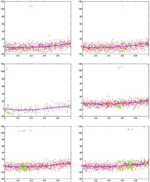
Figure 1: Circled points are the points of the training set generated several times from TS$(1\mbox{,}000,10)$ (with the mixture noise with $p=0.005$ and $\rho=0.4$) that are not taken into account in the min–max truncated estimator (to the extent that the estimator would not change by removing simultaneously all these points). The min–max truncated estimator $x\mapsto\hat{f}(x)$ appears in dash-dot line, while $x\mapsto\mathbb{E}(Y|X=x)$ is in solid line. In these six simulations, it outperforms the ordinary least squares estimator.

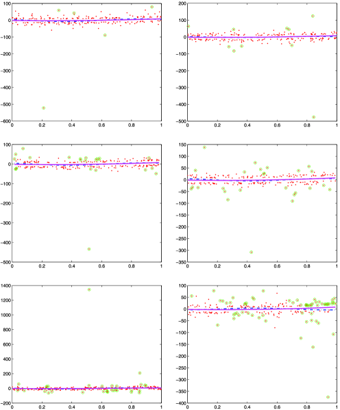
Figure 2: Circled points are the points of the training set generated several times from TS$(200,2)$ (with the heavy-tailed noise) that are not taken into account in the min–max truncated estimator (to the extent that the estimator would not change by removing these points). The min–max truncated estimator $x\mapsto\hat{f}(x)$ appears in dash-dot line, while $x\mapsto\mathbb{E}(Y|X=x)$ is in solid line. In these six simulations, it outperforms the ordinary least squares estimator. Note that in the last figure, it does not consider $64$ points among the $200$ training points.

The tables and figures have been gathered in the Appendix. Tables 1 and 2 give the results for the mixture noise. Tables 3, 4 and 5 provide the results for the heavy-tailed noise and the standard Gaussian noise. Each line of the tables has been obtained after 1,000 generations of the training set. These results show that the min–max truncated estimator is often equal to the ordinary least squares estimator $\hat{f}^{(\mathrm{ols})}$, while it ensures impressive consistent improvements when it differs from $\hat{f}^{(\mathrm{ols})}$. In this latter case, the number of points that are not considered in $\hat{f}$, that is, the number of points with low signal-to-noise ratio, varies a lot from $1$ to $150$ and is often of order $30$. Note that not only the points that we expect to be considered as outliers (i.e., very large output points) are erased, and that these points seem to be taken out by local groups: see Figures 1 and 2 in which the erased points are marked by surrounding circles.

Besides, the heavier the noise tail is (and also the larger the variance of the noise is), the more often the truncation modifies the initial ordinary least squares estimator, and the more improvements we get from the min–max truncated estimator, which also becomes much more robust than the ordinary least squares estimator (see the confidence intervals in the tables).

Finally, we have also tested more traditional methods in robust regression, namely, the M-estimators with Huber’s loss, $L_{1}$-loss and Tukey’s bisquare influence function, and also the least trimmed squares estimator, the S-estimator and the MM-estimator (see Rou84 , Yoh87 and the references within). These methods rely on diminishing the influence of points having “unreasonably” large residuals. They were developed to handle training sets containing true outliers, that is, points $(X,Y)$ not generated by the distribution $P$. This is not the case in our estimation framework. By overweighting points having reasonably small residuals, these methods are often biased even in settings where the noise is symmetric and the regression function $f^{(\mathrm{reg})}\dvtx x\mapsto\mathbb{E}[Y|X=x]$ belongs to $\mathcal{F}_{\mathrm{lin}}$ (i.e., $f^{(\mathrm{reg})}=f^{*}_{\mathrm{lin}}$), and also even when there is no noise (but $f^{(\mathrm{reg})}\notin f^{*}_{\mathrm{lin}}$).

The worst results were obtained by the $L_{1}$-loss, since estimating the (conditional) median is here really different from estimating the (conditional) mean. The MM-estimator and the M-estimators with Huber’s loss and Tukey’s bisquare influence function give good results as long as the signal-to-noise ratio is low. When the signal-to-noise ratio is high, a lack of consistency drastically appears in part of our simulations, showing that these methods are thus not suited for our estimation framework.

The S-estimator is almost consistently improving on the ordinary least squares estimator (in our simulations). However, when the signal-to-noise ratio is low (i.e., in the setting of the aforementioned simulations with $\sigma=10$), the improvements are much less significant than the ones of the min–max truncated estimator.

4 Main ideas of the proofs.

The goal of this section is to explain the key ingredients appearing in the proofs which both allow to obtain subexponential tails for the excess risk under a nonexponential moment assumption and get rid of the logarithmic factor in the excess risk bound.

4.1 Subexponential tails under a nonexponential moment assumption via truncation.

Let us start with the idea allowing us to prove exponential inequalities under just a moment assumption (instead of the traditional exponential moment assumption). To understand it, we can consider the (apparently) simplistic $1$-dimensional situation in which we have $\Theta=\mathbb{R}$ and the marginal distribution of $\varphi_{1}(X)$ is the Dirac distribution at $1$. In this case, the risk of the prediction function $f_{\theta}$ is $R(f_{\theta})=\mathbb{E}[(Y-\theta)^{2}]=\mathbb{E}[(Y-\mathbb{E}Y)^{2}]+(\mathbb{E}Y-\theta)^{2}$, so that the least squares regression problem boils down to the estimation of the mean of the output variable. If we only assume that $Y$ admits a finite second moment, say, $\mathbb{E}(Y^{2})\leq 1$, it is not clear whether for any $\varepsilon>0$, it is possible to find $\hat{\theta}$ such that, with probability at least $1-2\varepsilon$,

$$R(f_{\hat{\theta}})-R(f^{*})=\bigl{(}\mathbb{E}(Y)-\hat{\theta}\bigr{)}^{2}\leq c\frac{\log(\varepsilon^{-1})}{n}$$ (18)

for some numerical constant $c$. Indeed, from Chebyshev’s inequality, the trivial choice $\hat{\theta}=\frac{1}{n}\sum_{i=1}^{n}Y_{i}$ just satisfies, with probability at least $1-2\varepsilon$,

$$R(f_{\hat{\theta}})-R(f^{*})\leq\frac{1}{n\varepsilon},$$

which is far from the objective (18) for small confidence levels [consider $\varepsilon=\exp(-\sqrt{n})$, e.g.]. The key idea is thus to average (soft) truncated values of the outputs. This is performed by taking

$$\hat{\theta}=\frac{1}{n\lambda}\sum_{i=1}^{n}\log\biggl{(}1+\lambda Y_{i}+\frac{\lambda^{2}Y_{i}^{2}}{2}\biggr{)}$$

with $\lambda=\sqrt{\frac{2\log(\varepsilon^{-1})}{n}}$. Since we have

$$\log\mathbb{E}\exp(n\lambda\hat{\theta}) = n\log\biggl{(}1+\lambda\mathbb{E}(Y)+\frac{\lambda^{2}}{2}\mathbb{E}(Y^{2})\biggr{)}$$

$$\leq n\lambda\mathbb{E}(Y)+n\frac{\lambda^{2}}{2},$$

the exponential Chebyshev’s inequality guarantees that with probability at least $1-\varepsilon$, we have $n\lambda(\hat{\theta}-\mathbb{E}(Y))\leq n\lambda^{2}/2+\log(\varepsilon^{-1})$, hence,

$$\hat{\theta}-\mathbb{E}(Y)\leq\sqrt{\frac{2\log(\varepsilon^{-1})}{n}}.$$

Replacing $Y$ by $-Y$ in the previous argument, we obtain that, with probability at least $1-\varepsilon$, we have

$$n\lambda\Biggl{\{}\mathbb{E}(Y)+\frac{1}{n\lambda}\sum_{i=1}^{n}\log\biggl{(}1-\lambda Y_{i}+\frac{\lambda^{2}Y_{i}^{2}}{2}\biggr{)}\Biggr{\}}\leq n\frac{\lambda^{2}}{2}+\log(\varepsilon^{-1}).$$

Since $-\log(1+x+x^{2}/2)\leq\log(1-x+x^{2}/2)$, this implies $\mathbb{E}(Y)-\break\hat{\theta}\leq\sqrt{\frac{2\log(\varepsilon^{-1})}{n}}$. The two previous inequalities imply inequality (18) (for $c={2}$), showing that subexponential tails are achievable even when we only assume that the random variable admits a finite second moment (see Cat09 for more details on the robust estimation of the mean of a random variable).

4.2 Localized PAC-Bayesian inequalities to eliminate a logarithm factor.

Let us first recall that the Kullback–Leibler divergence between distributions $\rho$ and $\mu$ defined on $\mathcal{F}$ is

$$K(\rho,\mu)\triangleq\cases{\displaystyle{\mathbb{E}}_{f\sim\rho}\log\biggl{[}\frac{d\rho}{d\mu}(f)\biggr{]},&\quad if $\rho\ll\mu$,\vspace*{2pt}\cr+\infty,&\quad otherwise,}$$ (19)

where $\frac{d\rho}{d\mu}$ denotes as usual the density of $\rho$ w.r.t. $\mu$. For any real-valued (measurable) function $h$ defined on $\mathcal{F}$ such that $\int\exp[h(f)]\pi(df)<+\infty$, we define the distribution $\pi_{h}$ on $\mathcal{F}$ by its density:

$$\frac{d\pi_{h}}{d\pi}(f)=\frac{\exp[h(f)]}{\int\exp[h(f^{\prime})]\pi(df^{\prime})}.$$ (20)

The analysis of statistical inference generally relies on upper bounding the supremum of an empirical process $\chi$ indexed by the functions in a model $\mathcal{F}$. Concentration inequalities appear as a central tool to obtain these bounds. An alternative approach, called the PAC-Bayesian one, consists in using the entropic equality

$$\quad\mathbb{E}\exp\biggl{(}\sup_{\rho\in\mathcal{M}}\biggl{\{}\int\rho(df)\chi(f)-K(\rho,\pi^{\prime})\biggr{\}}\biggr{)}=\int\pi^{\prime}(df)\mathbb{E}\exp(\chi(f)),$$ (21)

where $\mathcal{M}$ is the set of probability distributions on $\mathcal{F}$.

Let $\check{r}\dvtx\mathcal{F}\rightarrow\mathbb{R}$ be an observable process such that, for any $f\in\mathcal{F}$, we have

$$\mathbb{E}\exp(\chi(f))\leq 1$$

for $\chi(f)=\lambda[R(f)-\check{r}(f)]$ and some $\lambda>0$. Then (21) leads to, for any $\varepsilon>0$, with probability at least $1-\varepsilon$, for any distribution $\rho$ on $\mathcal{F}$, we have

$$\int\rho(df)R(f)\leq\int\rho(df)\check{r}(f)+\frac{K(\rho,\pi^{\prime})+\log(\varepsilon^{-1})}{\lambda}.$$ (22)

The left-hand side quantity represents the expected risk with respect to the distribution $\rho$. To get the smallest upper bound on this quantity, a natural choice of the (posterior) distribution $\rho$ is obtained by minimizing the right-hand side, that is, by taking $\rho=\pi^{\prime}_{-\lambda\check{r}}$ [with the notation introduced in (20)]. This distribution concentrates on functions $f\in\mathcal{F}$ for which $\check{r}(f)$ is small. Without prior knowledge, one may want to choose a prior distribution $\pi^{\prime}=\pi$ which is rather “flat” (e.g., the one induced by the Lebesgue measure in the case of a model $\mathcal{F}$ defined by a bounded parameter set in some Euclidean space). Consequently, the Kullback–Leibler divergence $K(\rho,\pi^{\prime})$, which should be seen as the complexity term, might be excessively large.

To overcome the lack of prior information and the resulting high complexity term, one can alternatively use a more “localized” prior distribution. Here we use Gaussian distributions centered at the function of interest (e.g., the function $f^{*}$), and with covariance matrix proportional to the inverse of the Gram matrix $Q$. The idea of using PAC-Bayesian inequalities with Gaussian prior and posterior distributions goes back to Langford and Shawe-Taylor LanSha02 in the context of linear classification.

The detailed proofs of Theorems 2.1, 2.2 and 3.1 can be found in the supplementary material AudCat11supp .

Appendix: Experimental results for the min–max truncated estimator (Section 3.3)

==2pt Nb of Nb of iter. with Nb of iter. with $\bolds{\mathbb{E}R[(\hat{f}^{(\mathrm{ols})})|\hat{f}\!\neq\!\hat{f}^{(\mathrm{ols})}]}$ $\bolds{\mathbb{E}[R(\hat{f})|\hat{f}\!\neq\!\hat{f}^{(\mathrm{ols})}]}$ iterations $\bolds{R(\hat{f})\!\neq\!R(\hat{f}^{(\mathrm{ols})})}$ $\bolds{R(\hat{f})\!<\!R(\hat{f}^{(\mathrm{ols})})}$ $\bolds{\mathbb{E}R(\hat{f}^{(\mathrm{ols})})\!-\!R(f^{*})}$ $\bolds{\mathbb{E}R(\hat{f})\!-\!R(f^{*})}$ $\quad\bolds{-}\,\bolds{R(f^{*})}$ $\quad\bolds{-}\,\bolds{R(f^{*})}$ INC $(n\!=\!200,d\!=\!1$) $1\mbox{,}000$ $419$ $405$ $0.567$ $(\mbox{$\pm$}0.083)$ $0.178$ $(\mbox{$\pm$}0.025)$ $1.191$ $(\mbox{$\pm$}0.178)$ $0.262$ $(\mbox{$\pm$}0.052)$ INC $(n\!=\!200,d\!=\!2)$ $1\mbox{,}000$ $506$ $498$ $1.055$ $(\mbox{$\pm$}0.112)$ $0.271$ $(\mbox{$\pm$}0.030)$ $1.884$ $(\mbox{$\pm$}0.193)$ $0.334$ $(\mbox{$\pm$}0.050)$ HCC $(n\!=\!200,d\!=\!2)$ $1\mbox{,}000$ $502$ $494$ $1.045$ $(\mbox{$\pm$}0.103)$ $0.267$ $(\mbox{$\pm$}0.024)$ $1.866$ $(\mbox{$\pm$}0.174)$ $0.316$ $(\mbox{$\pm$}0.032)$ TS $(n\!=\!200,d\!=\!2)$ $1\mbox{,}000$ $561$ $554$ $1.069$ $(\mbox{$\pm$}0.089)$ $0.310$ $(\mbox{$\pm$}0.027)$ $1.720$ $(\mbox{$\pm$}0.132)$ $0.367$ $(\mbox{$\pm$}0.036)$ INC $(n\!=\!1\mbox{,}000,d\!=\!2)$ $1\mbox{,}000$ $402$ $392$ $0.204$ $(\mbox{$\pm$}0.015)$ $0.109$ $(\mbox{$\pm$}0.008)$ $0.316$ $(\mbox{$\pm$}0.029)$ $0.081$ $(\mbox{$\pm$}0.011)$ INC $(n\!=\!1\mbox{,}000,d\!=\!10)$ $1\mbox{,}000$ $950$ $946$ $1.030$ $(\mbox{$\pm$}0.041)$ $0.228$ $(\mbox{$\pm$}0.016)$ $1.051$ $(\mbox{$\pm$}0.042)$ $0.207$ $(\mbox{$\pm$}0.014)$ HCC $(n\!=\!1\mbox{,}000,d\!=\!10)$ $1\mbox{,}000$ $942$ $942$ $0.980$ $(\mbox{$\pm$}0.038)$ $0.222$ $(\mbox{$\pm$}0.015)$ $1.008$ $(\mbox{$\pm$}0.039)$ $0.203$ $(\mbox{$\pm$}0.015)$ TS $(n\!=\!1\mbox{,}000,d\!=\!10)$ $1\mbox{,}000$ $976$ $973$ $1.009$ $(\mbox{$\pm$}0.037)$ $0.228$ $(\mbox{$\pm$}0.017)$ $1.018$ $(\mbox{$\pm$}0.038)$ $0.217$ $(\mbox{$\pm$}0.016)$ INC $(n\!=\!2\mbox{,}000,d\!=\!2)$ $1\mbox{,}000$ $209$ $207$ $0.104$ $(\mbox{$\pm$}0.007)$ $0.078$ $(\mbox{$\pm$}0.005)$ $0.206$ $(\mbox{$\pm$}0.021)$ $0.082$ $(\mbox{$\pm$}0.012)$ HCC $(n\!=\!2\mbox{,}000,d\!=\!2)$ $1\mbox{,}000$ $184$ $183$ $0.099$ $(\mbox{$\pm$}0.007)$ $0.076$ $(\mbox{$\pm$}0.005)$ $0.196$ $(\mbox{$\pm$}0.023)$ $0.070$ $(\mbox{$\pm$}0.010)$ TS $(n\!=\!2\mbox{,}000,d\!=\!2)$ $1\mbox{,}000$ $172$ $171$ $0.101$ $(\mbox{$\pm$}0.007)$ $0.080$ $(\mbox{$\pm$}0.005)$ $0.206$ $(\mbox{$\pm$}0.020)$ $0.083$ $(\mbox{$\pm$}0.012)$ INC $(n\!=\!2\mbox{,}000,d\!=\!10)$ $1\mbox{,}000$ $669$ $669$ $0.510$ $(\mbox{$\pm$}0.018)$ $0.206$ $(\mbox{$\pm$}0.012)$ $0.572$ $(\mbox{$\pm$}0.023)$ $0.117$ $(\mbox{$\pm$}0.009)$ HCC $(n\!=\!2\mbox{,}000,d\!=\!10)$ $1\mbox{,}000$ $669$ $669$ $0.499$ $(\mbox{$\pm$}0.018)$ $0.207$ $(\mbox{$\pm$}0.013)$ $0.561$ $(\mbox{$\pm$}0.023)$ $0.125$ $(\mbox{$\pm$}0.011)$ TS $(n\!=\!2\mbox{,}000,d\!=\!10)$ $1\mbox{,}000$ $754$ $753$ $0.516$ $(\mbox{$\pm$}0.018)$ $0.195$ $(\mbox{$\pm$}0.013)$ $0.558$ $(\mbox{$\pm$}0.022)$ $0.131$ $(\mbox{$\pm$}0.011)$

Table 1: Comparison of the min–max truncated estimator $\hat{f}$ with the ordinary least squares estimator $\hat{f}^{(\mathrm{ols})}$ for the mixture noise (see Section 3.4.1) with $\rho=0.1$ and $p=0.005$. In parenthesis, the $95\%$-confidence intervals for the estimated quantities

==2pt Nb of Nb of iter. with Nb of iter. with $\bolds{\mathbb{E}R[(\hat{f}^{(\mathrm{ols})})|\hat{f}\!\neq\!\hat{f}^{(\mathrm{ols})}]}$ $\bolds{\mathbb{E}[R(\hat{f})|\hat{f}\!\neq\!\hat{f}^{(\mathrm{ols})}]}$ iterations $\bolds{R(\hat{f})\!\neq\!R(\hat{f}^{(\mathrm{ols})})}$ $\bolds{R(\hat{f})\!<\!R(\hat{f}^{(\mathrm{ols})})}$ $\bolds{\mathbb{E}R(\hat{f}^{(\mathrm{ols})})\!-\!R(f^{*})}$ $\bolds{\mathbb{E}R(\hat{f})\!-\!R(f^{*})}$ $\quad\bolds{-}\,\bolds{R(f^{*})}$ $\quad\bolds{-}\,\bolds{R(f^{*})}$ INC $(n\!=\!200,d\!=\!1)$ $1\mbox{,}000$ $234$ $211$ $0.551$ $(\mbox{$\pm$}0.063)$ $0.409$ $(\mbox{$\pm$}0.042)$ $1.211$ $(\mbox{$\pm$}0.210)$ $0.606$ $(\mbox{$\pm$}0.110)$ INC $(n\!=\!200,d\!=\!2)$ $1\mbox{,}000$ $195$ $186$ $1.046$ $(\mbox{$\pm$}0.088)$ $0.788$ $(\mbox{$\pm$}0.061)$ $2.174$ $(\mbox{$\pm$}0.293)$ $0.848$ $(\mbox{$\pm$}0.118)$ HCC $(n\!=\!200,d\!=\!2)$ $1\mbox{,}000$ $222$ $215$ $1.028$ $(\mbox{$\pm$}0.079)$ $0.748$ $(\mbox{$\pm$}0.051)$ $2.157$ $(\mbox{$\pm$}0.243)$ $0.897$ $(\mbox{$\pm$}0.112)$ TS $(n\!=\!200,d\!=\!2)$ $1\mbox{,}000$ $291$ $268$ $1.053$ $(\mbox{$\pm$}0.079)$ $0.805$ $(\mbox{$\pm$}0.058)$ $1.701$ $(\mbox{$\pm$}0.186)$ $0.851$ $(\mbox{$\pm$}0.093)$ INC $(n\!=\!1\mbox{,}000,d\!=\!2)$ $1\mbox{,}000$ $127$ $117$ $0.201$ $(\mbox{$\pm$}0.013)$ $0.181$ $(\mbox{$\pm$}0.012)$ $0.366$ $(\mbox{$\pm$}0.053)$ $0.207$ $(\mbox{$\pm$}0.035)$ INC $(n\!=\!1\mbox{,}000,d\!=\!10)$ $1\mbox{,}000$ $262$ $249$ $1.023$ $(\mbox{$\pm$}0.035)$ $0.902$ $(\mbox{$\pm$}0.030)$ $1.238$ $(\mbox{$\pm$}0.081)$ $0.777$ $(\mbox{$\pm$}0.054)$ HCC $(n\!=\!1\mbox{,}000,d\!=\!10)$ $1\mbox{,}000$ $201$ $192$ $0.991$ $(\mbox{$\pm$}0.033)$ $0.902$ $(\mbox{$\pm$}0.031)$ $1.235$ $(\mbox{$\pm$}0.088)$ $0.790$ $(\mbox{$\pm$}0.067)$ TS $(n\!=\!1\mbox{,}000,d\!=\!10)$ $1\mbox{,}000$ $171$ $162$ $1.009$ $(\mbox{$\pm$}0.033)$ $0.951$ $(\mbox{$\pm$}0.031)$ $1.166$ $(\mbox{$\pm$}0.098)$ $0.825$ $(\mbox{$\pm$}0.071)$ INC $(n\!=\!2\mbox{,}000,d\!=\!2)$ $1\mbox{,}000$ 0$80$ 0$77$ $0.105$ $(\mbox{$\pm$}0.007)$ $0.099$ $(\mbox{$\pm$}0.006)$ $0.214$ $(\mbox{$\pm$}0.042)$ $0.135$ $(\mbox{$\pm$}0.029)$ HCC $(n\!=\!2\mbox{,}000,d\!=\!2)$ $1\mbox{,}000$ 0$44$ 0$42$ $0.102$ $(\mbox{$\pm$}0.007)$ $0.099$ $(\mbox{$\pm$}0.007)$ $0.187$ $(\mbox{$\pm$}0.050)$ $0.120$ $(\mbox{$\pm$}0.034)$ TS $(n\!=\!2\mbox{,}000,d\!=\!2)$ $1\mbox{,}000$ 0$47$ 0$47$ $0.101$ $(\mbox{$\pm$}0.007)$ $0.099$ $(\mbox{$\pm$}0.007)$ $0.147$ $(\mbox{$\pm$}0.032)$ $0.103$ $(\mbox{$\pm$}0.026)$ INC $(n\!=\!2\mbox{,}000,d\!=\!10)$ $1\mbox{,}000$ $116$ $113$ $0.511$ $(\mbox{$\pm$}0.016)$ $0.491$ $(\mbox{$\pm$}0.016)$ $0.611$ $(\mbox{$\pm$}0.052)$ $0.437$ $(\mbox{$\pm$}0.042)$ HCC $(n\!=\!2\mbox{,}000,d\!=\!10)$ $1\mbox{,}000$ $110$ $105$ $0.500$ $(\mbox{$\pm$}0.016)$ $0.481$ $(\mbox{$\pm$}0.015)$ $0.602$ $(\mbox{$\pm$}0.056)$ $0.430$ $(\mbox{$\pm$}0.044)$ TS $(n\!=\!2\mbox{,}000,d\!=\!10)$ $1\mbox{,}000$ $101$ $98$ $0.511$ $(\mbox{$\pm$}0.016)$ $0.499$ $(\mbox{$\pm$}0.016)$ $0.601$ $(\mbox{$\pm$}0.054)$ $0.486$ $(\mbox{$\pm$}0.051)$

Table 2: Comparison of the min–max truncated estimator $\hat{f}$ with the ordinary least squares estimator $\hat{f}^{(\mathrm{ols})}$ for the mixture noise (see Section 3.4.1) with $\rho=0.4$ and $p=0.005$. In parenthesis, the $95\%$-confidence intervals for the estimated quantities

==2pt Nb of Nb of iter. with Nb of iter. with $\bolds{\mathbb{E}R[(\hat{f}^{(\mathrm{ols})})|\hat{f}\!\neq\!\hat{f}^{(\mathrm{ols})}]}$ $\bolds{\mathbb{E}[R(\hat{f})|\hat{f}\!\neq\!\hat{f}^{(\mathrm{ols})}]}$ iterations $\bolds{R(\hat{f})\!\neq\!R(\hat{f}^{(\mathrm{ols})})}$ $\bolds{R(\hat{f})\!<\!R(\hat{f}^{(\mathrm{ols})})}$ $\bolds{\mathbb{E}R(\hat{f}^{(\mathrm{ols})})\!-\!R(f^{*})}$ $\bolds{\mathbb{E}R(\hat{f})\!-\!R(f^{*})}$ $\quad\bolds{-}\,\bolds{R(f^{*})}$ $\quad\bolds{-}\,\bolds{R(f^{*})}$ INC $(n\!=\!200,d\!=\!1)$ 1,000 163 145 $7.72\mbox{ }(\mbox{$\pm$}3.46)$ $3.92\mbox{ }(\mbox{$\pm$}0.409)$ $30.52\mbox{ }(\mbox{$\pm$}20.8)$ 07.20 ($\pm$1.61) INC $(n\!=\!200,d\!=\!2)$ 1,000 104 098 $22.69\mbox{ }(\mbox{$\pm$}23.14)$ $19.18\mbox{ }(\mbox{$\pm$}23.09)$ $45.36\mbox{ }(\mbox{$\pm$}14.1)$ 11.63 ($\pm$2.19) HCC $(n\!=\!200,d\!=\!2)$ 1,000 120 117 $18.16\mbox{ }(\mbox{$\pm$}12.68)$ $8.07\mbox{ }(\mbox{$\pm$}0.718)$ $99.39\mbox{ }(\mbox{$\pm$}105)$ 15.34 ($\pm$4.41) TS $(n\!=\!200,d\!=\!2)$ 1,000 110 105 $43.89\mbox{ }(\mbox{$\pm$}63.79)$ $39.71\mbox{ }(\mbox{$\pm$}63.76)$ $48.55\mbox{ }(\mbox{$\pm$}18.4)$ 10.59 ($\pm$2.01) INC $(n\!=\!1\mbox{,}000,d\!=\!2)$ 1,000 104 100 $3.98\mbox{ }(\mbox{$\pm$}2.25)$ $1.78\mbox{ }(\mbox{$\pm$}0.128)$ $23.18\mbox{ }(\mbox{$\pm$}21.3)$ 02.03 ($\pm$0.56) INC $(n\!=\!1\mbox{,}000,d\!=\!10)$ 1,000 253 242 $16.36\mbox{ }(\mbox{$\pm$}5.10)$ $7.90\mbox{ }(\mbox{$\pm$}0.278)$ $41.25\mbox{ }(\mbox{$\pm$}19.8)$ 07.81 ($\pm$0.69) HCC $(n\!=\!1\mbox{,}000,d\!=\!10)$ 1,000 220 211 $13.57\mbox{ }(\mbox{$\pm$}1.93)$ $7.88\mbox{ }(\mbox{$\pm$}0.255)$ $33.13\mbox{ }(\mbox{$\pm$}8.2)$ 07.28 ($\pm$0.59) TS $(n\!=\!1\mbox{,}000,d\!=\!10)$ 1,000 214 211 $18.67\mbox{ }(\mbox{$\pm$}11.62)$ $13.79\mbox{ }(\mbox{$\pm$}11.52)$ $30.34\mbox{ }(\mbox{$\pm$}7.2)$ 07.53 ($\pm$0.58) INC $(n\!=\!2\mbox{,}000,d\!=\!2)$ 1,000 113 103 $1.56\mbox{ }(\mbox{$\pm$}0.41)$ $0.89\mbox{ }(\mbox{$\pm$}0.059)$ $6.74\mbox{ }(\mbox{$\pm$}3.4)$ 00.86 ($\pm$0.18) HCC $(n\!=\!2\mbox{,}000,d\!=\!2)$ 1,000 105 097 $1.66\mbox{ }(\mbox{$\pm$}0.43)$ $0.95\mbox{ }(\mbox{$\pm$}0.062)$ $7.87\mbox{ }(\mbox{$\pm$}3.8)$ 01.13 ($\pm$0.23) TS $(n\!=\!2\mbox{,}000,d\!=\!2)$ 1,000 101 095 $1.59\mbox{ }(\mbox{$\pm$}0.64)$ $0.88\mbox{ }(\mbox{$\pm$}0.058)$ $8.03\mbox{ }(\mbox{$\pm$}6.2)$ 01.04 ($\pm$0.22) INC $(n\!=\!2\mbox{,}000,d\!=\!10)$ 1,000 259 255 $8.77\mbox{ }(\mbox{$\pm$}4.02)$ $4.23\mbox{ }(\mbox{$\pm$}0.154)$ $21.54\mbox{ }(\mbox{$\pm$}15.4)$ 04.03 ($\pm$0.39) HCC $(n\!=\!2\mbox{,}000,d\!=\!10)$ 1,000 250 242 $6.98\mbox{ }(\mbox{$\pm$}1.17)$ $4.13\mbox{ }(\mbox{$\pm$}0.127)$ $15.35\mbox{ }(\mbox{$\pm$}4.5)$ 03.94 ($\pm$0.25) TS $(n\!=\!2\mbox{,}000,d\!=\!10)$ 1,000 238 233 $8.49\mbox{ }(\mbox{$\pm$}3.61)$ $5.95\mbox{ }(\mbox{$\pm$}3.486)$ $14.82\mbox{ }(\mbox{$\pm$}3.8)$ 04.17 ($\pm$0.30)

Table 3: Comparison of the min–max truncated estimator $\hat{f}$ with the ordinary least squares estimator $\hat{f}^{(\mathrm{ols})}$ with the heavy-tailed noise (see Section 3.4.1)

==2pt Nb of Nb of iter. with Nb of iter. with $\bolds{\mathbb{E}R[(\hat{f}^{(\mathrm{ols})})|\hat{f}\!\neq\!\hat{f}^{(\mathrm{ols})}]}$ $\bolds{\mathbb{E}[R(\hat{f})|\hat{f}\!\neq\!\hat{f}^{(\mathrm{ols})}]}$ iterations $\bolds{R(\hat{f})\!\neq\!R(\hat{f}^{(\mathrm{ols})})}$ $\bolds{R(\hat{f})\!<\!R(\hat{f}^{(\mathrm{ols})})}$ $\bolds{\mathbb{E}R(\hat{f}^{(\mathrm{ols})})\!-\!R(f^{*})}$ $\bolds{\mathbb{E}R(\hat{f})\!-\!R(f^{*})}$ $\quad\bolds{-}\,\bolds{R(f^{*})}$ $\quad\bolds{-}\,\bolds{R(f^{*})}$ INC $(n\!=\!200,d\!=\!1)$ 1,000 $87$ $77$ $5.49\mbox{ }(\mbox{$\pm$}3.07)$ $3.00\mbox{ }(\mbox{$\pm$}0.330)$ $35.44\mbox{ }(\mbox{$\pm$}34.7)$ 06.85 ($\pm$2.48) INC $(n\!=\!200,d\!=\!2)$ 1,000 $70$ $66$ $19.25\mbox{ }(\mbox{$\pm$}23.23)$ $17.4\mbox{ }(\mbox{$\pm$}23.2)$ $37.95\mbox{ }(\mbox{$\pm$}13.1)$ 11.05 ($\pm$2.87) HCC $(n\!=\!200,d\!=\!2)$ 1,000 $67$ $66$ $7.19\mbox{ }(\mbox{$\pm$}0.88)$ $5.81\mbox{ }(\mbox{$\pm$}0.397)$ $31.52\mbox{ }(\mbox{$\pm$}10.5)$ 10.87 ($\pm$2.64) TS $(n\!=\!200,d\!=\!2)$ 1,000 $76$ $68$ $39.80\mbox{ }(\mbox{$\pm$}64.09)$ $37.9\mbox{ }(\mbox{$\pm$}64.1)$ $34.28\mbox{ }(\mbox{$\pm$}14.8)$ 09.21 ($\pm$2.05) INC $(n\!=\!1\mbox{,}000,d\!=\!2)$ 1,000 $101$ $92$ $2.81\mbox{ }(\mbox{$\pm$}2.21)$ $1.31\mbox{ }(\mbox{$\pm$}0.106)$ $16.76\mbox{ }(\mbox{$\pm$}21.8)$ 01.88 ($\pm$0.69) INC $(n\!=\!1\mbox{,}000,d\!=\!10)$ 1,000 $211$ $195$ $10.71\mbox{ }(\mbox{$\pm$}4.53)$ $5.86\mbox{ }(\mbox{$\pm$}0.222)$ $29.00\mbox{ }(\mbox{$\pm$}21.3)$ 06.03 ($\pm$0.71) HCC $(n\!=\!1\mbox{,}000,d\!=\!10)$ 1,000 $197$ $185$ $8.67\mbox{ }(\mbox{$\pm$}1.16)$ $5.81\mbox{ }(\mbox{$\pm$}0.177)$ $20.31\mbox{ }(\mbox{$\pm$}5.59)$ 05.79 ($\pm$0.43) TS $(n\!=\!1\mbox{,}000,d\!=\!10)$ 1,000 $258$ $233$ $13.62\mbox{ }(\mbox{$\pm$}11.27)$ $11.3\mbox{ }(\mbox{$\pm$}11.2)$ $14.68\mbox{ }(\mbox{$\pm$}2.45)$ 05.60 ($\pm$0.36) INC $(n\!=\!2\mbox{,}000,d\!=\!2)$ 1,000 $106$ $92$ $1.04\mbox{ }(\mbox{$\pm$}0.37)$ $0.64\mbox{ }(\mbox{$\pm$}0.042)$ $4.54\mbox{ }(\mbox{$\pm$}3.45)$ 00.79 ($\pm$0.16) HCC $(n\!=\!2\mbox{,}000,d\!=\!2)$ 1,000 $99$ $90$ $0.90\mbox{ }(\mbox{$\pm$}0.11)$ $0.66\mbox{ }(\mbox{$\pm$}0.042)$ $3.23\mbox{ }(\mbox{$\pm$}0.93)$ 00.82 ($\pm$0.16) TS $(n\!=\!2\mbox{,}000,d\!=\!2)$ 1,000 $84$ $81$ $1.11\mbox{ }(\mbox{$\pm$}0.66)$ $0.60\mbox{ }(\mbox{$\pm$}0.042)$ $6.80\mbox{ }(\mbox{$\pm$}7.79)$ 00.69 ($\pm$0.17) INC $(n\!=\!2\mbox{,}000,d\!=\!10)$ 1,000 $238$ $222$ $6.32\mbox{ }(\mbox{$\pm$}4.18)$ $3.07\mbox{ }(\mbox{$\pm$}0.147)$ $16.84\mbox{ }(\mbox{$\pm$}17.5)$ 03.18 ($\pm$0.51) HCC $(n\!=\!2\mbox{,}000,d\!=\!10)$ 1,000 $221$ $203$ $4.49\mbox{ }(\mbox{$\pm$}0.98)$ $2.98\mbox{ }(\mbox{$\pm$}0.091)$ $9.76\mbox{ }(\mbox{$\pm$}4.39)$ 02.93 ($\pm$0.22) TS $(n\!=\!2\mbox{,}000,d\!=\!10)$ 1,000 $412$ $350$ $5.93\mbox{ }(\mbox{$\pm$}3.51)$ $4.59\mbox{ }(\mbox{$\pm$}3.44)$ $6.07\mbox{ }(\mbox{$\pm$}1.76)$ 02.84 ($\pm$0.16)

Table 4: Comparison of the min–max truncated estimator $\hat{f}$ with the ordinary least squares estimator $\hat{f}^{(\mathrm{ols})}$ with the asymmetric heavy-tailed noise(see Section 3.4.1)

==2pt Nb of Nb of iter. with Nb of iter. with $\bolds{\mathbb{E}R[(\hat{f}^{(\mathrm{ols})})|\hat{f}\!\neq\!\hat{f}^{(\mathrm{ols})}]}$ $\bolds{\mathbb{E}[R(\hat{f})|\hat{f}\!\neq\!\hat{f}^{(\mathrm{ols})}]}$ iterations $\bolds{R(\hat{f})\!\neq\!R(\hat{f}^{(\mathrm{ols})})}$ $\bolds{R(\hat{f})\!<\!R(\hat{f}^{(\mathrm{ols})})}$ $\bolds{\mathbb{E}R(\hat{f}^{(\mathrm{ols})})\!-\!R(f^{*})}$ $\bolds{\mathbb{E}R(\hat{f})\!-\!R(f^{*})}$ $\quad\bolds{-}\,\bolds{R(f^{*})}$ $\quad\bolds{-}\,\bolds{R(f^{*})}$ INC $(n\!=\!200,d\!=\!1)$ $1\mbox{,}000$ $20$0 $8$ $0.541$ $(\mbox{$\pm$}0.048)$ $0.541$ $(\mbox{$\pm$}0.048)$ $0.401$ $(\mbox{$\pm$}0.168)$ $0.397$ $(\mbox{$\pm$}0.167)$ INC $(n\!=\!200,d\!=\!2)$ $1\mbox{,}000$ $1$ $0$ $1.051$ $(\mbox{$\pm$}0.067)$ $1.051$ $(\mbox{$\pm$}0.067)$ $2.566$ $2.757$ HCC $(n\!=\!200,d\!=\!2)$ $1\mbox{,}000$ $1$ $0$ $1.051$ $(\mbox{$\pm$}0.067)$ $1.051$ $(\mbox{$\pm$}0.067)$ $2.566$ $2.757$ TS $(n\!=\!200,d\!=\!2)$ $1\mbox{,}000$ $0$ $0$ $1.068$ $(\mbox{$\pm$}0.067)$ $1.068$ $(\mbox{$\pm$}0.067)$ – – INC $(n\!=\!1\mbox{,}000,d\!=\!2)$ $1\mbox{,}000$ $0$ $0$ $0.203$ $(\mbox{$\pm$}0.013)$ $0.203$ $(\mbox{$\pm$}0.013)$ – – INC $(n\!=\!1\mbox{,}000,d\!=\!10)$ $1\mbox{,}000$ $0$ $0$ $1.023$ $(\mbox{$\pm$}0.029)$ $1.023$ $(\mbox{$\pm$}0.029)$ – – HCC $(n\!=\!1\mbox{,}000,d\!=\!10)$ $1\mbox{,}000$ $0$ $0$ $1.023$ $(\mbox{$\pm$}0.029)$ $1.023$ $(\mbox{$\pm$}0.029)$ – – TS $(n\!=\!1\mbox{,}000,d\!=\!10)$ $1\mbox{,}000$ $0$ $0$ $0.997$ $(\mbox{$\pm$}0.028)$ $0.997$ $(\mbox{$\pm$}0.028)$ – – INC $(n\!=\!2\mbox{,}000,d\!=\!2)$ $1\mbox{,}000$ $0$ $0$ $0.112$ $(\mbox{$\pm$}0.007)$ $0.112$ $(\mbox{$\pm$}0.007)$ – – HCC $(n\!=\!2\mbox{,}000,d\!=\!2)$ $1\mbox{,}000$ $0$ $0$ $0.112$ $(\mbox{$\pm$}0.007)$ $0.112$ $(\mbox{$\pm$}0.007)$ – – TS $(n\!=\!2\mbox{,}000,d\!=\!2)$ $1\mbox{,}000$ $0$ $0$ $0.098$ $(\mbox{$\pm$}0.006)$ $0.098$ $(\mbox{$\pm$}0.006)$ – – INC $(n\!=\!2\mbox{,}000,d\!=\!10)$ $1\mbox{,}000$ $0$ $0$ $0.517$ $(\mbox{$\pm$}0.015)$ $0.517$ $(\mbox{$\pm$}0.015)$ – – HCC $(n\!=\!2\mbox{,}000,d\!=\!10)$ $1\mbox{,}000$ $0$ $0$ $0.517$ $(\mbox{$\pm$}0.015)$ $0.517$ $(\mbox{$\pm$}0.015)$ – – TS $(n\!=\!2\mbox{,}000,d\!=\!10)$ $1\mbox{,}000$ $0$ $0$ $0.501$ $(\mbox{$\pm$}0.015)$ $0.501$ $(\mbox{$\pm$}0.015)$ – –

Table 5: Comparison of the min–max truncated estimator $\hat{f}$ with the ordinary least squares estimator $\hat{f}^{(\mathrm{ols})}$ for standard Gaussian noise

[id=suppA] Supplement to “Robust linear least squares regression”
[doi]10.1214/11-AOS918SUPP .pdf aos918_supp.pdf The supplementary material provides the proofs of Theorems 2.1, 2.2 and 3.1.

References

- (1) {bmisc}[auto:STB—2011/10/28—06:47:38] \bauthor\bsnmAudibert, \bfnmJ. Y.\binitsJ. Y. and \bauthor\bsnmCatoni, \bfnmO.\binitsO. (\byear2010). \bhowpublishedRobust linear regression through PAC-Bayesian truncation. Available at arXiv:1010.0072. \bptokimsref \endbibitem
- (2) {bmisc}[auto:STB—2011/10/28—06:47:38] \bauthor\bsnmAudibert, \bfnmJ. Y.\binitsJ. Y. and \bauthor\bsnmCatoni, \bfnmO.\binitsO. (\byear2011). \bhowpublishedSupplement to “Robust linear least squares regression.” DOI:10.1214/11-AOS918SUPP. \bptokimsref \endbibitem
- (3) {barticle}[mr] \bauthor\bsnmBaraud, \bfnmYannick\binitsY. (\byear2000). \btitleModel selection for regression on a fixed design. \bjournalProbab. Theory Related Fields \bvolume117 \bpages467–493. \biddoi=10.1007/PL00008731, issn=0178-8051, mr=1777129 \bptokimsref \endbibitem
- (4) {barticle}[mr] \bauthor\bsnmBirgé, \bfnmLucien\binitsL. and \bauthor\bsnmMassart, \bfnmPascal\binitsP. (\byear1998). \btitleMinimum contrast estimators on sieves: Exponential bounds and rates of convergence. \bjournalBernoulli \bvolume4 \bpages329–375. \biddoi=10.2307/3318720, issn=1350-7265, mr=1653272 \bptokimsref \endbibitem
- (5) {bmisc}[auto:STB—2011/10/28—06:47:38] \bauthor\bsnmCatoni, \bfnmO.\binitsO. (\byear2010). \bhowpublishedChallenging the empirical mean and empirical variance: A deviation study. Available at arXiv:1009.2048v1. \bptokimsref \endbibitem
- (6) {bbook}[auto:STB—2011/10/28—06:47:38] \bauthor\bsnmGyörfi, \bfnmL.\binitsL., \bauthor\bsnmKohler, \bfnmM.\binitsM., \bauthor\bsnmKrzyżak, \bfnmA.\binitsA. and \bauthor\bsnmWalk, \bfnmH.\binitsH. (\byear2004). \btitleA Distribution-Free Theory of Nonparametric Regression. \bpublisherSpringer, \baddressNew York. \bptokimsref \endbibitem
- (7) {bincollection}[auto:STB—2011/10/28—06:47:38] \bauthor\bsnmLangford, \bfnmJ.\binitsJ. and \bauthor\bsnmShawe-Taylor, \bfnmJ.\binitsJ. (\byear2002). \btitlePAC-Bayes and margins. In \bbooktitleAdvances in Neural Information Processing Systems (\beditorS. Becker, \beditorS. Thrun and \beditorK. Obermayer, eds.) \bvolume15 \bpages423–430. \bpublisherMIT Press, \baddressCambridge, MA. \bptokimsref \endbibitem
- (8) {bincollection}[mr] \bauthor\bsnmNemirovski, \bfnmArkadi\binitsA. (\byear2000). \btitleTopics in non-parametric statistics. In \bbooktitleLectures on Probability Theory and Statistics (Saint-Flour, 1998). \bseriesLecture Notes in Math. \bvolume1738 \bpages85–277. \bpublisherSpringer, \baddressBerlin. \bidmr=1775640 \bptokimsref \endbibitem
- (9) {bincollection}[mr] \bauthor\bsnmRousseeuw, \bfnmP.\binitsP. and \bauthor\bsnmYohai, \bfnmV.\binitsV. (\byear1984). \btitleRobust regression by means of S-estimators. In \bbooktitleRobust and Nonlinear Time Series Analysis (Heidelberg, 1983). \bseriesLecture Notes in Statist. \bvolume26 \bpages256–272. \bpublisherSpringer, \baddressNew York. \bidmr=0786313 \bptokimsref \endbibitem
- (10) {barticle}[mr] \bauthor\bsnmSauvé, \bfnmMarie\binitsM. (\byear2010). \btitlePiecewise polynomial estimation of a regression function. \bjournalIEEE Trans. Inform. Theory \bvolume56 \bpages597–613. \biddoi=10.1109/TIT.2009.2027481, issn=0018-9448, mr=2589468 \bptokimsref \endbibitem
- (11) {bincollection}[auto:STB—2011/10/28—06:47:38] \bauthor\bsnmTsybakov, \bfnmA. B.\binitsA. B. (\byear2003). \btitleOptimal rates of aggregation. In \bbooktitleComputational Learning Theory and Kernel Machines (\beditor\bfnmB.\binitsB. \bsnmScholkopf and \beditor\bfnmM.\binitsM. \bsnmWarmuth, eds.). \bseriesLecture Notes in Artificial Intelligence \bvolume2777 \bpages303–313. \bpublisherSpringer, \baddressBerlin. \bptokimsref \endbibitem
- (12) {barticle}[mr] \bauthor\bsnmYang, \bfnmYuhong\binitsY. (\byear2004). \btitleAggregating regression procedures to improve performance. \bjournalBernoulli \bvolume10 \bpages25–47. \biddoi=10.3150/bj/1077544602, issn=1350-7265, mr=2044592 \bptokimsref \endbibitem
- (13) {barticle}[mr] \bauthor\bsnmYohai, \bfnmVíctor J.\binitsV. J. (\byear1987). \btitleHigh breakdown-point and high efficiency robust estimates for regression. \bjournalAnn. Statist. \bvolume15 \bpages642–656. \biddoi=10.1214/aos/1176350366, issn=0090-5364, mr=0888431 \bptokimsref \endbibitem