High Energy Cosmic-ray Diffusion in Molecular Clouds:
A Numerical Approach

Abstract

The propagation of high-energy cosmic rays through giant molecular clouds constitutes a fundamental process in astronomy and astrophysics. The diffusion of cosmic-rays through these magnetically turbulent environments is often studied through the use of energy-dependent diffusion coefficients, although these are not always well motivated theoretically. Now, however, it is feasible to perform detailed numerical simulations of the diffusion process computationally. While the general problem depends upon both the field structure and particle energy, the analysis may be greatly simplified by dimensionless analysis. That is, for a specified purely turbulent field, the analysis depends almost exclusively on a single parameter – the ratio of the maximum wavelength of the turbulent field cells to the particle gyration radius. For turbulent magnetic fluctuations superimposed over an underlying uniform magnetic field, particle diffusion depends on a second dimensionless parameter that characterizes the ratio of the turbulent to uniform magnetic field energy densities. We consider both of these possibilities and parametrize our results to provide simple quantitative expressions that suitably characterize the diffusion process within molecular cloud environments. Doing so, we find that the simple scaling laws often invoked by the high-energy astrophysics community to model cosmic-ray diffusion through such regions appear to be fairly robust for the case of a uniform magnetic field with a strong turbulent component, but are only valid up to $\sim 50$ TeV particle energies for a purely turbulent field. These results have important consequences for the analysis of cosmic-ray processes based on TeV emission spectra associated with dense molecular clouds.

1 Introduction

Observations of $\gamma$-rays associated with regions of dense molecular gas provide important clues about how cosmic-rays (CR’s) are injected within our galaxy. However, a proper treatment of this problem requires an understanding of how CR’s diffuse through turbulent environments. While this subject has received considerable attention since the pioneering works of Jokipii (1966) and Kulsrud & Pearce (1969), the exact nature of particle transport remains unresolved.

A standard approach to the problem invokes the use of the spherically symmetric diffusion equation

$$\frac{\partial f}{\partial t}=\frac{D}{R^{2}}\frac{\partial}{\partial R}R^{2}\frac{\partial f}{\partial R}+\frac{\partial}{\partial E_{p}}\left(Pf\right)+Q\;,$$ (1)

where $f\equiv f(E_{p},R,t)$ is the distribution of particles as a function of energy, distance, and time; $P=-(dE_{p}/dt)$ is the continuous energy loss rate; $Q\equiv Q(E_{p},R,t)$ is the source function; and $D\equiv D(E_{p})$ is the energy-dependent diffusion coefficient. A simplified solution to this diffusion equation may be obtained by assuming a power-law injection spectrum, $f_{\rm inj}\propto E_{p}^{-\alpha}$, and a power-law diffusion coefficient,

$$D(E_{p})=D_{10}\left({E_{p}\over 10\,{\rm GeV}}\right)^{\delta}\,,$$ (2)

in the energy regime where $\tau_{pp}$ is independent of energy (we note that values of $\delta=1/2$ and $D_{10}$ $\sim$ $10^{26-28}$ cm² s^-1 are typically assumed for molecular cloud environments—see, e.g., Aharonian & Atoyan 1996; Torres et al. 2003; Gabici et al. 2009). As shown by Aharonian and Atoyan (1996), the solution to the diffusion equation in such a case can be approximated as:

$$f\left(E_{p},R,t\right)\approx\qquad\qquad\qquad$$

$$\frac{N_{0}E_{p}^{-\alpha}}{\pi^{3/2}{R_{\rm diff}}^{3}}\exp\left(-\frac{\left(\alpha-1\right)t}{\tau_{pp}}-\frac{R^{2}}{{R_{\rm diff}}^{2}}\right)\;,$$ (3)

where

$$R_{\rm diff}\equiv R_{\rm diff}(E_{p},t)=\qquad\qquad$$

$$2\sqrt{D(E_{p})\,t\frac{\exp\left(t\delta/\tau_{pp}\right)-1}{t\delta/\tau_{pp}}}$$ (4)

is the “diffusion radius” corresponding to the radius of the sphere out to which particles with energy $E_{p}$ effectively propagate after a time $t$. In the limit that $t\ll\tau_{pp}$, the “diffusion radius” simplifies to $R_{\rm diff}=2\sqrt{D(E_{p})\,t}$.

In this paper, we investigate how high-energy CR’s propagate through molecular cloud-like environments by instead using a modified numerically based formalism developed for the general study of cosmic-ray diffusion by Giacalone & Jokipii (1994). This formalism has already been used to study the transport of cosmic rays in chaotic magnetic fields with Kolmogorov turbulence (Casse et al. 2002) and has been applied successfully in several specific contexts (see, e.g., Kowalenko & Melia 1999; Casse et al. 2002; De Marco et al. 2007; Wommer et al. 2008; Fraschetti & Melia 2008).

The first goal of this work is to extend the general treatment of Casse et al. (2002) by exploring a greater dynamic range of wavelengths over which turbulence acts and by considering Kraichnan, Bohm and Kolomogorov turbulence for two magnetic field configurations: 1) a purely turbulent field; and 2) a uniform magnetic field with a strong turbulent component. The second goal of this work is to provide a baseline analysis for the propagation of $\sim 1-10^{4}$ TeV cosmic-rays in molecular cloud environments.

As we shall see, CR diffusion in purely turbulent fields depends primarily on a single dimensionless parameter

$$\bar{\lambda}_{{\rm max}}\equiv{\lambda_{{\rm max}}\over R_{g}}\,,$$ (5)

where $\lambda_{\rm max}$ represents the longest turbulent field wavelength and $R_{g}$ is the particle gyration radius in a uniform field of the same magnetic energy density as that of the turbulent field. This parameter is related to the particle rigidity $\rho$ through the expression $\bar{\lambda}_{{\rm max}}=2\pi/\rho$. In the second case, CR diffusion also depends on a second dimensionless parameter—the ratio of turbulent field energy density to the uniform field energy density. As we shall see, the result of our work indicates that the diffusion coefficients often invoked to describe CR diffusion through molecular cloud environments appear to be valid for $\lesssim 50$ TeV cosmic rays propagating in a purely turbulent field, and appear to be fairly robust for the case of a uniform magnetic field with a strong turbulent component.

Our paper is organized as follows. The relevant properties of molecular clouds are briefly reviewed in §2, where we also outline our treatment of these environments. The scheme for generating the turbulent magnetic field is presented in §3, and the equations that govern the motion of CR’s are dimensionalized in §4. Solutions to these equations are presented in §5 for purely turbulent fields, and in §6 for a uniform field with a strong turbulent component. We compare and contrast the results of our work to those of Casse et al. (2002) in §7. We then consider what effects our results have on previous treatments of CR diffusion through molecular clouds in §8, and summarize our work in §9.

2 Giant Molecular Cloud Environments

Typical giant molecular clouds (GMCs) contain a total mass of $\sim$$10^{5}\;M_{\odot}$ within physical size scales of tens of parsecs, and, as such, have mean densities of $n_{H_{2}}$$\sim$$100$ cm^-3. However, these large complexes are highly nonuniform, exhibiting hierarchical structure that can be characterized in terms of clumps ($R$$\sim$$1$ pc, $n_{H_{2}}$$\sim$$10^{3}$ cm^-3) and dense cores ($R$$\sim$$0.1$ pc, $n_{H_{2}}$$\sim$$10^{4}$–$10^{5}$ cm^-3) surrounded by an interclump gas of density $n_{H_{2}}\sim 5$–$25$ cm^-3.

Exactly how the magnetic field is partitioned within GMCs is not yet known. In the simplest case, where flux freezing applies, the magnetic field strength $B$ in the interstellar medium would scale with the gas density $n_{H_{2}}$ according to $B\propto n_{H_{2}}^{1/2}$. It is noteworthy, then, that an analysis of magnetic field strengths measured in molecular clouds yields a relation between $B$ and $n_{H_{2}}$ of the form

$$B\sim 10\,\mu\hbox{\rm G}\left({n_{H_{2}}\over 10^{2}\,\hbox{\rm cm}^{-3}}\right)^{0.47}\;,$$ (6)

though with a significant amount of scatter in the data used to produce this fit (Crutcher 1999; but see also Basu 2000). This result is consistent with the idea that nonthermal linewidths, measured to be $\sim$$1$ km s^-1 throughout the cloud environment (e.g., Lada et al. 1991), arise from MHD fluctuations.

The exact nature of the magnetic turbulence is not well-constrained, although magnetic fluctuations are typically assumed to have a power-law spectrum such that their intensity at a given wavenumber scales according to $(\delta B_{k})^{2}\sim k^{-\Gamma}$, with indices typically taken to be $\Gamma=1$ (Bohm), $\Gamma=3/2$ (Kraichnan) or $\Gamma=5/3$ (Kolmogorov). In addition, the range in wavelengths over which these fluctuations occurs is not well known, although it is reasonable to assume that the upper end corresponds to the lengthscale over which the fluctuations are generated. (For example, in the ISM, the turbulence is generated by supernova remnants and stellar-wind collisions, so one might expect the longest wavelength to be on the order of several parsecs or less.) Also, the lower end probably corresponds to the scale at which the magnetic field couples most effectively to the particles, i.e., on the order of several gyration radii, since this is where the magnetic field loses most of its energy.

Given the complexities and uncertainties in the global properties of the magnetic field structure within GMCs, we make several simplifying assumptions throughout this baseline work. Specifically, we assume a homogeneous medium and that all MHD fluctuations propagate with a uniform (Alfvénic) speed $v_{A}=$ 1 km s^-1. Although much of our analysis is dimensionless and therefore easily scaled, we adopt fiducial values when dimensionalizing our results. Specifically, we assume that magnetic fluctuations have a maximum wavelength of $\lambda_{\rm max}$ = 1 pc (essentially the typical distance between stellar wind sources, as noted above). Further, we consider both the case of a purely turbulent field and the case of an underlying uniform magnetic field with a strong turbulent component. For the former case, we assume that the energy density of the turbulent field is equal to that of a 10 $\mu$G uniform field. For the latter, we assume that the underlying uniform field has a magnetic strength of $B_{0}$ = 10 $\mu$G, and that the turbulent component has the same energy density as the uniform field.

3 The Turbulent Magnetic Field

A novel numerical method for analyzing the fundamental physics of ionic motion in a static turbulent magnetic field was presented by Giacalone & Jokipii (1994), who showed that ions in complete 3D situations readily cross the resulting magnetic field. We generalize this pioneering work by considering time-dependent fluctuations that propagate with a uniform speed $v_{A}$ (as first attempted in a different context by Fraschetti & Melia 2008). Within this framework, the magnetic field through which cosmic rays of mass $m$ and charge $q$ propagate is expressed in terms of the gyration frequency via the parameter ${\bf\Omega}({\bf r},t)=q{\bf B}({\bf r},t)/mc$. The total field is then written as the sum of a static background component ${\bf\Omega_{b}}({\bf r})$ and a fluctuating, time dependent component $\delta{\bf\Omega}({\bf r},t)$, but we note that it is not necessary to have a background component, and for cases where such a component exists, fluctuations need not be small. Further, a time-dependent turbulent electric field $\delta{\bf E}({\bf r},t)$ must also be present (as required by Faraday’s law; Fraschetti & Melia 2008). As shown below, $\delta E<<\delta B$ for molecular cloud environments and, as such, the effects of such an electric field may be ignored in the analysis presented here.

The turbulent magnetic field is generated by summing over a large number $N$ of randomly polarized transverse waves of wavelength $\lambda_{n}=2\pi/k_{n}$:

$$\delta{\bf\Omega}({\bf r},t)=\sum_{n=1}^{N}\Omega_{n}\left[\hbox{\rm cos}\,\alpha_{n}\hat{y}^{\prime}\pm i\,\hbox{sin}\,\alpha_{n}\hat{z}^{\prime}\right]$$

$$\,\hbox{exp}\left[ik_{n}(x^{\prime}-v_{A}t)+i\beta_{n}\right]\,,$$ (7)

where $k_{1}=k_{min}=2\pi/\lambda_{\rm max}$ and $k_{N}=k_{max}=2\pi/\lambda_{\rm min}$ are, respectively, the wavenumbers corresponding to the maximum and minimum wavelengths associated with the turbulent field, the angle $\alpha_{n}$ and phase $\beta_{n}$ are randomly selected between $0$ and $2\pi$, and the random choice of $\pm$ selects the helicity of the wavevector about the $x^{\prime}$ axis. The corresponding turbulent electric field is given by

$$\delta{\bf E}({\bf r},t)={mc\over q}{v_{A}\over c}\sum_{n=1}^{N}\Omega_{n}\left[\pm i\sin\,\alpha_{n}\hat{y}^{\prime}-\cos\,\alpha_{n}\hat{z}^{\prime}\right]$$

$$\,\hbox{exp}\left[ik_{n}(x^{\prime}-v_{A}t)+i\beta_{n}\right]\,.$$ (8)

The determination of the random polarization of each wavevector $k_{n}$ in the laboratory frame is accomplished via the two-angle rotation matrix

$${\bf R}=\left(\begin{array}[]{ccc}\cos\theta_{n}&-\sin\theta_{n}\cos\phi_{n}&\sin\theta_{n}\sin\phi_{n}\\ \sin\theta_{n}&\cos\theta_{n}\cos\phi_{n}&-\cos\theta_{n}\sin\phi_{n}\\ 0&\sin\phi_{n}&\cos\phi_{n}\end{array}\right)$$ (12)

where $0\leq\phi_{n}\leq 2\pi$, and $0\leq\cos\theta_{n}\leq 1$ are selected randomly (for a total of five random components for each value of $n$). Throughout this work, the turbulent field structure at any position ${\bf r}$ is calculated by summing over $N=25\,\log_{10}$[$\lambda_{\rm max}/\lambda_{\rm min}$] values of wavevectors $k_{n}$, evenly spaced on a logarithmic scale between $k_{min}$ and $k_{max}$ (as justified in §5). Specifically, the particle position in the primed frame ${\bf r^{\prime}}={\bf R}\cdot{\bf r}$ is used to calculate the real part of the turbulent magnetic field for each wavevector $k_{n}$, as given by

$$Re\{\,\delta{\bf\Omega}({\bf r},t)_{n}^{\prime}\}=$$

$$\Omega_{n}\big{\{}\hbox{\rm cos}\,\alpha_{n}\,\hbox{\rm cos}\,\left[k_{n}\left(x^{\prime}-v_{A}t\right)+\beta_{n}\right]\hat{y}^{\prime}$$

$$\pm\hbox{\rm sin}\,\alpha_{n}\,\hbox{\rm sin}\,\left[k_{n}\left(x^{\prime}-v_{A}t\right)+\beta_{n}\right]\hat{z}^{\prime}\big{\}}\;.$$ (13)

Since each $k_{n}$ component is randomly oriented (i.e., has its unique value of $\hat{y}^{\prime}$ and $\hat{z}^{\prime}$), one must perform the rotation back to the unprimed frame $\delta{\bf\Omega(r)}_{k}={\bf\tilde{R}}\cdot\delta{\bf\Omega(r)}_{k}^{\prime}$ (where $\tilde{\bf R}\cdot{\bf R}={\bf I}$—e.g., $\tilde{R}_{i,j}=R_{j,i}$) before performing the sum over $n$.

The desired spectrum of the turbulent magnetic field is set through the appropriate choice of $\Gamma$ in the scaling

$$\Omega_{n}^{2}=\Omega_{1}^{2}\left[{k_{n}\over k_{1}}\right]^{-\Gamma}{\Delta k_{n}\over\Delta k_{1}}=\Omega_{1}^{2}\left[{k_{n}\over k_{1}}\right]^{-\Gamma+1}$$ (14)

(as we have indicated, $\Gamma=1$ for Bohm, 3/2 for Kraichnan, and 5/3 Kolmogorov), where the quantity $\Omega_{1}$ is set by a parameter $\xi$ that specifies the energy density of the turbulent field via the definition

$$\Omega_{1}^{2}\sum_{n}\left[{k_{n}\over k_{1}}\right]^{-\Gamma+1}\,=\xi\,\Omega_{0}^{2}\;.$$ (15)

We note that for our adopted scheme, the value of $\Delta k_{n}/k_{n}$ is the same for all values of $n$. We further note that $\xi=2$ corresponds to the real part of the turbulent field having the same energy density as a uniform field $\Omega_{0}$ since $\delta{\bf\Omega}\cdot\delta{\bf\Omega}^{*}=2\,Re\{\delta{\bf\Omega}\}^{2}$. Here we assume that there are a sufficiently large number of randomly polarized transverse waves so that the cross terms of the above dot product cancel each other out.

4 Dimensionless Equations of Motion

The equations that govern the motion of relativistic charged particles through the turbulent medium are

$${d{\bf u}\over dt}={q\over mc}\left(\delta{\bf E}+{{\bf u}\times{\bf B}\over\gamma}\right)\;,$$ (16)

and

$${d{\bf r}\over dt}={\bf v}\;,$$ (17)

where ${\bf u}=\gamma{\bf v}/c$ and $\gamma$ is the particle Lorentz factor. As can be seen from the form of Equations (7) and (8), $\delta E$$\sim$$(v_{A}/c)\,\delta B$. Since MHD fluctuations in molecular clouds are expected to propagate at speeds of $v_{A}\sim 1$ km s^-1, $\delta E<<\delta B$, and the electric field has a negligible effect on the local particle motion for particle speeds approaching $c$. However, electric fluctuations can significantly accelerate charged particles given a sufficiently long time (Fraschetti & Melia 2008). Under the most ideal conditions, turbulent fields can energize protons in a time $\Delta t$ by an amount

$$\Delta E_{p}=e\,\delta E\,c\Delta t\approx e\,\delta B\,v_{A}\Delta t\,.$$ (18)

Such an ideal acceleration, however, can only occur for time intervals $\Delta t<\lambda_{\rm max}/c$. For the parameter values adopted here ($v_{A}=1$ km s^-1, $\delta B=10\;\mu$G, $\lambda_{\rm max}=1$ pc), this ideal acceleration may only last for $\sim$$3$ yrs and energize particles by an amount $\Delta E_{p}\approx 0.03$ TeV. For longer time intervals, the process becomes stochastic and the particle energy increases as $\Delta E_{p}\propto\sqrt{t}$. A reasonable upper limit to the increase in particle energy as a function of time is therefore given by

$$\Delta E_{p;\;{\rm max}}\sim 0.01\,{\rm TeV}\,\left({t\over 1\,{\rm yr}}\right)^{1/2}\;.$$ (19)

In order to both confirm this result and to obtain a more exact value for $\Delta E_{p;\;{\rm max}}$, we have solved Equations (13) and (14) for protons moving trough a turbulent field characterized by $\Gamma=3/2$, $\lambda_{\rm max}=1$ pc, $\lambda_{\rm min}=10^{-4}$ pc, an energy density equal to that of a uniform $B_{0}=10$ $\mu$G magnetic field, and our adopted fiducial value of $v_{A}$ = 1 km s^-1. Since the focus of our paper is on relativistic particles whose radius of gyration

$$R_{g}={\gamma mc^{2}\over qB_{0}}=\qquad\qquad\quad$$

$$1.08\times 10^{-4}\,{\rm pc}\,\left({E_{p}\over 1\,{\rm TeV}}\right)\left({A\over Z}\right)\left({B_{0}\over 10\,\mu{\rm G}}\right)^{-1}$$ (20)

falls within the values of $\lambda_{\rm min}$ and $\lambda_{\rm max}$, we have solved the resulting equations of motion for both a $10^{2}$ TeV and a $10^{3}$ TeV proton. The resulting change in energy $|\Delta E_{p}|$ as a function of time for both particles is shown in Figure 1, and clearly demonstrates a random-walk behavior (for which $|\Delta E_{p}|\propto\sqrt{t}$) with fluctuations superimposed. In addition, we find that Equation (16)—as represented by the dashed line in Figure 1—provides a good upper limit for $|\Delta E_{p}|$. Since we focus our discussion on particle energies in excess of 1 TeV and diffusion times less than $10^{4}$ years, this test calculation shows that we may justifiably ignore the effects of the electric field in our work.

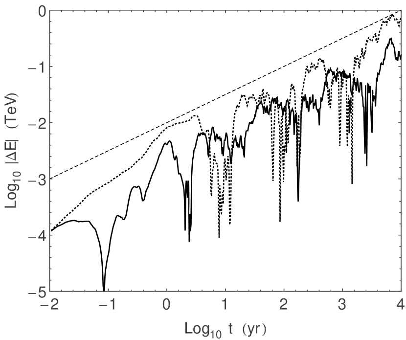
Figure 1: The magnitude of the change in particle energy $|\Delta E_{p}|$ as a function of time for protons with initial energies of $10^{2}$ TeV (solid curve) and $10^{3}$ TeV (dotted curve) moving through turbulent magnetic and electric fields characterized by $\Gamma=3/2$, $\lambda_{\rm max}=1$ pc, $\lambda_{\rm min}=10^{-4}$ pc, and $v_{A}=1$ km s^-1. The turbulent magnetic field has an energy density equal to that of a uniform 10 $\mu$G field. The dashed line represents the value of the upper limit $|\Delta E_{p;\;{\rm max}}|$ given by the expression in equation (16).

To simplify the analysis, we define a dimensionless time $\tau=t/t_{0}$, where $t_{0}$ is the inverse of the gyration frequency multiplied by the Lorentz factor for a particle with charge $q=Ze$ and mass $m=Am_{H}$ in a reference field $B_{0}$, as given by the expression

$$t_{0}={\gamma\over\Omega_{0}}=\qquad\qquad\qquad\qquad$$

$$3.5\times 10^{-4}\,{\rm yrs}\,\left({E_{p}\over 1\,{\rm TeV}}\right)\left({A\over Z}\right)\left({B_{0}\over 10\,\mu{\rm G}}\right)^{-1}\;.$$ (21)

We also define a corresponding dimensionless radius vector ${\bf\bar{r}}={\bf r}/R_{g}$. Since we ignore the electric field $\delta E$, $|{\bf u}|=\gamma v/c$ is a constant of the motion. Thus, for relativistic particles ($v\approx c$), setting the value of $R_{g}$ also sets the value of $t_{0}$ (and vice versa) since $R_{g}=ct_{0}$.

Ignoring the electric field, the equations of motion for highly relativistic particles can then be written in dimensionless form as

$${d\hat{\bf u}\over d\tau}={\hat{\bf u}\times{\bf\bar{B}}}\;,$$ (22)

and

$${d{\bf\bar{r}}\over d\tau}=\hat{\bf u}\;,$$ (23)

where ${\bf\bar{B}}={\bf B}/B_{0}$ and $\hat{\bf u}={\bf u}/|{\bf u}|$.

5 The Case of a Purely Turbulent Field

In our formalism, the trajectory of a particle moving through a purely turbulent field is fully described by the four dimensionless parameters $\Gamma$, $u_{A}=v_{A}/c$, $\bar{\lambda}_{\rm min}=\lambda_{\rm min}/R_{g}$ and $\bar{\lambda}_{\rm max}=\lambda_{\rm max}/R_{g}$ (related to the rigidity $\rho$ through the expression $\bar{\lambda}_{{\rm max}}=2\pi/\rho$), along with the adopted prescription for setting the $N$ values of wavevectors $k_{n}$ discussed below Equation (9). It is important to note that as the particle moves through the field, the radius of gyration changes depending on the field strength being sampled. Within this context, $B_{0}$ is taken to be the field strength of a uniform field whose energy density equals that of the turbulent field. In turn, the value of $R_{g}$ represents a characteristic value for a particle’s radius of gyration.

We begin our analysis by considering how motion through a time-dependent turbulent field differs from that of a static turbulent field ($v_{A}=0$). To this end, we calculate the trajectory of a particle over a time $\tau_{max}=10^{5}\,\bar{\lambda}_{\rm max}$ for the case $\Gamma=3/2$ and the following four sets of wavelength ranges $[\bar{\lambda}_{\rm min},\bar{\lambda}_{\rm max}]$: [3,300]; [0.3,30]; [0.03,3]; and [0.003,0.3]. We plot the displacement $\bar{r}$ of each particle as a function of (the dimensionless) time $\tau$ in Figure 2 for the case of a static field ($v_{A}=0$), and in Figure 3 for the case of a time-dependent magnetic field with an adopted fiducial value $v_{A}$ = 1 km s^-1. The long-dashed lines serve as a reference and have slopes of 1/2.

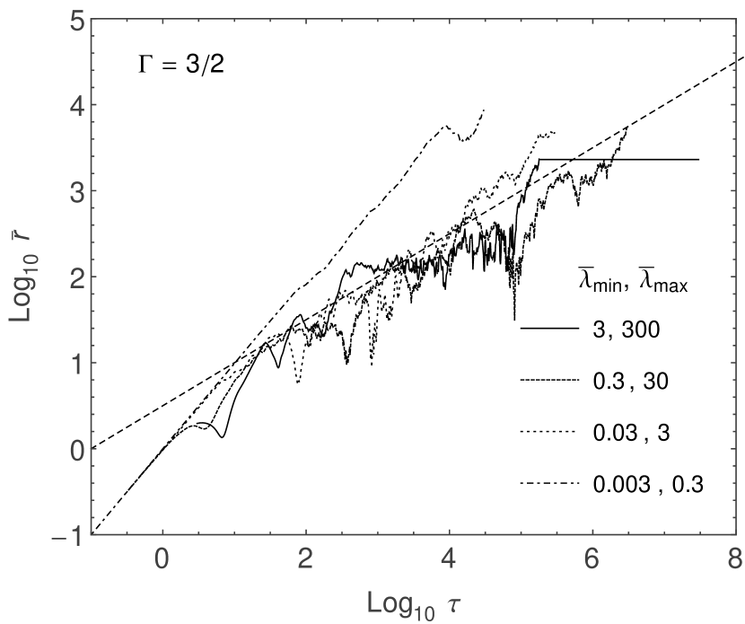
Figure 2: The displacement $\bar{r}$ as a function of time $\tau$ for four particles moving through a static ($v_{A}=0$) turbulent magnetic field with index $\Gamma=3/2$. The values of $\bar{\lambda}_{\rm min}$ and $\bar{\lambda}_{\rm max}$ correspond to the following curves: 3, 300 (solid); 0.3, 30 (short-dashed); 0.03, 3 (dotted); 0.003, 0.3 (dot-dashed). The long-dashed line serves as a reference and has a slope of 1/2.

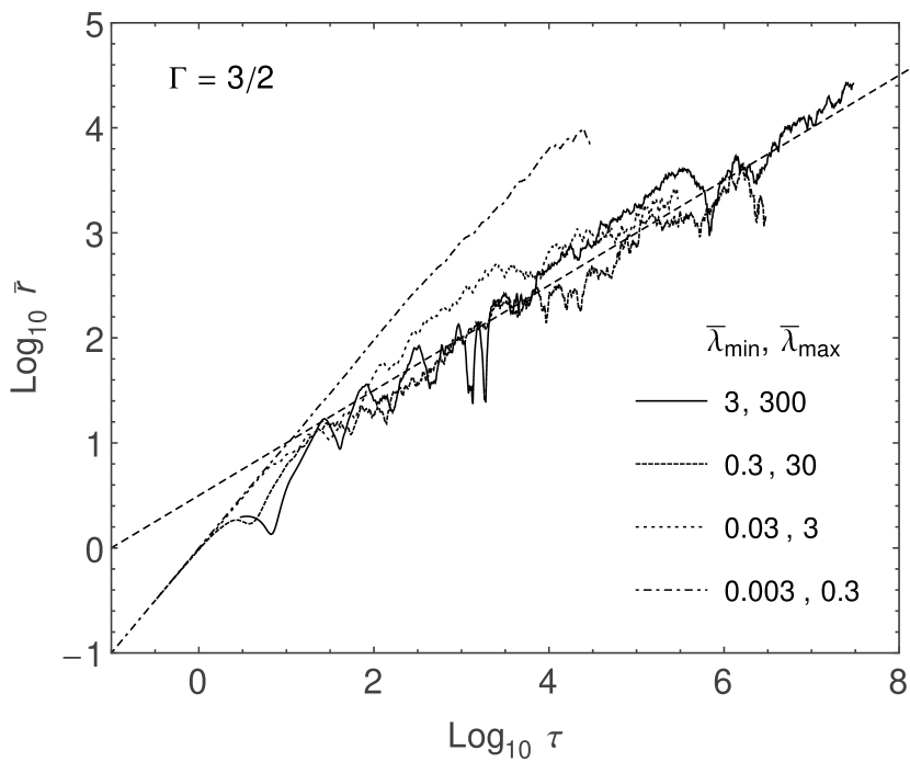
Figure 3: The displacement $\bar{r}$ as a function of time $\tau$ for four particles moving through a temporally fluctuating ($v_{A}=1$ km s^-1) turbulent magnetic field with index $\Gamma=3/2$. The values of $\bar{\lambda}_{\rm min}$ and $\bar{\lambda}_{\rm max}$ correspond to the following curves: 3, 300 (solid); 0.3, 30 (short-dashed); 0.03, 3 (dotted); 0.003, 0.3 (dot-dashed). The long-dashed line serves as a reference and has a slope of 1/2.

Figures 2 and 3 illustrate three important points. First, particles with a radius of gyration below the range of turbulent wavelengths may eventually get trapped in a static field, as can be seen by the fact that $\bar{r}$ is constant at times $\tau>10^{5}$ for the $\bar{\lambda}_{min}=3$ particle (solid line in Figure 2). To gain insight into this phenomenon, we plot in Figure 4 the dot product $\hat{\bf B}\cdot\hat{\bf v}$ as a function of time for the trapped particle shown in Figure 2 (solid curve). One sees that trapping occurs when particles move nearly perpendicular to the local magnetic field, oscillating in a sort of local magnetic bottle. As can be seen in Figure 3 from the solid line at times $\tau>10^{5}$, time-dependent fluctuations will disrupt this trapping on an expected timescale $\tau_{MHD}\sim\bar{\lambda}_{\rm min}/u_{A}$ ($\sim 10^{6}$ for the solid curve shown in Figure 3). Second, once particles with radii of gyration smaller than $\lambda_{\rm max}$ have moved beyond a (dimensionless) distance $\sim\bar{\lambda}_{\rm max}$, their displacement scales as $\bar{r}\propto\tau^{1/2}$. Finally, particles with a radius of gyration greater than the maximum turbulent wavelength are not strongly affected by local turbulence. The motion of such (highly-energetic) particles will not be considered in our analysis.

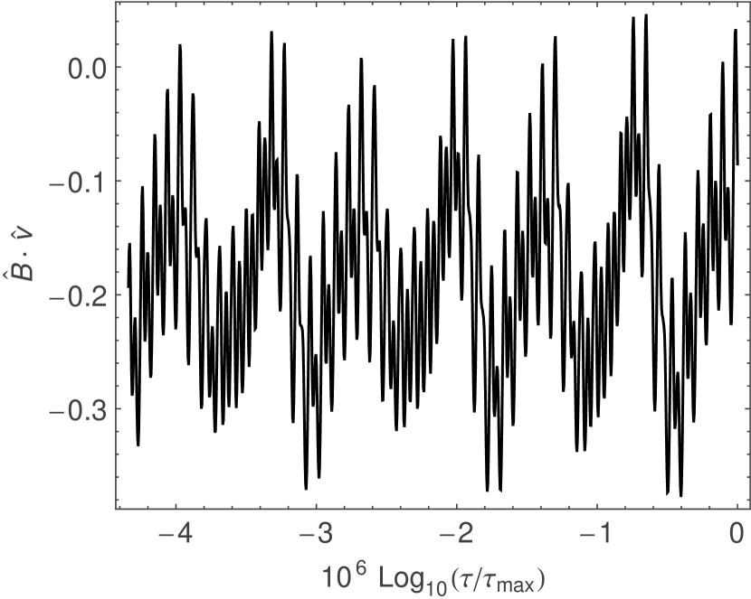
Figure 4: The dot product between the field direction and particle direction of motion as a function of $\tau$ for the trapped particle shown in Figure 2 (solid curve).

The motion of charged particles through a turbulent magnetic field is chaotic in nature. As such, a complete analysis requires a statistical approach. We have therefore performed a suite of experiments designed to adequately sample our parameter space. Specifically, each experiment is defined by a choice of the parameters $\Gamma$, $\bar{\lambda}_{\rm min}$, and $\bar{\lambda}_{\rm max}$. We adopt the value of $v_{A}$ = 1 km s^-1, although in the absence of particle trapping, our results will not be sensitive to this chosen value. For each run, we calculate the trajectory of $N_{p}$ particles injected randomly from the origin for a time $\tau_{max}$, with each particle sampling its own unique magnetic field structure (i.e., the values of $\alpha_{n}$, $\beta_{n}$, $\theta_{n}$, $\phi_{n}$ and the choice of a $\pm$ are chosen randomly for each particle). The suite of experiments performed for the case of a purely turbulent field are summarized in Table 1.

We plot the distributions of $\bar{x}=x/R_{g}$ and $\bar{r}=r/R_{g}$ at time $\tau=10^{3}\,\bar{\lambda}_{\rm max}$ for experiment 2 in Figures 5–6. (The corresponding distributions for experiments 1 and 3 are qualitatively very similar.) Since the particles at this time have fully sampled the turbulent structure of the field, the distributions of their positions $\bar{x}$, $\bar{y}$ and $\bar{z}$ are expected to be normal. For a purely turbulent field, all three distributions are expected to have mean values of zero and equal variances (within the expected statistical fluctuations). Furthermore, since motion along any axis is independent of the others, then the displacement vector $\bar{r}=\sqrt{\bar{x}^{2}+\bar{y}^{2}+\bar{z}^{2}}$ has three independent orthogonal components, each of which follow a standard normal distribution. As such, the $\bar{r}$ values should be distributed according to a chi distribution with 3 degrees of freedom. To illustrate these points, we include the corresponding Gaussian curve derived from the mean and variance in Figure 5, and the corresponding $k=3$ chi distribution in Figure 6. As illustrated by our results, cosmic-ray diffusion through turbulent magnetic fields is well represented by Gaussian statistics.

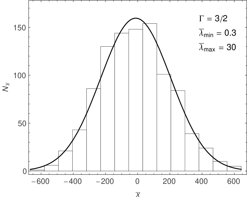
Figure 5: The distribution of $\bar{x}$ values at time $\tau=10^{3}\,\bar{\lambda}_{\rm max}$ for experiment 2 (histogram), superimposed with a Gaussian function (black curve) with the same mean and variance.

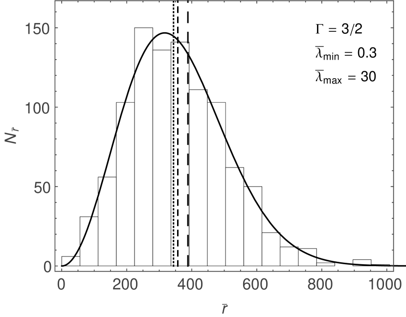
Figure 6: The distribution of $\bar{r}$ values at time $\tau=10^{3}\,\bar{\lambda}_{\rm max}$ for experiment 2 (histogram), superimposed with a chi function of degree 3 (black curve) and scaled using the mean of the $x$, $y$ and $z$ distribution variances. The vertical dotted, short-dashed, and long-dashed lines represent the median, mean and rms values for the distributions, respectively.

The median, mean and rms values of the $\bar{r}$ distribution shown in Figure 6 are denoted, respectively, by the vertical dotted, short-dashed, and long-dashed lines. Although each of these output measures characterize the distribution, we will adopt the mean value $\langle\bar{r}\rangle$ of the particle displacements as our primary output measure, and calculate its value at several times $\tau$ for each experiment performed (as listed in Table 1). In order to determine how sensitive the value of our output measure is on $\bar{\lambda}_{\rm min}$, we compare the results of experiments 1–3 with those of experiments 7, 9 and 11 in Figure 7. As clearly illustrated by the overlap between the results from experiments 1 (open triangle) and 7 (solid triangle), 2 (open square) and 9 (solid square), and 3 (open circle) and 11 (closed circle), particle diffusion depends primarily on the maximum turbulence wavelength $\bar{\lambda}_{\rm max}$, and is not sensitive to the minimum turbulence wavelength $\bar{\lambda}_{\rm min}$, so long as the radius of gyration is greater than the minimum turbulence wavelength (see discussion in §7). Our analysis is therefore greatly simplified in that there is only one primary parameter – $\bar{\lambda}_{\rm max}$ – that dictates how particles diffuse through a purely turbulent field with a specified value of $\Gamma$. We also note that the values of $\langle\bar{r}\rangle$ clearly exhibit the $\tau^{1/2}$ dependence associated with a diffusion process (though particles with $R_{g}\sim\lambda_{\rm max}$ have motions intermediary to their counterparts with smaller radii of gyration and the free-streaming motion of their counterparts with greater radii of gyration).

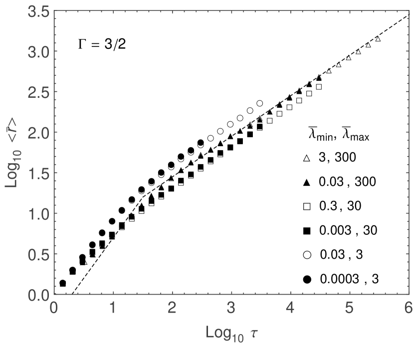
Figure 7: The value of $\langle\bar{r}\rangle$ as a function of $\tau$ for experiments 1 (open triangle), 2 (open square), 3 (open circle), 7 (solid triangle), 9 (solid square) and 11 (solid circle). The dashed lines serve as a reference and have slopes of 1/2 and 1.

We focus the rest of our analysis on cases for which the particle gyration radius falls comfortably within the range of the maximum and minimum turbulence wavelengths so that particles undergo actual diffusion—that is, for which $\bar{\lambda}_{\rm max}\gg 1\gg\bar{\lambda}_{\rm min}$. To do so, we consider a turbulent field with a dynamic range in wavelengths that span either four or five orders of magnitude. We note, however, that the minimal dependence that particle diffusion has on the smallest wavelength implies that our results can be extrapolated to lower values of $\bar{\lambda}_{\rm min}$ (see discussion in §7).

A fundamental issue in this analysis is what value of $N$ will allow our discrete treatment of the turbulent field to adequately represent a continuous field. Toward that end, we first note that the variance of the mean values of $\langle\bar{r}\rangle$ is given by $\sigma_{mean}=\sigma_{\bar{r}}/\sqrt{N_{p}}$. Based on the results presented in Figure 6, $\sigma_{\bar{r}}\sim\langle\bar{r}\rangle/2$, so that the calculated mean of our sample population with $N_{p}=200$ is expected to be within $3\sigma_{mean}=1.5\langle\bar{r}\rangle/\sqrt{N_{p}}\approx 0.1\langle\bar{r}\rangle$ of the true (parent) value with $\sim 99$% confidence. We next perform experiments 6, 16 and 25 with values of $N$ = 50, 100, 200 and 300. The resulting values of $\langle\bar{r}\rangle$ at time $\tau_{max}$ as a function of $N$ are shown in Figure 8, where the error bars represent the expected $3\sigma$ statistical error of $0.1\langle\bar{r}\rangle$. These results appear to justify our adoption of $N=25\,\log_{10}$[$\lambda_{\rm max}/\lambda_{\rm min}$] presented in §2.

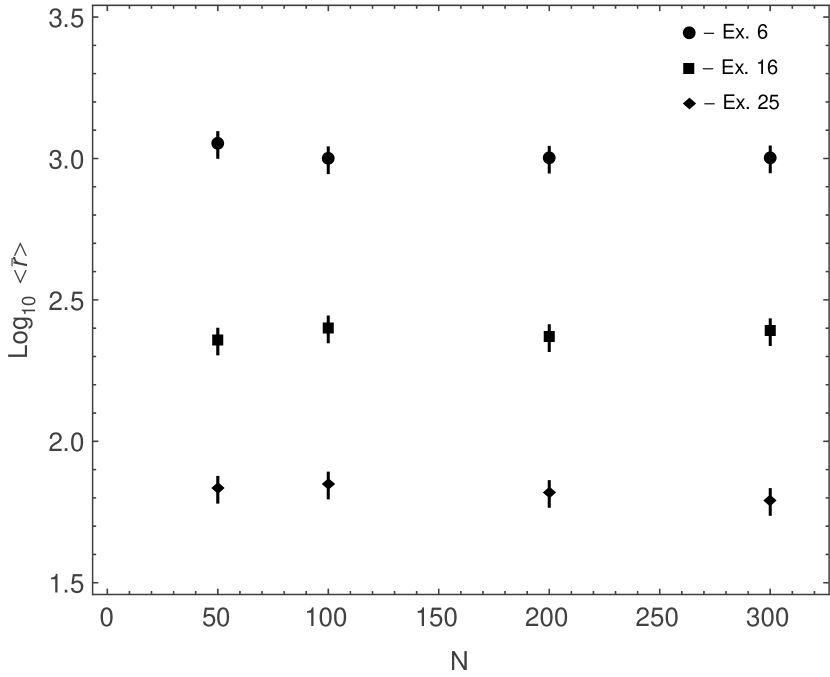
Figure 8: The value of $\langle\bar{r}\rangle$ at $\tau_{max}$ as a function of $N$ for experiments 6, 16, and 25. The error bars represent the expected $3\sigma$ statistical error of 10%.

The results of experiments 4–10, 12–18 and 19–25 are presented in Figures 9, 10 and 11, respectively. A self-similar pattern is clearly visible in these figures for cases with $\bar{\lambda}_{\rm max}\gtrsim 30$, with a break in the slope of the curves from $\sim 1$ to $1/2$ occurring around $\tau\sim\bar{\lambda}_{\rm max}/10$ for $\Gamma=3/2$ and $5/3$, and at $\tau\sim 10$ for $\Gamma=1$. We note, however, that the break is not smooth for the solid circles show in Figures 9, 11 and 12. These irregularities occur as particles with small radii or gyration make transitions from weakly perturbed propagation (for which $\langle\bar{r}\rangle\propto\tau$) to diffusion (for which $\langle\bar{r}\rangle\propto\tau^{1/2}$). This feature indicates that as particles with small radii of gyration make this transition after traveling a distance $\sim 0.1\lambda_{max}$, they are effectively “scattered” randomly in all directions, so that on average, their distance from the origin does not change appreciably until they truly reach the diffusion regime (i.e. they have been “scattered” numerous times).

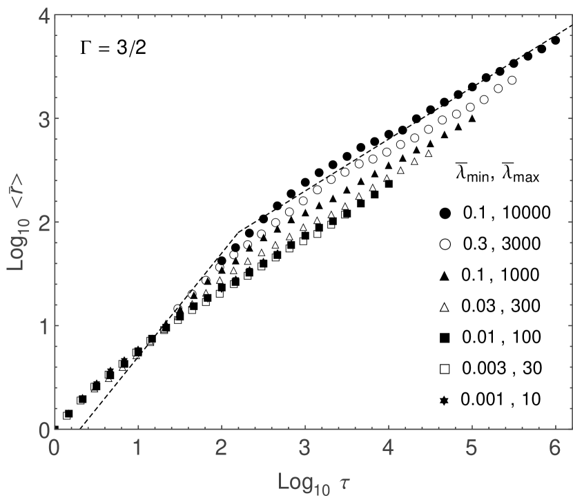
Figure 9: The value of $\langle\bar{r}\rangle$ as a function of $\tau$ for experiments 4–10, for which $\Gamma=3/2$. The dashed lines serve as a reference and have slopes of 1/2 and 1.

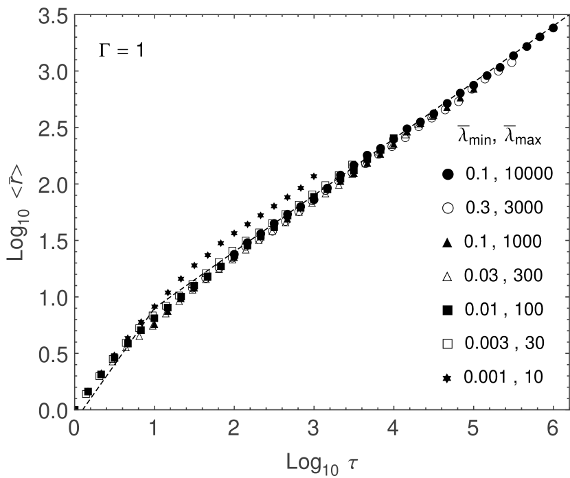
Figure 10: The value of $\langle\bar{r}\rangle$ as a function of $\tau$ for experiments 12–18, for which $\Gamma=1$. The dashed lines serve as a reference and have slopes of 1/2 and 1.

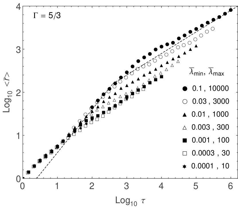
Figure 11: The value of $\langle\bar{r}\rangle$ as a function of $\tau$ for experiments 19–25, for which $\Gamma=5/3$. The dashed lines serve as a reference and have slopes of 1/2 and 1.

In order to put our results into a physical context, we consider relativistic protons moving through a purely turbulent magnetic field for which $\lambda_{\rm max}=1$ pc, and dimensionalize the results of experiments 4–10 accordingly through a proper choice of $R_{g}=\lambda_{\rm max}/\bar{\lambda}_{\rm max}$. We note that setting a common value of $\lambda_{\rm max}$ for experiments 4–25 also sets a common value of $t_{max}=\tau_{max}\,t_{0}=10^{2}\lambda_{\rm max}/c$. The results are presented in Figure 12. As previously noted, the solutions are nearly self-similar for particles whose radius of gyration is $R_{g}\lesssim 0.03\lambda_{\rm max}$.

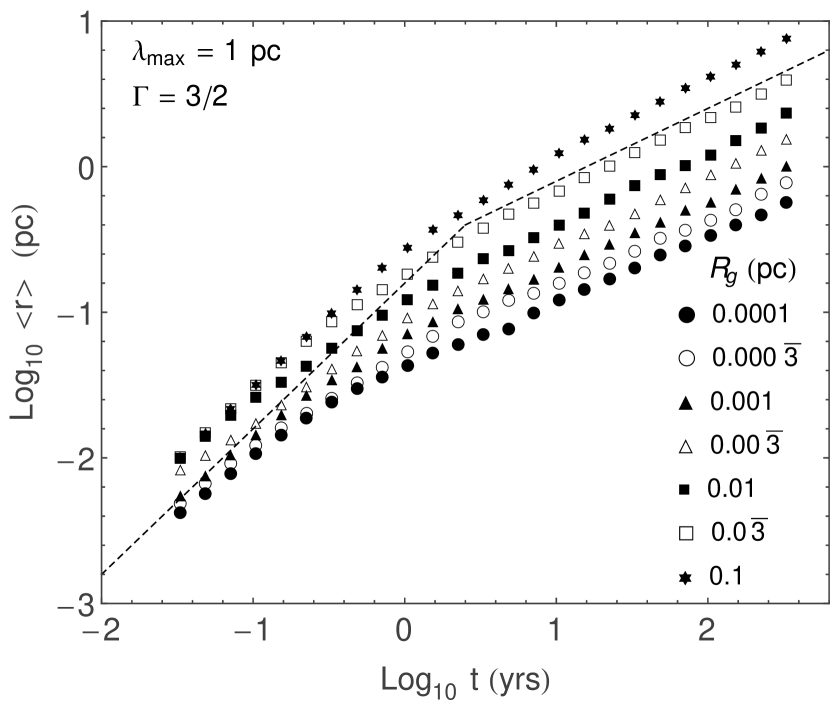
Figure 12: The value of $\langle r\rangle$ as a function of time for experiments 4–10, for which $\Gamma=3/2$. The results of these experiments are dimensionalized by assuming that $\lambda_{\rm max}=1$ pc for each case, and setting the value of $R_{g}$ accordingly. The dashed lines serve as a reference and have slopes of 1/2 and 1.

To better understand how a particle’s gyration radius helps determine the nature of its motion, we plot in Figure 13 particle trajectories of three particles with different radii of gyration, each injected with identical velocity from the origin into the same turbulent (but static) magnetic field defined by $\Gamma=3/2$, $\lambda_{\rm max}=1$ pc, $\lambda_{\rm min}=10^{-4}$ pc, and $B_{0}=10$ $\mu$G. The field line that passes through the origin is depicted by the thin black line. Particle trajectories are depicted by the blue ($R_{g}=0.001$ pc), green ($R_{g}=0.01$ pc) and red ($R_{g}=0.1$ pc) curves. Clearly, the nature of particle motion differs for particles with $R_{g}\lesssim 0.01\lambda_{\rm max}$ and $R_{g}\gtrsim 0.01\lambda_{\rm max}$. For the former, particles are strongly coupled to field lines and their motion is directly tied to the field line structure, whereas for the latter, particles “random walk” through the field. That is not to say that particles with small radii of gyration move smoothly along field lines. Rather, although they are scattered by the turbulent magnetic fields according to their energies, their spread due to scatter is small compared to how far they propagate in the direction of the field.

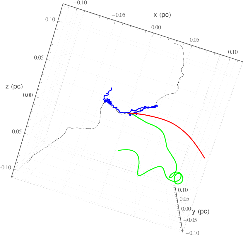
Figure 13: Trajectories of three particles injected with identical velocities from the origin into the same turbulent (but static) magnetic field, defined by $\Gamma=3/2$, $\lambda_{\rm max}=1$ pc, and $\lambda_{\rm min}=10^{-4}$ pc. The colored curves denote the path of particles with gyration radii $0.001$ pc (blue), $0.01$ pc (green), and $0.1$ pc (red). The black curve denotes the magnetic field line passing through the origin.

A central aspect of this work is a determination of the relation between particle diffusion and energy. To that end, we define a dimensionless energy $\epsilon=E_{p}/E_{0}$, where

$$E_{0}=\lambda_{\rm max}\,e\,B_{0}=\qquad\qquad\qquad$$

$$9.2\times 10^{3}\,{\rm TeV}\,\left({\lambda_{\rm max}\over 1\,{\rm pc}}\right)\left({B_{0}\over 10\,\mu{\rm G}}\right)\,,$$ (24)

which then yields the relation $\epsilon=Z\,R_{g}/\lambda_{\rm max}=Z\,\bar{\lambda}_{\rm max}^{-1}$. We plot the values of $\langle r\rangle/\lambda_{\rm max}$ at $\tau_{max}$ as a function of $\epsilon$ in Figure 14 for experiments 4–10, 12–18, and 19–25. Each set of results for a given value of $\Gamma$ demonstrates a clear break at $\epsilon_{b}\sim 0.005$, corresponding to particles with gyration radii $R_{g}\sim 0.005\lambda_{\rm max}/Z$. There is clearly a stronger dependence between $\langle r\rangle$ and $\epsilon$ above the break, presumably due to the fact that particles with $\epsilon<<\epsilon_{b}$ are strongly coupled to the field lines, as shown in Figure 13. As such, their diffusion is dictated primarily by the field structure, and hence, becomes less sensitive to their energy/radius of gyration. Specifically, particles with radii of gyration smaller than $\sim 0.005\lambda_{max}$ will effectively scatter off field fluctuations that have a similar length scale as their gyration radius. In contrast, particles with sufficiently large gyration radii effectively decouple from the field-lines (as is illustrated in Figure 13), and essentially random walk through the field on length scales equal to their gyration radius. Their motion, therefore, is not very sensitive to the nature of the small-scale fluctuations, as can be seen by the convergence of the output values in this regime for the $\Gamma=5/3$ and $\Gamma=1/2$ cases.

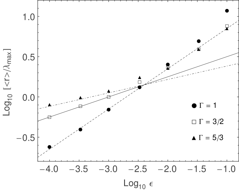
Figure 14: The value of $\langle r\rangle/\lambda_{\rm max}$ evaluated at $\tau_{max}$ as a function of $\epsilon$ for experiments 4–10 ($\Gamma=3/2$), 12–18 ($\Gamma=1$), and 19–25 ($\Gamma=5/3$). The dot-dashed ($\Gamma=5/3$), solid ($\Gamma=3/2$) and dashed ($\Gamma=1$) curves represent power-law fits to the data, as discussed in the text.

In order to put our results into a useful format, we note that in the standard theory for particle diffusion, the turbulent field index $\Gamma$ is related to the diffusion coefficient index $\delta$ (as defined in Equation 2) through the expression $\delta=2-\Gamma$. As such, the diffusion radius $R_{\rm diff}\propto E_{p}^{1-\Gamma/2}\,t^{1/2}$. In turn, we express the particle diffusion length as a function of energy and time through the expression

$${\langle r\rangle}=\lambda_{\rm max}\,\Lambda\left({E_{p}\over E_{0}}\right)^{\alpha}\,\left({t\over t_{c}}\right)^{1/2}\,,$$ (25)

where

$$t_{c}={\lambda_{\rm max}\over c}=3.3\,{\rm yrs}\left({\lambda_{\rm max}\over 1\,{\rm pc}}\right)\,.$$ (26)

We then fit the three lowest-energy data points for each case shown in Figure 14 at time $t=100\,t_{c}$, as illustrated by the dashed ($\Gamma=1$), solid ($\Gamma=3/2$) and dash-dotted ($\Gamma=5/3$) lines, where the corresponding values of $\Lambda$ and $\alpha$ are given in Table 3 for each value of $\Gamma$. In all cases, good fits are obtained with $\alpha=1-\Gamma/2$ for $\epsilon\lesssim 0.005$.

6 Uniform Field with a Turbulent Component

We next consider a molecular cloud environment threaded by a uniform magnetic field with a strong turbulent component. Specifically, we assume a magnetic field of the form ${\bf B}({\bf r},t)=B_{0}\hat{z}+\delta{\bf B}({\bf r},t)$. In our formalism, the motion of a particle moving through such a field is then described by five dimensionless parameters: $\Gamma$, $u_{A}$, $\bar{\lambda}_{\rm min}$, $\bar{\lambda}_{\rm max}$ and $\eta$.

Observations of molecular clouds suggest that the magnetic fluctuations have amplitudes $\delta B\sim B_{0}$. This finding follows from considering the observed non-thermal line-widths in molecular clouds (Larson 1981; Myers et al 1991) to result from MHD waves (e.g., Fatuzzo & Adams 1993; McKee & Zweibel 1995; see Fatuzzo & Adams 2002 for further discussion). We therefore consider the case that the magnetic energy density of the turbulent field equals that of the underlying field, thereby setting $\xi=2$ for all cases explored. The suite of experiments performed are summarized in Table 2.

The introduction of the field $B_{0}\hat{z}$ has broken the isotropy, so we now plot both the distribution of $\bar{x}=x/R_{g}$ and that of $\bar{z}=z/R_{g}$ at time $\tau=10^{2}\,\bar{\lambda}_{\rm max}$ for experiment 5 (Table 2) in Figures 15 and 16, were the solid curves depict the corresponding Gaussians derived from the mean and variance of each distribution. As illustrated by our results, cosmic-ray diffusion through uniform magnetic fields with strong turbulent components is fairly well represented by Gaussian statistics.

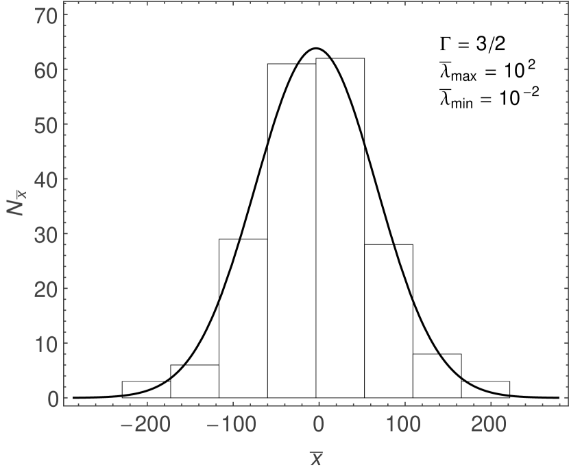
Figure 15: The distribution of $\bar{x}$ values at time $\tau=10^{2}\bar{\lambda}_{\rm max}$ for experiment 5 in Table 2 (histogram), superimposed with a Gaussian function (black curve) with the same mean and variance.

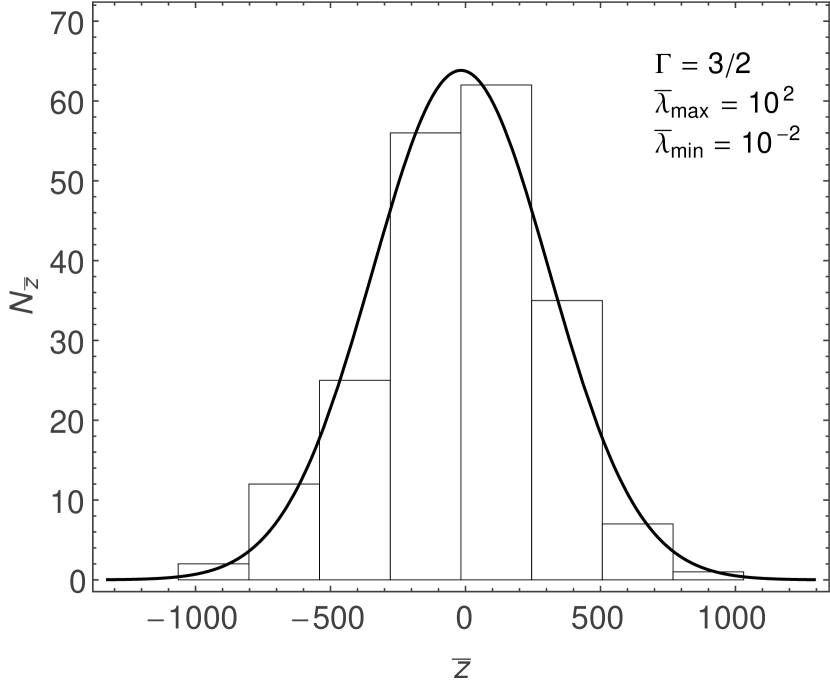
Figure 16: The distribution of $\bar{z}$ values at time $\tau=10^{2}\bar{\lambda}_{\rm max}$ for experiment 5 in Table 2 (histogram), superimposed with a Gaussian function (black curve) with the same mean and variance.

The rms values of the particle positions $\bar{x}$ and $\bar{z}$ at several times $\tau$ for each experiment are shown in Figures 17 and 18. As found for the purely turbulent field discussed in §5, the curves appear to be nearly self-similar, with a break in the slope of the curves occurring at around $\tau\sim\bar{\lambda}_{\rm max}/10$. Not surprisingly, particles diffuse further along the direction of the uniform field than they do across the field, with $\bar{z}_{rms}\sim 5\bar{x}_{rms}$.

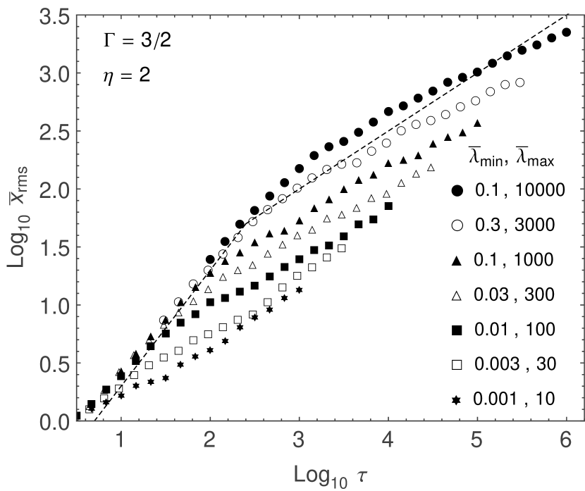
Figure 17: The value of $\bar{x}_{rms}$ as a function of $\tau$ for experiments 1–7 listed in Table 2. The dashed lines serve as a reference and have slopes of 1/2 and 1.

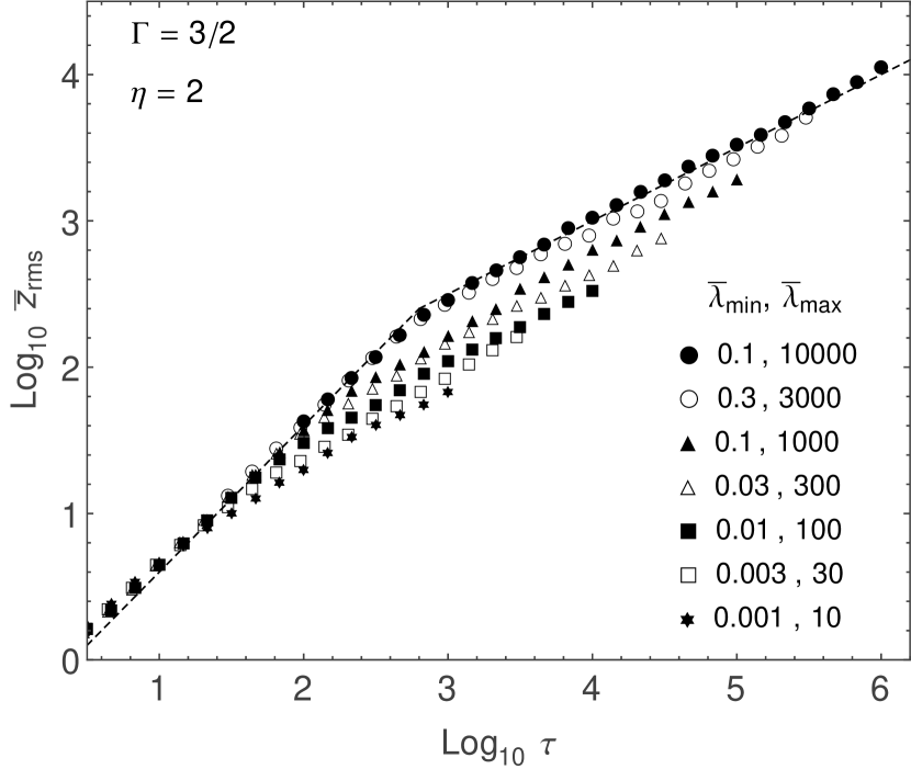
Figure 18: The value of $\bar{z}_{rms}$ as a function of $\tau$ for experiments 1–7 listed in Table 2. The dashed lines serve as a reference and have slopes of 1/2 and 1.

As noted in §5, a central aspect of this work is a determination of the relation between particle diffusion and energy. To that end, we plot the values of $x_{rms}/\lambda_{\rm max}$ and $z_{rms}/\lambda_{\rm max}$ at $\tau_{max}$ as a function of $\epsilon$ in Figure 19 for experiments 1–21 listed in Table 2. In all cases, the data for diffusion along the underlying magnetic field direction is well-fit by a line. Likewise, the data for the diffusion across the underlying magnetic field is well-fit by a line for $\Gamma=1$ and $\Gamma=3/2$, but does exhibit a break at $\epsilon\sim 0.01$ for $\Gamma=5/3$.

Following the analysis presented in §5, we express the particle diffusion lengths across and along the underlying uniform magnetic field through the expressions

$$x_{rms}=\lambda_{\rm max}\,\Lambda_{x}\left({E_{p}\over E_{0}}\right)^{\alpha_{x}}\,\left({t\over t_{c}}\right)^{1/2}\,,$$ (27)

and

$$z_{rms}=\lambda_{\rm max}\,\Lambda_{z}\left({E_{p}\over E_{0}}\right)^{\alpha_{z}}\,\left({t\over t_{c}}\right)^{1/2}\,.$$ (28)

We fit the data in Figure 19 at time $t=100\,t_{c}$, as illustrated by the dashed ($\Gamma=1$), solid ($\Gamma=3/2$) and dash-dotted ($\Gamma=5/3$) lines, where the corresponding values of $\Lambda$ and $\alpha$ are given in Table 4 for each value of $\Gamma$. In all cases except for $x_{rms}$ when $\Gamma=1$, good fits are obtained with $\alpha=1-\Gamma/2$ for the entire range of $\epsilon$ explored.

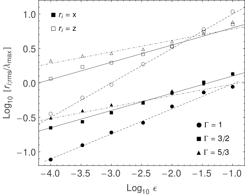
Figure 19: The values of $x_{rms}/\lambda_{\rm max}$ (solid) and $z_{rms}/\lambda_{\rm max}$ (open) evaluated at $\tau_{max}$ as a function of $\epsilon$ for experiments 1–7 ($\Gamma=3/2$), 8–14 ($\Gamma=1$), and 15–21 ($\Gamma=5/3$) listed in Table 2. The dot-dashed ($\Gamma=5/3$), solid ($\Gamma=3/2$) and dashed ($\Gamma=1$) curves represent fits to the data, as discussed in the text.

7 Comparison to Previous Work

The transport properties for charged particles moving through turbulent magnetic fields was analyzed by Casse et al. (2002) using a method similar to that adopted in our work. Specifically, these authors performed extensive numerical experiments using the formalism developed by Giacalone & Jokipii (1994) in order to determine the pitch angle, scattering rate, and the parallel and perpendicular spatial diffusion coefficients for a wide range of rigidities and turbulence levels. Both parallel and perpendicular diffusion coefficients are plotted versus rigidity $\rho=R_{g}k_{min}=2\pi/\bar{\lambda}_{max}$ for several different values of turbulence level

$$\eta={\langle{\bf\delta B}^{2}\rangle\over B_{0}^{2}+\langle{\bf\delta B}^{2}\rangle}\;.$$ (29)

We note that Casse et al. (2002) employed two different methods to construct their magnetic fields. For $\eta=1$ (which represents a purely turbulent field), these authors adopted the same scheme presented in our work, and used a dynamic range in wavelengths of $\lambda_{max}/\lambda_{min}=10^{4}$. For all other cases, the magnetic field was constructed using a fast-Fourier transform (FFT) algorithm to set up the magnetic field on a discrete grid in configuration space. An interpolation scheme was then used to calculate the field at any point in space. For this latter method, $\lambda_{max}/\lambda_{min}=128$ for most cases.

Our analysis extends the work of Casse et al. (2002) in two ways. First, while these authors focused exclusively on Kolmogorov diffusion, we also consider Bohm and Kraichnan diffusion. Second, we extend considerably the dynamic range of turbulence wavelengths, especially for the case of a uniform field with underlying turbulence. In addition, we focus our results to the propagation of cosmic-rays in molecular cloud environments. Nevertheless, sufficient overlap exists for a direct comparison of a subset of our works. Specifically, experiments 19 - 25 listed in Table 1 (purely turbulent field) can be compared directly with the $\eta=1$ data presented in Figure 4 of Casse et al. (2002). In order to do so, we calculate the corresponding diffusion coefficients

$${D\over R_{g}c}={\langle\Delta\bar{x}^{2}\rangle\over 2\tau_{max}}\;,$$ (30)

where $\Delta\bar{x}$ is the particle displacement (from the origin) along the $x$ direction (although all directions are equivalent) evaluated at time $\tau=\tau_{max}$. We note that this method, while not exactly similar, is analogous to that adopted by Casse et al. (2002). As shown in Figure 20, our results (open squares) are in agreement with those of our predecessors (filled circles), with the dotted line denoting the value of $\rho_{min}=2\pi/\bar{\lambda}_{max}$ used in their calculations.

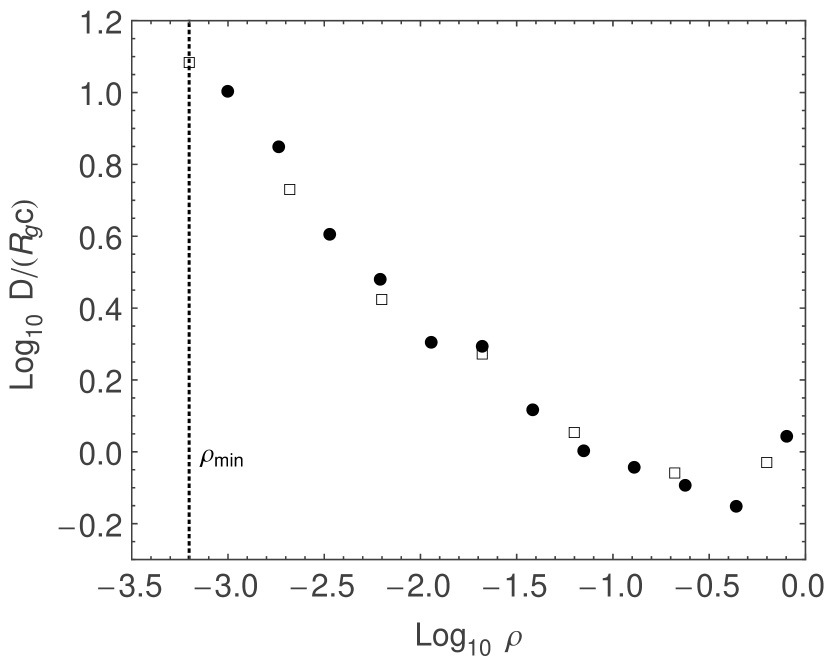
Figure 20: Comparison of the diffusion coefficients calculated for experiments 19 - 25 listed in Table 1 (open squares) with the corresponding diffusion coefficients presented in Figure 4 of Casse et al. 2002 (filled circles). The dotted vertical line denotes the value of $\rho_{min}=2\pi/\bar{\lambda}_{max}$ adopted by this earlier work for the results shown here.

We next compare our results from §6 for the case of a uniform field with underlying turbulence to the $\eta=0.46$ case presented in Figures 4 and 5 of Casse et al. (2002). To do so, we calculate both perpendicular and parallel diffusion coefficients

$${D_{\perp}\over R_{g}c}={\langle\Delta\bar{x}^{2}\rangle\over 2\tau_{max}}\;,\qquad{D_{||}\over R_{g}c}={\langle\Delta\bar{z}^{2}\rangle\over 2\tau_{max}}\;,$$ (31)

for experiments 15 - 21 in Table 2. We compare our results (open squares and circles) to those of our predecessors (filled squares and circles) in Figure 21. The dotted line denotes the value of $\rho_{min}=2\pi/\bar{\lambda}_{max}$ used by Casse et al. (2002) for this case. As expected, the results are in good agreement for $\rho>\rho_{min}$, but deviate for lower values of rigidity, further illustrating our conclusion from §5 that particle diffusion is not sensitive to the value of $\lambda_{min}$ so long as $R_{g}>\lambda_{min}$.

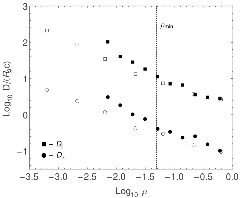
Figure 21: Comparison of the parallel (open squares) and perpendicular (open circles) diffusion coefficients calculated for experiments 15 - 21 listed in Table 2 with the corresponding diffusion coefficients ($\eta=0.46$) presented in Figures 4 and 5 of Casse et al. 2002 (filled squares and circles). The dotted vertical line denotes the value of $\rho_{min}=2\pi/\bar{\lambda}_{max}$ adopted by this earlier work for the results shown here.

8 Application to Cosmic-ray Diffusion in Molecular Clouds

One of the original motivations for this calculation was to determine what kind of injection profile would be required in order to correctly interpret the apparent correlation between the diffuse $\gamma$-ray emissivity and the distribution of molecular gas in the interstellar medium. Such a correlation between $\gamma$-ray intensity maps and the large-scale features of the diffuse gas was first noted in observations ($E_{\gamma}\geq$ 100 MeV) with the SAS-2 and COS B satellite telescopes, combined with radio data that reveal the column density of interstellar hydrogen. Later observations associated at least ten EGRET sources with SNRs expanding into MCs (Esposito et al. 1996; Combi et al. 1998, 2001; Torres et al. 2003). More recently—and more spectacularly—a strong correlation between TeV emission and the molecular gas distribution at the Galactic center was demonstrated by HESS (Aharonian et al. 2006a; Wommer et al. 2008). These data lend support to the idea that the low latitude $\gamma$-ray emission is mainly due to the decay of neutral pions produced by the scattering of cosmic rays with protons in the ambient medium rather than from bremsstrahlung or inverse Compton (IC) scattering.

In their assessment of this effect, Aharonian and Atoyan (1996) argued that the principal region of interest for the $\pi^{0}$-decay $\gamma$-ray emission ought to lie within an $R\leq$ 100 pc region surrounding the cosmic-ray source. Within this distance of a “typical” particle accelerator, a total energy output of $W_{p}\sim 10^{50}$ erg translates into a mean particle energy density of $w_{p}=W_{p}/(4/3)\pi R^{3}\approx 0.55(W_{p}/10^{50}\;{\rm erg})(R/100\;{\rm pc})^{-3}$ eV/cm³, which may significantly exceed the average level of the “sea” of galactic cosmic rays with energy density $w_{0}\approx$ 1 eV/cm³. Therefore, in a 1^∘–10^∘ region around a cosmic-ray source (depending on the distance to the source), we should expect to see higher than average $\gamma$-ray emission. In addition, if the diffusive propagation of cosmic rays is energy-dependent, the resulting $\gamma$-ray spectrum will differ from the $\gamma$-ray spectrum produced by galactic cosmic rays (e.g., Fujita et al. 2009). Thus, the possibility of having several dense giant molecular clouds (GMCs) in close proximity to a particle accelerator will not only produce higher than average levels of $\gamma$-rays but may give the appearance that there are multiple distinct cosmic-ray sources or, due to the limited angular resolution of instruments like EGRET, an extended cosmic-ray source. Accurately predicting the spatial and temporal evolution of the $\gamma$-ray spectrum produced by a particle accelerator may therefore lead to the classification of tens of unidentified EGRET sources.

In order to apply our results from §§5 and 6 to molecular cloud environments, we consider the ideal case of a single impulsive cosmic-ray source surrounded by a homogeneous molecular cloud of radius $R$. While the value of $\lambda_{\rm max}$ is not known for such environments, one would expect its value to be constrained from below by the size of dense cores ($\sim 0.1$ pc) and from above by the size of the actual cloud ($\sim 10-20$ pc). We therefore adopt the intermediary value of $\lambda_{\rm max}=1$ pc in our discussion (although we keep $\lambda_{max}$ in our scaled equations below). The energy range $10^{-4}\leq\epsilon\leq 0.1$ of our work (as shown in Figures 14 and 19) thus corresponds to a true particle energy range of $1\lesssim E_{p}\lesssim 10^{3}$ TeV. In turn, since only $\sim 10\%$ of a relativistic protons’ energy goes into the $\pi_{0}$ photon decay channel for $pp$ scattering (see, e.g., Fatuzzo et al. 2006), the corresponding energy range of $\gamma$-rays resulting from the interaction of these CR’s and the ambient molecular cloud medium is $0.1\lesssim\epsilon_{\gamma}\lesssim 10^{2}$ TeV, which falls within the range observable by HESS.

As shown by Aharonian and Atoyan (1996), the energy loss rate of protons with energies needed to produce $\pi^{0}$-decay $\gamma$-rays is dominated by nuclear energy losses due to $pp$ scattering with the ambient medium. The lifetime of the protons, $\tau_{pp}$, depends on the pp-scattering cross-section, $\sigma_{pp}$, and the inelasticity parameter, $\kappa$. Over a broad range of proton energies, neither of these quantities significantly varies so the usual method is to adopt the constant average values $\sigma_{pp}\approx$ 40 mb and $\kappa\approx$ 0.45 (see, e.g., Markoff et al. 1997). That being the case, the proton lifetime becomes independent of proton energy:

$$\tau_{pp}=(nc\kappa\sigma_{pp})^{-1}\approx 3\times 10^{5}\;{\rm yr}\,\left({n_{H_{2}}\over 100\;{\rm cm}^{-3}}\right)^{-1}\;,$$ (32)

where $n$ is the number density of ambient protons (i.e., $n=2n_{H_{2}}$).

We compare this timescale to the particle escape time $\tau_{e}$, defined here as the time it takes CR’s to diffuse a distance $\langle r\rangle=R$ for purely turbulent fields, and $\langle z_{rms}\rangle=R$ if an underlying uniform field threads the molecular cloud. For the intermediary case of Kraichnan diffusion, Equations 21 – 23 can be combined to yield the expression

$$\tau_{e;{\rm turb}}\approx 4\times 10^{5}\,{\rm yrs}\,\left({R\over 20\,{\rm pc}}\right)^{2}\,\qquad$$

$$\left({E_{p}\over 1\,{\rm TeV}}\right)^{-1/2}\left({\lambda_{\rm max}\over 1\,{\rm pc}}\right)^{-1/2}\,\left({B_{0}\over 10\,\mu{\rm G}}\right)^{1/2}\,.$$ (33)

Likewise, Equations 21, 23 and 25 can be combined to yield the expression

$$\tau_{e;{\rm unif}}\approx 10^{5}\,{\rm yrs}\,\left({R\over 20\,{\rm pc}}\right)^{2}\,\qquad$$

$$\left({E_{p}\over 1\,{\rm TeV}}\right)^{-1/2}\left({\lambda_{\rm max}\over 1\,{\rm pc}}\right)^{-1/2}\,\left({B_{0}\over 10\,\mu{\rm G}}\right)^{1/2}\,.$$ (34)

As suggested by Figure 1, injected particles will therefore gain a modest energy of $\sim 1$ TeV due to acceleration from the turbulent electric fields before they escape. As such, the fits to the data presented in Figures 14 and 19 (as summarized by Equations 22 – 25) cannot be extrapolated to lower energies for molecular cloud environments (since $\epsilon=10^{-4}$ represents a particle energy of 0.92 TeV under the assumed conditions).

Given the similarity between $\tau_{pp}$ and $\tau_{e}$, a significant fraction of $>$ TeV CR’s will likely undergo $pp$ scattering before escaping from the molecular cloud environment. As this fraction decreases with increasing energy, the resulting $\gamma$-ray spectrum will be softer than that of the injected particle spectrum (e.g., Fujita et al. 2009). In addition, if magnetic fields in molecular clouds are purely turbulent, then the break in the $\langle r\rangle$ – $\epsilon$ data shown in Figure 14 at $\epsilon\sim 0.005$ – which for the assumed conditions corresponds to a value of $E_{p}\sim 50$ TeV – would likely produce a break in an observed $\gamma$-ray spectrum at around $\epsilon_{\gamma}\sim 5$ TeV. Such a break would not be observed if molecular clouds are threaded by an underlying uniform magnetic field (see, e.g., Figure 19).

The total $\gamma$-ray luminosity expected from our assumed molecular cloud with a singe injection source $W_{p}$ is independent of the escape time, as can be seen through the simple estimate

$$L_{\gamma}\approx f\left({\tau_{e}\over\tau_{pp}}\right)\,\left({W_{p}\over\tau_{e}}\right)=10^{36}\,{\rm erg}\,{\rm s}^{-1}$$

$$\left({f\over 0.1}\right)\,\left({W_{p}\over 10^{50}\,{\rm erg}}\right)\left({\tau_{pp}\over 3\times 10^{5}{\rm yr}}\right)^{-1}\;,$$ (35)

where $f$ takes into account that only $\sim 10\%$ of the relativistic protons’ energy goes into the $\pi_{0}$ photon decay channel.

Interestingly, this value is in reasonable agreement with the $\approx 10^{35}$ erg s^-1 luminosities in the 0.1 - 100 GeV band inferred for four SNR’s interacting with molecular clouds (G349.7+0.2; CTB 37A; 3C 391; G8.7-0.1) observed by the Large Area Telescope on board the Fermi Gamma-ray Space Telescope (Castro & Slane 2010). Two of these SNRs (CTB 37A and G8.7-0.1) are also possible counterparts to HESS sources with implied luminosities in the 0.2 - 10 TeV band of $\approx 5\times 10^{34}$ ergs s^-1 and $\approx 2\times 10^{35}$ erg s^-1, respectively, and three additional HESS sources coincident with SNRS G338.3-0.0, G12.82-0.02 and W41 have implied 0.2 - 10 TeV luminosities of $\approx 2\times 10^{35}$ erg s^-1, $3\times 10^{34}$ erg s^-1, and $4\times 10^{34}$ erg s^-1, respectively (Aharonian et al. 2006b) . Finally, we note that the above expected luminosity also falls within the range $1\times 10^{34}$–$4\times 10^{36}$ ergs s^-1 inferred from observations of the EGRET SNRs, although the energy range of this instrument only goes up to $\sim 30$ GeV.

9 Conclusion

We have investigated how high-energy CR’s propagate through molecular cloud environments using a modified numerically based formalism developed by Giacalone & Jokipii (1994) for the general study of cosmic-ray diffusion, thereby providing a baseline analysis for two magnetic field configurations: 1) a purely turbulent field; and 2) a uniform magnetic field with a strong turbulent component. We have focused most of our analysis on cases for which the particle gyration radius $R_{g}$ falls comfortably within the range of wavelengths shaping the turbulence. For a purely turbulent field, the trajectory of a particle is fully described by four dimensionless parameters. However, we have found that the diffusion of an ensemble of particles through a turbulent field (characterized by the index $\Gamma$) depends primarily on only one of these—the dimensionless scale length $\bar{\lambda}_{\rm max}\equiv\lambda_{\rm max}/R_{g}$. For a uniform field with a turbulent component, CR diffusion depends on one additional dimensionless parameter—the ratio of turbulent field energy density to the uniform field energy density.

Given the chaotic nature of particle motion through turbulent magnetic fields, we performed a suite of statistical experiments as defined by the dimensionless parameters listed in Table 1 (a purely turbulent field) and Table 2 (a uniform field plus a strong turbulent component). Specifically, we calculated the trajectory of $N_{p}$ particles injected randomly from the origin for a time $\tau_{max}$ for each experiment, with each particle sampling its own unique (and randomly selected) magnetic field structure. The resulting distributions of particle displacement along a given axis were found to be well described by Gaussian profiles with the same mean and variance, thereby justifying our use of the mean of the particle displacements $\langle r\rangle$ as our output measure for characterizing the diffusion of particles through purely turbulent fields, and the rms values of the particle positions $x_{rms}$ and $z_{rms}$ as our output measures for a uniform magnetic field $B_{0}\hat{z}$ with a strong turbulent component. We have found that after an initial time during which particles travel a distance $\sim\lambda_{\rm max}$, each of these output measures scales as $\sqrt{t}$, as expected for a diffusion process.

The results of our analysis indicate that particle diffusion behaves differently for gyro radii in the ranges $0.01\lambda_{\rm max}\lesssim R_{g}\lesssim\lambda_{\rm max}$ and $R_{g}\lesssim 0.01\lambda_{\rm max}$. Specifically, we have found that in the former case, particles “random walk” through the field, whereas for the latter, particles are strongly coupled to field lines and their motion is directly tied to the field line structure. In turn, the distance over how far particles diffuse in purely turbulent fields as a function of energy exhibits a clear break at the point where the particle’s gyration radius $R_{g}\approx 0.005\lambda_{\rm max}$.

Comparing our results with those obtained in earlier works, we find good agreement with previous results obtained using the same formalism (e.g., Casse et al. 2002). In addition, our results are well-fit by the “standard” scaling law $R_{\rm diff}\propto E_{p}^{1-\Gamma/2}$ often invoked in the literature. We provide simple scaling relations between mean diffusion lengths and energy for both magnetic field profiles considered. We note, however, that these scaling-laws lead to a significant underestimation of the diffusion lengths for the case of purely turbulent fields at energies $E_{p}\gtrsim 0.005\,\lambda_{max}\,e\,B_{0}$. In addition, the index $1-\Gamma/2$ is not valid for the case of Bohm diffusion ($\Gamma=1$) perpendicular to an underlying uniform magnetic field.

The results of our work have important consequences for properly connecting $\gamma$-ray spectra associated with molecular clouds to the underlying particle populations. We find that a significant fraction of $>$ TeV CR’s will likely undergo $pp$ scattering before diffusing out of a molecular cloud environment. As this fraction decreases with increasing energy, the resulting $\gamma$-ray spectrum will be softer than that of the injected particle spectrum (e.g., Fujita et al. 2009). In addition, if magnetic fields in molecular clouds are purely turbulent, then the break in the $\langle r\rangle$ – $\epsilon$ dependence (as shown in Figure 14) is expected to produce a corresponding break in an observed $\gamma$-ray spectrum at around $\epsilon_{\gamma}\sim 5$ TeV. Such a break would not be observed if molecular clouds are threaded by an underlying uniform magnetic field.

The work we have reported here has consequences for other types of high-energy sources as well. For example, the compact object 1E 1740, embedded within a molecular cloud at the galactic center, produces a jet of (presumably) relativistic electrons and positrons (Misra & Melia 1993) that eventually diffuse into the surrounding medium. The diffuse radio inensity from this region provides some measure of the lepton injection rate, but it clearly also depends on the energy-dependent diffusion rate through the molecular gas. The results reported here for proton diffusion cannot be directly generalized to the case of positrons, but we anticipate seeing qualitative similarities between the two once we have completed the analogous positron simulations.

The galactic center hosts a complex array of diffuse emitters, in addition to the TeV sources we have discussed in this paper. A proper analysis of the underlying nonthermal particle population producing this emission should therefore include observations at $\gamma$-ray (and even hard X-ray) energies, in addition to the HESS data we have considered here (see, e.g., Belanger et al. 2004; Rockefeller et al. 2004). In future work, we will more closely examine the observational consequences of the different behavior of CR’s above and below the break energy $E_{b}$, particularly as it impacts the diffuse broadband emission within $\sim$20 pcs of the supermassive black hole Sgr A*.

Of course, Sgr A* itself is apparently a significant accelerator of relativistic electrons and protons (Liu et al. 2006), the latter diffusing (Ballantyne et al. 2007) through the captured, accreting gas (Ruffert and Melia 1994; Falcke et al. 1997) into the surrounding medium, possibly producing the HESS point source coincident with the black hole. However, attempts at reconciling this TeV emission with the longer wavelength radiation produced closer to the center have been hampered by the uncertain energy-dependence of this diffusion process. As we have discussed in this paper, a detailed knowledge of the diffusion coefficient is essential for meaningfully connecting the observed spectrum to the underlying nonthermal particle population. We will be applying the conclusions reached here to this important problem and will report the results elsewhere.

Table 1: Experiments for A Purely Turbulent Field

Exp	$\Gamma$	$\bar{\lambda}_{\rm min}$	$\bar{\lambda}_{\rm max}$	$N_{p}$	$\tau_{max}/\bar{\lambda}_{\rm max}$
1	3/2	3	300	1000	$10^{3}$
2	3/2	0.3	30	1000	$10^{3}$
3	3/2	0.03	3	1000	$10^{3}$
4	3/2	0.1	10,000	200	$10^{2}$
5	3/2	0.3	3,000	200	$10^{2}$
6	3/2	0.1	1,000	200	$10^{2}$
7	3/2	0.03	300	200	$10^{2}$
8	3/2	0.01	100	200	$10^{2}$
9	3/2	0.003	30	200	$10^{2}$
10	3/2	0.001	10	200	$10^{2}$
11	3/2	0.0003	3	200	$10^{2}$
12	1	0.1	10,000	200	$10^{2}$
13	1	0.3	3,000	200	$10^{2}$
14	1	0.1	1,000	200	$10^{2}$
15	1	0.03	300	200	$10^{2}$
16	1	0.01	100	200	$10^{2}$
17	1	0.003	30	200	$10^{2}$
18	1	0.001	10	200	$10^{2}$
19	5/3	0.1	10,000	200	$10^{2}$
20	5/3	0.3	3,000	200	$10^{2}$
21	5/3	0.1	1,000	200	$10^{2}$
22	5/3	0.03	300	200	$10^{2}$
23	5/3	0.01	100	200	$10^{2}$
24	5/3	0.003	30	200	$10^{2}$
25	5/3	0.001	10	200	$10^{2}$

Table 2: Experiments for A Uniform Field Plus Strong Turbulence

Exp	$\Gamma$	$\eta$	$\bar{\lambda}_{\rm min}$	$\bar{\lambda}_{\rm max}$	$N_{p}$	$\tau_{max}/\bar{\lambda}_{\rm max}$
1	3/2	2	0.1	10,000	200	$10^{2}$
2	3/2	2	0.3	3,000	200	$10^{2}$
3	3/2	2	0.1	1,000	200	$10^{2}$
4	3/2	2	0.03	300	200	$10^{2}$
5	3/2	2	0.01	100	200	$10^{2}$
6	3/2	2	0.003	30	200	$10^{2}$
7	3/2	2	0.001	10	200	$10^{2}$
8	1	2	0.1	10,000	200	$10^{2}$
9	1	2	0.3	3,000	200	$10^{2}$
10	1	2	0.1	1,000	200	$10^{2}$
11	1	2	0.03	300	200	$10^{2}$
12	1	2	0.01	100	200	$10^{2}$
13	1	2	0.003	30	200	$10^{2}$
14	1	2	0.001	10	200	$10^{2}$
15	5/3	2	0.1	10,000	200	$10^{2}$
16	5/3	2	0.3	3,000	200	$10^{2}$
17	5/3	2	0.1	1,000	200	$10^{2}$
18	5/3	2	0.03	300	200	$10^{2}$
19	5/3	2	0.01	100	200	$10^{2}$
20	5/3	2	0.003	30	200	$10^{2}$
21	5/3	2	0.001	10	200	$10^{2}$

Table 3: Fitting parameters for Figure 14

$\Gamma$		$\Lambda$	$\alpha$
1		2.2	0.5
3/2		0.56	0.25
5/3		0.35	0.17

Table 4: Fitting parameters for Figure 19

$\Gamma$		$\Lambda_{x}$	$\alpha_{x}$		$\Lambda_{z}$	$\alpha_{z}$
$1$		0.22	0.36		3.2	0.5
$3/2$		0.22	0.25		1.1	0.25
$5/3$		0.14	0.17		0.89	0.17

References

- aharonian (96) Aharonian, F. A., & Atoyan, A. M. 1996, A&A, 309, 917
- aharonian (06) Aharonian, F., et al. 2006a, Nature, 439, 695
- (3) Aharonian, F., et al. 2006b, ApJ, 636, 777
- ball (07) Ballantyne, D. R., Melia, F., Liu, S., Crocker, R. 2007, ApJL, 657, L13
- bas (00) Basu, S. 2000, ApJL, 540, L103
- belanger (04) Belanger, G. et al. 2004, ApJL, 601, L163
- casetal (02) Casse, F., Lemoine, M., & Pelletier, G. 2002, PhRvD, 65, 023002
- cassla (10) Castro, D., Slane, P. 2010, ApJ, 717, 372
- com (1) Combi, J. A., Romero, G. E., Benaglia, P. 1998, A&A, 333, L91
- com (2) Combi, J. A., Romero, G. E., Benaglia, P., & Jonas, J. L. 2001, A&A, 366, 1047
- cru (99) Crutcher, R. M. 1999, ApJ, 520, 706
- dem (07) De Marco, D., Blasi, P., & Todor, S. 2007. JCAP, 6, 27
- (13) Dorfi, E. A., 1991, A&A, 251, 597
- dorf (2) Dorfi, E. A., 2000, ApSS, 272, 227
- (15) Esposito, J. A., Hunter, S. D., Kanback, G., & Streekumar, P. 1996, ApJ, 461, 820
- fal (97) Falcke, H. and Melia, F. 1997, ApJ, 479, 740
- fat (93) Fatuzzo, M., & Adams, F. C. 1993, ApJ, 412, 146
- fat (02) Fatuzzo, M., & Adams, F. C. 2002, ApJ, 570, 210
- fat (05) Fatuzzo, M., & Melia, F. 2005, ApJ, 630, 321
- fat (06) Fatuzzo, M., Adams, F. C., & Melia, F. 2006, ApJ, 653, L49
- framel (08) Fraschetti, F. & Melia, F. 2008, MNRAS, 391, 1100
- Fujita (09) Fujita, Y., Ohira, Y., Tanaka, S. J., & Takahara, F. 2009, ApJL, 707, L179
- gabici (09) Gabici, S., Aharonian, F. A., & Casanova, S. 2009, MNRAS, 396, 1629
- giajok (94) Giacalone, J. & Jokipii, J. R. 1994, ApJL, 430, L137
- jok (66) Jokipii, J. R. 1966, ApJ, 146, 480
- kowmel (99) Kowalenko, V. & Melia, F. 1999, MNRAS, 310, 1053
- (27) Kulsrud, R., & Pearce, W. P. 1969, ApJ, 156, 445
- ladetal (91) Lada, E. A., Bally, J., & Stark, A. A. 1991, ApJ, 368, 432
- lar (81) Larson, R. B. 1981, MNRAS, 194, 809
- liu (06) Liu, S., Melia, F., Petrosian, V., and Fatuzzo, M. 2006, ApJ, 647, 1099
- markoff (97) Markoff, S., Melia, F., and Sarcevic, I. 1997, ApJL, 489, L47
- Mckzwe (95) McKee, C. F., & Zweibel, E. G. 1995, ApJ, 440, 686
- misra (93) Misra, R. and Melia, F. 1993, ApJL, 419, 25
- myeetal (91) Myers, P. C., Ladd, E. F., & Fuller, G. A. 1991, ApJ, 372, L95
- (35) Ormes, J. F., Ösel, M. E., Morris, D. J. 1988, ApJ, 334, 722
- rock (04) Rockefeller, G., Fryer, C. L., Melia, F., and Warren, M. S. 2004, ApJ, 604, 662
- ruff (94) Ruffert, M. and Melia F. 1994, AA, 288L, L29
- (38) Torres, D. F., et al. 2003, PhR, 382, 303
- wometal (08) Wommer, E., Melia, F., & Fatuzzo, M. 2008, MNRAS, 387, 987