A general T-matrix approach applied to two-body and three-body problems
in cold atomic gases

Abstract

We propose a systematic T-matrix approach to solve few-body problems with s-wave contact interactions in ultracold atomic gases. The problem is generally reduced to a matrix equation expanded by a set of orthogonal molecular states, describing external center-of-mass motions of pairs of interacting particles; while each matrix element is guaranteed to be finite by a proper renormalization for internal relative motions. This approach is able to incorporate various scattering problems and the calculations of related physical quantities in a single framework, and also provides a physically transparent way to understand the mechanism of resonance scattering. For applications, we study two-body effective scattering in 2D-3D mixed dimensions, where the resonance position and width are determined with high precision from only a few number of matrix elements. We also study three fermions in a (rotating) harmonic trap, where exotic scattering properties in terms of mass ratios and angular momenta are uniquely identified in the framework of T-matrix.

I Introduction

Interacting ultracold atoms have gained a lot of research interests for their interaction strength and dimensionality are highly controllable by making use of Feshbach resonance and external confinementsBloch ; Giorgini . In such dilute atomic gases, the interaction between atoms can be well approximated as contact potential which is characterized by the s-wave scattering lengthBloch ; Giorgini . In this context, the few-body problems play very important roles in studying many-body properties. For instance, solutions of these problems determine effective interactions between atom-atom, atom-dimer and dimer-dimerPetrov1 ; Petrov2 , which are fundamental elements to formulate the many-body effective Hamiltonian; moreover, the consideration of two-body short-range physics leads to a series of exact universal relations for a many-body system, as first proposed by TanTan1 ; Tan2 ; Tan3 and recently verified in experimentJin10 .

Previous studies of few-body systems have revealed many nontrivial effects. One famous example is the Efimov effect for three atomsEfimov ; Braaten06 , depending closely on the short-range interacting parameter apart from single s-wave scattering length. Another typical effect is the two-body induced resonance scattering and induced bound state due to external confinementsBusch98 ; Olshanii1 ; Olshanii2 ; Moritz05 ; Petrov00 ; Petrov01 ; Orso05 ; Buechler10 ; Cui10 ; Kestner07 ; Peano ; Castin ; Nishida_mix ; Lamporesi . Among most of previous studies, the problems were solved in the framework of two-channel modelsKokkelmans02 or by using pseudopotentialsLHY1 ; LHY2 . In this article, we present using T-matrix approach to solve few-body problems with s-wave contact interaction in the field of ultracold atoms. Compared with other methods, T-matrix is able to systematically provide exact solutions for few-body problems, and more importantly, is able to work in a much efficient and physically transparent way.

In this article, we shall first formulate T-matrix method and introduce its essential concept, i.e., the renormalization idea to integrate out all high-energy(or short-range) contributions for relative motions. Then a systematic treatment is presented to a general N-body system with contact interactions and with possibly trapping potentials. The key point of this method is to make use of the interaction property and introduce a set of orthogonal molecular states, which describe the external center-of-mass(CM) motions of pairs of interacting particles; then the problem is generally reduced to a matrix equation, and a proper renormalization scheme for the internal relative motions ensures finite value of each matrix element. Using this method, we obtain the bound state solution, scattering matrix element and reduced coupling constant in the low-dimensional subspace. Moreover, the treatment has a lot more physical meanings and allows us to make analytical predictions to various induced resonances under confinement potentials. In all, T-matrix approach is able to unify many studies of different issues in the single framework.

To show the efficiency of this approach, we apply it to study two-body effective scattering in 2D-3D mixed dimensions, where T-matrix not only provides a transparent way to understand the mechanism of multiple resonances, but also gives explicit expressions for the resonance position and the width. Particularly, its efficiency lies in that each resonance can be determined accurately by only calculating a few number of matrix elements. Moreover, we apply this method to study three two-component fermions in a (rotating) harmonic trap, and show its unique advantage in identifying scattering properties in different angular momentum channels. The ground state is obtained for a rotating and trapped system, which gives important hints for quantum Hall physics in the fermionic atom-dimer system.

The rest of this paper is organized as follows. In section II, we introduce the renormalization concept and present T-matrix formulism to solve a general few-body problem. Its relations to other approaches, advantages and limitations are also discussed. Section III is the application of T-matrix approach to two-body problems, where specifically we study the scattering resonances in 2D-3D mixed dimensions. Section IV is the application to three fermions in a (rotating) harmonic trap, where the energy spectrum and scattering property are studied for different mass ratios and angular momenta of three fermions. We summarize the paper in the last section.

II T-matrix approach

In this section we give a systematic prescription of T-matrix approach to solve few-body problems. The resulted matrix equation is given by Eq.10 in Section IIA, from which we extract three important physical quantities as given by Eqs.(12,14,18) in Section IIB. We also discuss its relation to other widely used methods in Section IIC, and demonstrate its unique advantages and limitations in Section IID.

II.1 Basic concept and general formulism

We start from the Lippmann-Schwinger equation based on standard scattering theory,

$$|\psi\rangle = |\psi_{0}\rangle+\hat{G}_{0}(E)\hat{T}|\psi_{0}\rangle.$$ (1)

Here $|\psi_{0}\rangle$ is the eigen-state for non-interacting system, with Hamiltonian $\hat{H}_{0}=\hat{H}_{{\rm kin}}+\hat{V}_{T}$ composed by kinetic term and external trapping potential; $|\psi\rangle$ is the scattered state in the presence of interaction potential $\hat{U}$;

$$\hat{G}_{0}(E)=\frac{1}{E-\hat{H}_{0}+i\delta}$$ (2)

is the Green function; the scattering matrix can be expanded as series $T=U+UG_{0}U+UG_{0}UG_{0}U+...$ which leads to

$$T = (1-UG_{0})^{-1}U.$$ (3)

To this end, $G_{0}$, $T$ and $U$ are all matrixes expanded by certain complete set of states. If we use $\{|\psi_{0}\rangle\}$ to expand T-matrix, then each T-matrix element in Eq.3 directly relates to the scattering amplitude in the scattered wavefunction and therefore represents the effective interaction in the low-energy space. To obtain the effective interaction, a physically insightful way is to employ the concept of renormalization. For the fundamental two-body s-wave scattering with contact interaction,

$$\hat{U}(r)=U_{0}\delta^{3}(\mathbf{r}),$$ (4)

one can resort to a simple momentum-shell renormalization schemeCui10 . The spirit here is to take all intermediate scattering from low-$\mathbf{k}$(momentum) space to the shell in high-$\mathbf{k}$ space as virtual processes, which in turn modify the effective interaction strength($U$) in the low-$\mathbf{k}$ space by a small $\delta U$; perturbatively $\delta U$ in terms of the shell momentum($\delta\Lambda$) follows

$$\delta U=\sum_{\Lambda-\delta\Lambda<|{\bf k}|<\Lambda}-\frac{U^{2}}{V}\frac{1}{\epsilon_{\bf k}},$$ (5)

here $V$ is the volume, and $\epsilon_{\bf k}={\bf k}^{2}/(2\mu)$ is the energy for relative motion of two particles with reduced mass $\mu$. The resultant RG flow equation readsKaplan

$$\frac{1}{U^{2}}\frac{\delta U}{\delta\Lambda}=\frac{1}{V}\frac{\delta}{\delta\Lambda}(\sum_{|{\bf k}|<\Lambda}\frac{1}{\epsilon_{\bf k}})$$ (6)

relates the bare interaction $U_{0}$ to the zero-energy effective one($T_{0}=2\pi a_{s}/\mu$) via,

$$\frac{\mu}{2\pi a_{s}}=\frac{1}{U_{0}}+\frac{1}{V}\sum_{\mathbf{k}}\frac{1}{\epsilon_{\mathbf{k}}},$$ (7)

with $a_{s}$ the s-wave scattering length. For a general N($>2$)-body problem, the idea of renormalization, though not as explicitly shown as above, always serves as the underlying principle through the whole scheme(see below).

Now we proceed with the general T-matrix approach. Suppose a $Q-$species system, and the $i$-th ($i=1...Q$) species has $N_{i}$ identical particles residing at $\mathbf{x}^{i}_{1},...\mathbf{x}^{i}_{N_{i}}$; $U_{i}$ and $U_{ij}(i<j<Q)$ are respectively the bare interaction strengths between particles within the $i-$th species and between different species ($i$ and $j$); $U_{i}$ ($U_{ij}$) is related to the corresponding scattering length $a_{i}$ ($a_{ij}$) via Eq.7. Taking advantage of the zero-range property of the interaction

$$\hat{U}=\sum_{i=1}^{Q}\sum_{m<n}^{N_{i}}U_{i}\delta^{3}(\mathbf{x}^{i}_{m}-\mathbf{x}^{i}_{n})+\sum_{i<j}^{Q}\sum_{m=1}^{N_{i}}\sum_{n=1}^{N_{j}}U_{ij}\delta^{3}(\mathbf{x}^{i}_{m}-\mathbf{x}^{j}_{n}),$$ (8)

and thus the same property of T-matrix given by Eq.3, we expand $U$ and $T$ by a set of molecular states $\{|\mathbf{x}^{i}_{m}-\mathbf{x}^{j}_{n}=\mathbf{0},\lambda\rangle\}$. This state is defined such that one pair of interacting particles($\mathbf{x}^{i}_{m},\ \mathbf{x}^{j}_{n}$) locate at the same site, and $\lambda$ is the energy-level index for the remanent degrees of freedom. More detailed description of the molecular state is given in Appendix A. Further, for identical bosons/fermions the molecular state should further be symmetrized/antisymmetrized by superpositions of above individual ones. Explicitly we have

$$\hat{T}|\psi_{0}\rangle=\sum_{I\lambda}f^{I}_{\lambda}|r_{I}=0,\lambda\rangle,$$ (9)

here each state, $|r_{I}=0,\lambda\rangle$($r_{I}=|\mathbf{x}^{i}_{m}-\mathbf{x}^{j}_{n}|$) with $I\leq\max(I)=\frac{Q(Q+1)}{2}$, corresponds to one interaction term in Eq.8. The coefficients $\{f^{I}_{\lambda}\}$ satisfy

$$\sum_{I^{\prime}\lambda^{\prime}}f^{I^{\prime}}_{\lambda^{\prime}} \big{[} \frac{\mu_{I}}{2\pi a_{I}}\delta_{II^{\prime}}\delta_{\lambda\lambda^{\prime}}-C^{II^{\prime}}_{\lambda\lambda^{\prime}}\big{]}=\langle r_{I}=0,\lambda|\psi_{0}\rangle$$ (10)

with

$$C^{II^{\prime}}_{\lambda\lambda^{\prime}}=\frac{1}{V}\sum_{\mathbf{k}}\frac{1}{\epsilon_{\mathbf{k}}}\delta_{II^{\prime}}\delta_{\lambda\lambda^{\prime}}+\langle r_{I}=0,\lambda|\hat{G}_{0}|r_{I^{\prime}}=0,\lambda^{\prime}\rangle.$$ (11)

Detailed derivation of Eq.10 is given in Appendix B.

For the two-particle scattering in free space, the energy level $\{\lambda\}$ is characterized by the CM momentum, which is conserved by the interaction and thus irrelevant to the scattering problem for relative motions. The molecular state is then as simple as $|r=0\rangle$, with $r$ the distance between two particles. Eq.9 is then reduced to $\hat{T}|\psi_{0}\rangle=f|r=0\rangle$, and $f$ is given by Eq.10 as $f^{-1}\propto a_{s}^{-1}+ik$, reproducing the well-known relation between the scattering amplitude and the s-wave scattering length ($a_{s}$). The applications of this approach to other few-body systems will be introduced in Section III and IV.

II.2 Calculation of physical observables

With the information of molecular states, all physical quantities can be deduced straightforwardly. We shall enumerate below three quantities that are detectable or observable in experiments.

(I)Bound state solution. In this case $|\psi_{0}\rangle$ is absent, Eq.10 is given by the pole of T-matrix(see Eq.3), i.e.,

$${\rm Det}(1-UG_{0}(E_{b}))=0,$$ (12)

where $E_{b}$ is the binding energy, and the eigen-vector $\{f^{I}_{\lambda}\}$ gives the bound state as

$$|\psi_{b}\rangle=\sum_{I\lambda}f^{I}_{\lambda}\hat{G}_{0}(E_{b})|r_{I}=0,\lambda\rangle.$$ (13)

For two-particle scattering(with scattering length $a_{s}$) in free space, Eqs.(12, 13) give $E_{b}=-1/(2\mu a_{s}^{2})$ and $|\psi_{b}\rangle\propto\sum_{\mathbf{k}}\frac{1}{E_{b}-\epsilon_{\mathbf{k}}}|\mathbf{k}\rangle$.

(II)T-matrix element. Generally, T-matrix element between $|\psi_{0}\rangle$ and itself characterizes the scattering property of low-energy particles. With Eqs.(9,10), we obtain

$$\langle\psi_{0}|\hat{T}|\psi_{0}\rangle=\sum_{I\lambda}f^{I}_{\lambda}\langle\psi_{0}|r_{I}=0,\lambda\rangle,$$ (14)

which can also be obtained from Eq.3 as $\langle\psi_{0}|(1-UG_{0})^{-1}U|\psi_{0}\rangle$. For two-particle scattering in free space, $f^{I}_{\lambda}\equiv f$ is proportional to the scattering amplitude.

(III)reduced interaction. If trapping potentials confine atoms in a lower dimension, there are two distinct scattering channels for the low-energy state, namely the open(P) or closed(Q) channel, depending on whether its wavefunction propagates or decays at large interparticle distance in the lower dimension. The effective interaction strength for low-energy particles in the open channel is modified from the original bare one by virtual scatterings to the closed channels. We assume $g_{\rm eff}$ as the modified interaction strength in open channel, which, for instance, has been defined in the reduced 1D HamiltonianOlshanii1 ; Olshanii2 ; Peano ; note under tight transverse harmonic traps. Following the same procedure in obtaining T-matrix element in (II), we have

$$g_{\rm eff}=U_{PP}+U_{PQ}G_{0}^{Q}U_{QP}+U_{PQ}G_{0}^{Q}U_{QQ}G_{0}^{Q}U_{QP}+...,$$ (15)

where $U_{ts}(t,s=\{P,Q\})$ is the bare coupling strength between two particular channels;

$$G_{0}^{Q}=\frac{1}{E-H_{0}^{Q}+i\delta}$$ (16)

is the Green function for Hamiltonian $H_{0}^{Q}$ that only acts on closed-channel states. Again due to the property of $\hat{U}$(Eq.8), we insert into Eq.15 a set of molecular states $\sum_{I\lambda}|r_{I}=0,\lambda\rangle\langle r_{I}=0,\lambda|$insert . Assuming two column vectors

$$\xi=\{\langle r_{I}=0,\lambda|\psi_{0}\rangle\},\ \ \zeta=\{\langle r_{I}=0,\lambda|\hat{U}\psi_{0}\rangle\},$$ (17)

we then obtain

$$g_{\rm eff} = {\xi}^{T}\zeta+{\xi}^{T}(UG_{0}^{Q})\zeta+{\xi}^{T}(UG_{0}^{Q})^{2}\zeta+...$$ (18)

$$= \xi^{T}(1-UG_{0}^{Q})^{-1}\zeta$$

$$= \langle\psi_{0}|(1-UG_{0}^{Q})^{-1}U|\psi_{0}\rangle,$$

here $UG_{0}^{Q}$ is a matrix expanded by molecular states. Note that $g_{\rm eff}$ is different from $\langle\psi_{0}|\hat{T}|\psi_{0}\rangle$ in (II) only by the Green function therein. Obviously $g_{\rm eff}$ is the renormalized coupling strength in the open channel by all virtual scattering to states in closed channels.

II.3 Relations with other methods

In this section, we analyze the intrinsic relation between T-matrix and other widely used methods, such as those in the framework of two-channel modelsBuechler10 ; Kestner07 and pseudopotentialsBusch98 ; Olshanii1 ; Olshanii2 ; Orso05 ; Duan07 ; Liu10 .

In two-channel models, the closed-channel molecules are explicitly included in the Hamiltonian; these molecules couple to atoms in open-channel and thus mediate interactions between the atoms. In the present T-matrix method, the molecular states(defined in Eq.9) can be considered as the analog of closed-channel molecules in two-channel models. The similarities lie in that they are both constructed in a way that follows the zero-range property of interaction, and describe the CM motion of two interacting particles.

In pseudopotentials, the problem is solved by applying Bethe-Peierls boundary condition to the wavefunction at short inter-particle distance, i.e.,

$$\lim_{r_{I}=|\mathbf{x}_{1}-\mathbf{x}_{2}|\rightarrow 0}\psi(\mathbf{x}_{1},\mathbf{x}_{2},\mathbf{x}_{3}...)=(\frac{1}{r_{I}}-\frac{1}{a_{I}})f(\mathbf{x}_{1}=\mathbf{x}_{2},\mathbf{x}_{3}...),$$ (19)

here the index $I$ denotes the pair $\{\mathbf{x}_{1},\ \mathbf{x}_{2}\}$ and $a_{I}$ is the scattering length between them. On the other hand, we notice that above asymptotic behavior can be automatically satisfied by the present scheme of T-matrix method. To show this, we examine Eq.1 at short inter-particle distance by projecting it to certain molecular state,

$$\lim_{r_{I}\rightarrow 0}\langle r_{I},\lambda|\psi\rangle = \langle r_{I}=0,\lambda|\psi_{0}\rangle+$$ (20)

$$\sum_{I^{\prime}\lambda^{\prime}}f^{I^{\prime}}_{\lambda^{\prime}}\langle r_{I}=0,\lambda|\hat{G}_{0}|r_{I^{\prime}}=0,\lambda\rangle$$

$$= f^{I}_{\lambda}(\frac{\mu_{I}}{2\pi a_{I}}-\frac{1}{V}\sum_{\mathbf{k}}\frac{1}{\epsilon_{\mathbf{k}}})$$

$$= \lim_{r_{I}\rightarrow 0}f^{I}_{\lambda}\frac{\mu_{I}}{2\pi}(\frac{1}{a_{I}}-\frac{1}{r_{I}}).$$

To derive Eq.20 we have used Eq.10 and the Fourier transformation of zero-energy Green function in free space. Remarkably, Eq.20 shows that the asymptotic form is given by the inverse of bare potential $1/U_{I}$, which is universal regardless of any trapping potential. In this sense, the Bethe-Peierls boundary condition (Eq.19) in the framework of pseudopotentials is equivalent to renormalization equation (Eq.7) in T-matrix method.

II.4 Advantages and Limitations

In principle, the T-matrix fomulism presented in Section IIA is appliable to a general few-body problem with zero-range interactions. It gives a unified treatment to different scattering issues, as shown in Section IIB. Besides, T-matrix approach has the following advantages.

First, we compare this scheme, using molecular states to expand T-matrix (Eq.10, with that using original $N-$particle states. The latter requires a matrix dimension as large as $\Gamma^{N}$ ($\Gamma$ is the cutoff index for single particle energy levels), while the former could reduce it to at most $\frac{Q(Q+1)}{2}\Gamma^{N-1}$ for a general case and further to $\frac{Q(Q+1)}{2}\Gamma^{N-2}$ for the special case when CM motion can be separated out.

Second, this scheme is physically insightful in that it reveals general couplings between the CM and relative motions. Specifically, CM serves as external indices of the matrix, while relative motions contribute to each element by the renormalization of internal degree of freedom. As we shall see in Section III, this picture is essentially important to understand the mechanism of resonance scattering in the two-body system.

More advantages related to the realistic calculations will be shown in Section IIIB and IV, when applying this method to specific two-body and three-body problems.

However, the present T-matrix method still has limitations under certain circumstances. When examining Eqs.(10,11), one can see that the convergence of the solution from the matrix equation generally requires two conditions. First, each matrix element is finite; secondly, the solution is independent of the matrix size. Any violation of above two conditions implies that the zero-range model is insufficient to characterize the interacting system, such as when Efimov physics emerges in the three-body sectorEfimov ; Braaten06 . T-matrix is able to identify the violation of the first condition (see Section IV). However, it would be quite involved for it to identify the second condition. Alternatively, when Efimov physics appear, one can solve the problem by resorting to hyperspherical coordinate method in unitary limitWerner061 ; Werner062 , or by employing a three-body force to eliminate the cutoff dependenceBedaque . The extension of the present T-matrix approach to identify such nontrivial few-body effects is out of the scope of this paper.

III Application to two-body problem

In this section we consider the two-body system. First we present the formulism of physical quantities introduced in Section IIB, for both cases when the CM motion and relative motion can or cannot be decoupled. Finally we apply this method to address the effective scattering of two particles in 2D-3D mixed dimensions. Particularly we emphasize the physical insight given by T-matrix to understand the resonance mechanism, as well as its efficiency in realistic calculation of scattering parameters.

III.1 Formulism

III.1.1 $\mathbf{r}$ and $\mathbf{R}$ decoupled system

For trapping potential $V_{T}(\mathbf{x}_{1},\mathbf{x}_{2})=V_{T}(\mathbf{R})+V_{T}(\mathbf{r})$, the molecular state is simply $|r=0,\lambda_{0}\rangle$, with $\lambda_{0}$ characterizing the CM motion and staying unaffected by the interaction. The bound state solution $E_{b}$ is determined from a single equation as

$$\frac{\mu}{2\pi a_{s}}=C(E_{b}),$$ (21)

with

$$C(E) = \frac{1}{V}\sum_{\mathbf{k}}\frac{1}{\epsilon_{\mathbf{k}}}+\sum_{l}\frac{|\phi_{l}(0)|^{2}}{E-E_{l}+i\delta},$$ (22)

here $\{\phi_{n}(\mathbf{r})\}$ is a complete set of eigen-states only for the relative motion. A convergent solution of $E_{b}$ requires that the ultraviolet divergence in each term of Eq.22 be exactly cancelled with each other. This is actually satisfied by a regular potential $V_{T}(\mathbf{x})$ without singularity at any position $\mathbf{x}$convergence .

The T-matrix element, $T_{mn}\equiv\langle m|\hat{T}(E)|n\rangle$, which represents the scattering amplitude from initial state $|n\rangle$ to final state $|m\rangle$, is given by

$$\frac{\phi^{*}_{m}(0)\phi_{n}(0)}{T_{mn}}=\frac{\mu}{2\pi a_{s}}-C(E).$$ (23)

Compared with Eq.21, this shows that a bound state emerges when all elements $T_{mn}$ simultaneously diverge.

Similarly for reduced interaction in the lower dimension, we obtain

$$\frac{|\psi_{0}(0)|^{2}}{g_{\rm eff}}=\frac{\mu}{2\pi a_{s}}-C^{Q}(E),$$ (24)

where $C^{Q}$ follows the form of Eq.22 with the second summation over all closed channel states. In this sense the confinement induced resonance(CIR), referring to $g_{\rm eff}\rightarrow\infty$, occurs at

$$\frac{\mu}{2\pi a_{s}}=C^{Q}(E).$$ (25)

This in turn determines a closed channel bound state with the same energy as $|\psi_{0}\rangle$. Compared to existing exploration of CIR mechanism in quasi-1D systemOlshanii1 ; Olshanii2 , T-matrix shows in a general way how the divergence of reduced interaction in the open channel is associated with the emergence of a closed-channel bound state at the same energy level.

Finally, Eqs.(22,23,24) indicate the way how the trapping potentials modify the low-energy scattering theory. The modification is in fact through the intermediate virtual scattering processes, i.e., by redistributing the energy levels and changing coupling strengths between these states. Above formula can be applied to ordinary harmonic confinements studied beforeBusch98 ; Olshanii1 ; Olshanii2 ; Petrov00 ; Petrov01 ; Kestner07 .

III.1.2 $\mathbf{r}$ and $\mathbf{R}$ coupled system

For a general trapping potential, the two-body non-interacting Hamiltonian can be divided to three pieces, describing the relative motion $H_{rel}(\mathbf{r})$, CM motion $H_{cm}(\mathbf{R})$, and couplings in-between $H_{cp}(\mathbf{r},\mathbf{R})$. The molecular state is then introduced as $|r=0,\lambda\rangle$, and $\Phi_{\lambda}(\mathbf{R})\equiv\langle\mathbf{R}|\lambda\rangle$ is the eigen-state of

$$H_{cm}(\mathbf{R})=-\frac{\nabla^{2}_{\mathbf{R}}}{2M}+V_{T,1}(\mathbf{R})+V_{T,2}(\mathbf{R}).$$ (26)

Combining with Eq.10, one can obtain all solutions corresponding to (I,II,III) in Section IIB.

In this case, the trapping potential can induce multiple two-body scattering resonances as revealed previously in several settingsPeano ; Nishida_mix ; Lamporesi by numerical calculations in coordinate space. Next we show that these resonances can be analytically figured out in the framework of T-matrix method. We classify the situations by whether the effective scattering is in 3D space or in the reduced lower dimension.

When external trapping potentials are applied but the low-energy scattering wavefunction, $\psi(\mathbf{x}_{1},\mathbf{x}_{2})$, can still behave in a propagating way at large 3D inter-particle separations $|\mathbf{x}_{1}-\mathbf{x}_{2}|\rightarrow\infty$, then its asymptotic form can be written as

$$\psi(\mathbf{x}_{1},\mathbf{x}_{2})\sim 1-\frac{a_{\rm eff}}{d(\mathbf{x}_{1},\mathbf{x}_{2})}.$$ (27)

Here $d$ is the modified interparticle distance according to the confinement(see also Ref.Nishida_mix and discussions in Appendix C); $a_{\rm eff}$ is the effective scattering length, and can be directly related to $T-$matrix element for zero-energy scattering stateaeff-T_proof .

According to T-matrix method, assuming Eq.11 yields

$$C_{\lambda\lambda^{\prime}}\mathcal{F}_{\lambda^{\prime}\nu}=c_{\nu}\mathcal{F}_{\lambda\nu},$$ (28)

with $c_{\nu}$ ($\nu=1,2...)$ the eigenvalue and $\mathcal{F}_{\nu}$ the corresponding eigenvector, then we have

$$\langle\psi_{0}|T|\psi_{0}\rangle=\sum_{\nu}\frac{\langle\psi_{0}|\mathcal{F}_{\nu}\rangle\langle\mathcal{F}_{\nu}|\psi_{0}\rangle}{\frac{\mu}{2\pi a_{s}}-c_{\nu}}.$$ (29)

This equation explicitly predicts an infinite number of resonances ($a_{\rm eff}\rightarrow\infty$) when each discretized $c_{\nu}$ individually match with $\frac{\mu}{2\pi a_{s}}$ by tuning $a_{s}$ in realistic experiments. The resonance position and width can be conveniently extracted from the exact diagonalization of C-matrix.

To explore the mechanism of these resonances, first we only focus on the diagonal elements of C-matrix. Within each molecular channel, all relative motion levels are coupled together by the attractive interaction and this potentially leads to a bound state. This bound state(relative motion) combined with the molecular channel(CM motion) tend to produce the zero total energy, and thus give rise to the divergent T-matrix or $a_{\rm eff}\rightarrow\infty$. By tuning the interaction or $a_{s}$, the zero-energy state will emerge in order from each molecular channel and cause the resonance of $a_{\rm eff}$. The width of each resonance is determined by the coupling between the zero-energy scattering state and each molecular state, which becomes narrower for higher levels of molecular states.

However, above understanding of multiple resonances is not rigorous, because different molecular channels could also couple with each other by the combination of $H_{rel}(\mathbf{r})$ and $H_{cp}(\mathbf{r},\mathbf{R})$. This additional coupling, as shown by off-diagonal elements of C-matrix, would give a correction to the ideally predicted resonance position. In the following section, we shall address these issues by studying a specific system with multiple resonances, i.e., two atoms scattering in 2D-3D mixed dimension.

When external trapping potentials are applied such that at low energies, $\psi(\mathbf{x}_{1},\mathbf{x}_{2})$ only propagates as two particles are far apart in a lower dimension(open channel), then the same analysis can be applied to the effective interaction $g_{\rm eff}$ in this channel. Now C-matrix is defined by the closed-channel Green function $G_{0}^{Q}$(Eq.16), which equally results in the matrix equation

$$C^{Q}_{\lambda\lambda^{\prime}}\mathcal{F}^{Q}_{\gamma\lambda^{\prime}}=c^{Q}_{\gamma}\mathcal{F}^{Q}_{\gamma\lambda}.$$ (30)

Combined with Eq.18, it gives

$$g_{\rm eff}=\sum_{\gamma}\frac{\langle\psi_{0}|\mathcal{F}^{Q}_{\gamma}\rangle\langle\mathcal{F}^{Q}_{\gamma}|\psi_{0}\rangle}{\frac{\mu}{2\pi a_{s}}-c^{Q}_{\gamma}}.$$ (31)

Therefore $g_{\rm eff}$ will go through a resonance as long as one $c^{Q}_{\beta}$ is matched with $\frac{\mu}{2\pi a_{s}}$ by tuning $a_{s}$. This corresponds to the energy of dressed bound state in each closed molecular channel moves downwards and touches the threshold energy of open channel. The resonance width would be narrower for higher molecular channels due to the smaller overlap with the low-energy scattering state in open channel.

III.2 Results of scattering in 2D-3D mixed dimensions

We consider one atom (⁴¹K or ⁴⁰K, labeled by A) is axially trapped by a tight harmonic potential with frequency $\omega_{A}$, while the other atom (⁸⁷Rb or ⁶Li, labeled by B) is free in 3D space. The Hamiltonian reads

$$H(\mathbf{r}_{A},\mathbf{r}_{B})=-\frac{\nabla^{2}_{\mathbf{r}_{A}}}{2m_{A}}+\frac{1}{2}m_{A}\omega_{A}^{2}z_{A}^{2}-\frac{\nabla^{2}_{\mathbf{r}_{B}}}{2m_{B}}+U_{0}\delta^{3}(\mathbf{r}_{A}-\mathbf{r}_{B}).$$ (32)

As shown in Appendix C, the effective scattering length $a_{\rm eff}$ for zero-energy scattering is defined by the two-body wavefunction when $d_{AB}=\sqrt{\frac{\mu}{m_{B}}\boldsymbol{\rho}_{AB}^{2}+z_{B}^{2}}\rightarrow\infty$,

$$\psi(\boldsymbol{\rho}_{AB},z_{A},z_{B})\rightarrow\phi_{0}(z_{A},a_{0})(1-\frac{a_{\rm eff}}{d_{AB}}),$$ (33)

with

$$\frac{2\pi a_{\rm eff}}{\mu}=V\langle\psi_{0}|T|\psi_{0}\rangle.$$ (34)

Here $\phi_{n}(z,a_{0})$ is the eigen-state of 1D harmonic oscillator with characteristic length $a_{0}=\sqrt{1/(m_{A}\omega_{A})}$; $\mu=m_{A}u/(1+u)$ is the reduced mass and $u=m_{B}/m_{A}$ is mass ratio.

The molecular state in this case is $|r=0,N\rangle$, where $|N\rangle$ denotes an eigen-state of the following Hamiltonian

$$H_{cm}(Z)=-\frac{1}{2(m_{A}+m_{B})}{\frac{\partial^{2}}{\partial Z^{2}}}+\frac{1}{2}m_{A}\omega_{A}^{2}Z^{2},$$ (35)

which describes the CM motion along (trapped) $z$ direction, with oscillation frequency $\overline{\omega}=\omega_{A}/\sqrt{1+u}$ and characteristic length $\overline{a}=a_{0}/(1+u)^{1/4}$. According to Eqs.(29,34) we obtain

$$\frac{a_{\rm eff}}{a_{0}}=\sum_{N=0,2,...}\frac{W_{N}}{\frac{a_{0}}{a_{s}}-e_{N}},$$ (36)

here $e_{N}$ is the eigen-value of $\tilde{C}-$matrix (Eq.84) determined by $\tilde{C}_{NM}\tilde{\mathcal{F}}_{MN^{\prime}}=e_{N^{\prime}}\tilde{\mathcal{F}}_{NN^{\prime}}$; the resonance width is given by

$$W_{N}=|\sum_{N^{\prime}}\tilde{\mathcal{F}}_{N^{\prime}N}f_{N^{\prime};0,0}|^{2},$$ (37)

with $f(N;n_{A},k_{z})$ defined by Eq.82. Due to the contact interaction and reflection symmetry of trapping potential, only molecular states with even parity ($N=0,2,4...$) are relevant in this case. Fig.1(a) and Fig.2(a) shows the first five resonances of $a_{\rm eff}/a_{0}$ for ⁴¹K-⁸⁷Rb($m_{A}<m_{B}$) and ⁴⁰K-⁶Li($m_{A}>m_{B}$) mixtures, when tuning $a_{0}/a_{s}$ from the weak coupling($-\infty$) to strong coupling($+\infty$) side. The ($\frac{N}{2}+1$)-th resonance of $a_{\rm eff}$ is characterized by the position $(a_{0}/a_{s})_{res}=e_{N}$ and the width $W_{N}$.

Amazingly, we find good accordance between $e_{N}$ and each diagonal matrix elements $\tilde{C}_{NN}$, as shown by Fig.1(b) and Fig.2(b). That means the correction caused by off-diagonal couplings between different molecular channels are actually negligible. There are mainly two reasons for this. First, the amplitudes of off-diagonal $C-$matrix elements ($\widetilde{C}_{NN^{\prime}}$) are much smaller than diagonal ones, and decrease rapidly as $|N-N^{\prime}|$ increases. Secondly, it can be attributed to the destructive interference among couplings with different molecular channels. To see this, we carry out a perturbative calculation in terms of off-diagonal couplings between neighboring molecular states, and get the relative correction to the $N-$th eigen-value as

$$\Delta_{N}=\sum_{N^{\prime}=N\pm 2}\frac{|\tilde{C}_{NN^{\prime}}|^{2}}{\tilde{C}_{NN}-\tilde{C}_{N^{\prime}N^{\prime}}}/\tilde{C}_{NN}.$$ (38)

Note that $N-2$ and $N+2$ terms contribute to $\Delta_{N}$ with opposite signs, which results in further suppressed $\Delta_{N}$. Insets of Fig.1(b) and Fig.2(b) show $\Delta_{N}$ for the first eleven resonances; we see that the most significant effect of off-diagonal couplings occurs for the first resonance but is still negligibly small ($\sim 1.5\%$ for K-Rb mixture and $\sim 0.1\%$ for K-Li mixture).

The vanishing off-diagonal couplings between different molecular channels establish the unique advantage of T-matrix scheme, i.e., the resonance can be accurately determined by only a few number of related matrix elements. In the limit of zero couplings, we have $\tilde{\mathcal{F}}_{N^{\prime}N}\approx\delta_{N^{\prime}N}$ and therefore $e_{N}=\widetilde{C}_{NN}$, $W_{N}=|f_{N;0,0}|^{2}$(see Eq.82). In this limit and particularly for resonances at $a_{s}>0$ side, the resonance position can be determined by matching bound state energy in each CM molecular channel with the threshold energy of two particles, i.e.,

$$(N+\frac{1}{2})\overline{\omega}-\frac{1}{2\mu a_{s}^{2}}=\frac{\omega_{A}}{2},\ \ \ (N=2,4,6...)$$ (39)

as shown by the dashed lines in Fig.1(b) and Fig.2(b). This equation, as is the direct outcome of T-matrix method, has been used previously to determine the resonance positionsLamporesi .

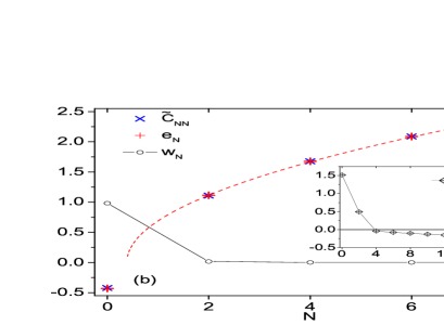
Figure 1: (Color online) (a).Effective scattering length $a_{\rm eff}/a_{0}$ as functions of $a_{0}/a_{s}$ for ⁴¹K(2D)-⁸⁷Rb(3D) mixture. The dashed line denotes the first resonance at $a_{0}/a_{s}=-0.43$. (b)Diagonal matrix element $\tilde{C}_{NN}$ of Eq.84(denoted by $\times$), the corresponding resonance position $(a_{0}/a_{s})_{res}$($+$) and resonance width($\circ$). Red dashed line is the function fit according to Eq.39. Inset shows the relative correction $\Delta_{N}$ as defined in Eq.38. $N=0,2,4...$ in (b) respectively correspond to the $(N/2+1)-$th induced resonance in (a) from left to right.

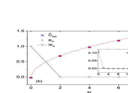
Figure 2: (Color online) Same as Fig.1 except for ⁴⁰K(2D)-⁶Li(3D) mixture. The dashed line in (a) denotes the first resonance at $a_{0}/a_{s}=-0.02$.

In addition, Fig.1 and Fig.2 show that the first resonance, which is mainly due to the coupling between relative motion levels within the lowest molecular channel($N=0$), always occurs at $a_{s}<0$ side regardless of $u>1$ or $u<1$. The resonance position, however, sensitively depends on the value of $u$, as shown by the vertical dashed lines in Fig.1(a) and Fig.2(a). This phenomenon is closely related to the distinct behaviors of $\tilde{C}_{NN}$ for different $u$. On one hand, when $u\ll 1$ we can omit the $n_{A}$-dependence in $\ln-$function in Eq.84, then using Eq.83 we obtain $\tilde{C}_{NN}\rightarrow 0$ for any $N$. This implies that when trapping the heavy atom, the resonance positions [$(a_{0}/a_{s})_{res}$] tend to highly aggregate around unshifted position($a_{0}/a_{s}=0$). On the other hand, when $u\gg 1$, $f_{N;n_{A},k_{z}}$ is vanishingly small for finite $N$, then the first term dominates in Eq.84. This predicts resonances approaching $a_{s}=0^{-}$. Only for large enough $N$ the rest terms in Eq.84 would dominate and predict resonances at $a_{s}>0$ side.

We note that the dependence of the first resonance position (at $a_{s}<0$ side) on the mass ratio $u$ is in qualitative agreement with that for 0D-3D mixturesCastin . Actually we can gain the physical insight of such feature from the analysis of interaction potentials affected by the confinement. Suppose a square-well interaction potential $U(r)$, which is $-V_{0}$ at $r<r_{0}$ and zero otherwise, between A and B atoms. As $V_{0}$ increases, the first scattering resonance occurs at the critical value $V_{c}=(\pi/2)^{2}/(2\mu r_{0}^{2})$ with $\mu$ the reduced mass. When A or B is trapped and becomes localized, $\mu$ will be effectively enhanced, which reduces the critical $V_{c}$ and gives new resonance at $a_{s}<0$ side. $\mu$ and $V_{c}$ can be substantially modified if the lighter atom is trapped, and the resonance position will move far away to $a_{s}=0^{-}$ side. On the contrary, if the heavier atom is trapped, $\mu$ and $V_{c}$ would be little affected by the trapping potential, giving almost unshifted resonance near $a_{s}=\infty$. This analysis leads to similar conclusions for the resonance scattering in other mixed-dimensional systems, such as 1D-3D mixtures.

IV Application to three-body problem

Besides the two-body system, the general formulism of T-matrix approach allows its straightforward extension to other few-body systems. In this section we focus on a three-body system composed by two-component fermions in a (rotating) harmonic trap. We shall first present the formulism and then explore the interesting scattering property and identify the ground state level crossing in this system.

IV.1 Formulism

We consider three fermions with one spin-$\downarrow$ ($\mathbf{x}_{1}$) and two identical spin-$\uparrow$ ($\mathbf{x}_{2},\mathbf{x}_{3}$) in an isotropic harmonic trap. According to Eqs.(65-68), we transform the vector $\mathbf{X}=(\sqrt{2m_{\downarrow}}\mathbf{x}_{1},\sqrt{2m_{\uparrow}}\mathbf{x}_{2},\sqrt{2m_{\uparrow}}\mathbf{x}_{3})$ to $\mathbf{Y_{\pm}}=(\sqrt{2M_{R}}\mathbf{R},\sqrt{2\mu}\mathbf{r}_{\pm},\sqrt{2\mu}\boldsymbol{\rho}_{\pm})$ by $\mathbf{Y_{\pm}}^{T}=A_{\pm}\mathbf{X}^{T}$. Here $(\mathbf{R},\mathbf{r}_{-},\boldsymbol{\rho}_{-})$ and $(\mathbf{R},\mathbf{r}_{+},\boldsymbol{\rho}_{+})$ are all Jacobi coordinates, respectively corresponding to the effective mass $M_{R},\mu,\mu$; the CM coordinate $\mathbf{R}$ and its mass $M_{R}$ follow Eq.66; the other Jacobi coordinates are

$$\mathbf{r_{-}} = \mathbf{x}_{2}-\mathbf{x}_{1},$$

$$\boldsymbol{\rho}_{-} = \frac{\sqrt{Mm_{\downarrow}}}{m_{\uparrow}+m_{\downarrow}}[\mathbf{x}_{3}-\frac{m_{\downarrow}\mathbf{x}_{1}+m_{\uparrow}\mathbf{x}_{2}}{m_{\uparrow}+m_{\downarrow}}],$$ (40)

with the same mass $\mu=\frac{m_{\uparrow}m_{\downarrow}}{m_{\uparrow}+m_{\downarrow}}$; the transfer matrix reads

$$A_{-}=\left(\begin{array}[]{ccc}\sqrt{\frac{m_{\downarrow}}{M}}&\sqrt{\frac{m_{\uparrow}}{M}}&\sqrt{\frac{m_{\uparrow}}{M}}\\ -\sqrt{\frac{m_{\downarrow}}{m_{\uparrow}+m_{\downarrow}}}&\sqrt{\frac{m_{\uparrow}}{m_{\uparrow}+m_{\downarrow}}}&0\\ -\frac{m_{\uparrow}}{\sqrt{M(m_{\uparrow}+m_{\downarrow})}}&-\sqrt{\frac{m_{\uparrow}m_{\downarrow}}{M(m_{\uparrow}+m_{\downarrow})}}&\sqrt{\frac{m_{\uparrow}+m_{\downarrow}}{M}}\end{array}\right);$$ (41)

we further obtain $\boldsymbol{\rho}_{+},\mathbf{r_{+}}$ by exchanging $\mathbf{x}_{2}\leftrightarrow\mathbf{x}_{3}$ in $\mathbf{r_{-}},\boldsymbol{\rho}_{-}$, and obtain $A_{+}$ by exchanging the second and third column of $A_{-}$.

Taking advantage of the property of transfer matrix (Eq.69), we can see that with the same trapping frequency $\omega$, all three Jacobi coordinates $(\mathbf{R},\mathbf{r}_{\pm},\boldsymbol{\rho}_{\pm})$ can be well separated from each other. Independently one can also prove that the total angular momentum is also separable as $\sum_{i=1,2,3}\hat{L}_{\alpha}(\mathbf{x}_{i})=\hat{L}_{\alpha}(\mathbf{R})+\hat{L}_{\alpha}(\boldsymbol{\rho}_{\pm})+\hat{L}_{\alpha}(\mathbf{r}_{\pm})\ (\alpha=x,y,z)$. Therefore for a trapped system with rotating frequency $\Omega$ around z-direction, the relevant Hamiltonian in the rotating frame reads

$$H(\boldsymbol{\rho}_{\pm},\mathbf{r_{\pm}})=H_{0}(\boldsymbol{\rho}_{\pm})+H_{0}(\mathbf{r_{\pm}})+U_{0}\delta(\mathbf{r_{+}})+U_{0}\delta(\mathbf{r_{-}}),$$ (42)

here

$$H_{0}(\mathbf{r})=-\frac{\nabla^{2}_{\mathbf{r}}}{2\mu}+\frac{1}{2}\mu\omega^{2}\mathbf{r}^{2}-\Omega L_{z}(\mathbf{r}).$$ (43)

The molecular state is defined with respect to Fermi statistics,

$$|\lambda\rangle=\frac{1}{\sqrt{2}}(|r_{-}=0,\lambda\rangle-|r_{+}=0,\lambda\rangle).$$ (44)

Here the first and second $\lambda$ represent the identical energy level $\{nlm\}$ for the motions of $\boldsymbol{\rho}_{-}$ and $\boldsymbol{\rho}_{+}$ under Hamiltonian $H_{0}$. ($\{n\}$ and $\{lm\}$ are respectively the radial and azimuthal quantum number). Then we obtain the $C-$matrix element as

$$C_{\mathbf{\lambda\lambda^{\prime}}}=(\frac{1}{V}\sum_{\mathbf{k}}\frac{1}{\epsilon_{\mathbf{k}}}+\sum_{\nu}\frac{|\psi_{\nu}(0)|^{2}}{E-E_{\lambda}-E_{\nu}+i\delta})\delta_{\lambda\lambda^{\prime}}-F_{\lambda\lambda^{\prime}},$$ (45)

with

$$F_{\lambda\lambda^{\prime}} = \langle r_{-}=0,\lambda|\hat{G}_{0}|r_{+}=0,\lambda^{\prime}\rangle$$ (46)

$$= \int d\boldsymbol{\rho}\psi^{*}_{\lambda}(\boldsymbol{\rho})\psi_{\lambda^{\prime}}(-\beta\boldsymbol{\rho})\sum_{\nu}\frac{\psi_{\nu}(0)\psi_{\nu}(-\alpha\boldsymbol{\rho})}{E-E_{\lambda^{\prime}}-E_{\nu}+i\delta},$$

here

$$\alpha=\frac{\sqrt{Mm_{\downarrow}}}{m_{\uparrow}+m_{\downarrow}},\ \ \ \ \beta=\frac{m_{\uparrow}}{m_{\uparrow}+m_{\downarrow}},$$ (47)

and $\alpha^{2}+\beta^{2}=1$. To obtain Eq.46 we have inserted into the Green function a complete set of eigen-states $\{\nu,\lambda^{\prime}\}$ for the motions of $(\mathbf{r}_{+},\boldsymbol{\rho}_{+})$. $F_{\lambda\lambda^{\prime}}=F^{*}_{\lambda^{\prime}\lambda}$ here induce the coupling between different molecular levels, and non-zero $F_{\lambda\lambda^{\prime}}$ require azimuthal quantum number $\{lm\}$ be conserved. Note that the off-diagonal coupling of molecular states here is due to the many-body statistics, in contrary to the previous two-body case which is due to the external trapping potentials. More details regarding to the evaluation of Eq.45 are presented in Appendix D.

IV.2 Results

In the first part of this section we use T-matrix method to analyze the exotic scattering property of three fermions in different limits of mass ratios and in different angular momenta channels. In the second part, we present the energy spectrum and identify the energy level crossing between different angular momenta states for the (rotating) trapped system.

IV.2.1 Scattering property

By analyzing Eqs.(45,46), we find nontrivial scattering properties at two limits of mass ratio $u=m_{\uparrow}/m_{\downarrow}$. Fig.3 shows the schematic plots of Jacobi coordinates $(\mathbf{r}_{-},\boldsymbol{\rho}_{-})$ in both limits of $u\rightarrow 0$ and $u\rightarrow\infty$.

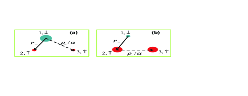
Figure 3: (Color online) Jacobi coordinates $(\mathbf{r}_{-},\boldsymbol{\rho}_{-})$ for three fermions($\uparrow\uparrow\downarrow$) in the limit of $u\rightarrow 0$ (a) and $u\rightarrow\infty$ (b). $u=m_{\uparrow}/m_{\downarrow}$ is the mass ratio. $\alpha$ is given by Eq.47.

First, when $u\rightarrow 0$ as shown by Fig.3(a), $\alpha\rightarrow 1,\ \beta\rightarrow 0$, we have

$$F_{\lambda\lambda^{\prime}}\sim\delta_{l,0}\delta_{l^{\prime},0}.$$ (48)

Therefore the diagonal C-matrix for $l\neq 0$ indicates the atom-dimer uncorrelated system with energy $E=E_{a}+E_{d}$. Physically we can see from Fig.3(a) that, the dimer formed by a light $\uparrow$ and heavy $\downarrow$ is almost equivalent to single $\downarrow$ atom, so the other $\uparrow$ has s-wave interaction with this dimer only when $l=0$. Here the heavy $\downarrow$ dominates the whole physics.

Second, in the opposite limit when $u\rightarrow\infty$ as shown by Fig.3(b), the result is completely different. We find in this limit,

$$C_{\mathbf{\lambda\lambda^{\prime}}}=(-\frac{1}{V}\sum_{\mathbf{k}}\frac{1}{\epsilon_{\mathbf{k}}}-\sum_{\nu}\frac{|\psi_{\nu}(0)|^{2}}{E-E_{\lambda}-E_{\nu}+i\delta}[1-(-1)^{l}])\delta_{\lambda\lambda^{\prime}}.$$ (49)

There are two direct consequences as follows.

(i)for odd $l$, $C_{\mathbf{\lambda\lambda^{\prime}}}=\infty$, i.e., unphysical divergence in the high-energy space can not be properly removed. This is exactly the evidence of Efimov effect for large $u$ where another short-range parameter is required to help fix the three-body problemEfimov ; Braaten06 .

(ii)for even $l$, $\hat{U}$ takes no effect and the system just behaves like non-interacting. This result is consistent with that obtained by Born-Oppenheimer approximation(BOA)NPA1979 . Under BOA, the wavefunction is given by

$$\psi(\mathbf{x}_{1},\mathbf{x}_{2},\mathbf{x}_{3})=[\varphi(|\mathbf{x}_{2}-\mathbf{x}_{1}|)+\gamma\varphi(|\mathbf{x}_{3}-\mathbf{x}_{1}|)]f(\mathbf{x}_{2},\mathbf{x}_{3}),$$ (50)

where the first part describes the light particle moving around two static heavy particles, and $f(\mathbf{x}_{2},\mathbf{x}_{3})$ describes for two heavy particles afterwards. By imposing Bethe-Peierls boundary conditions one can find $\gamma=\pm 1$, and the energy of the first part just depends on $|\mathbf{x}_{2}-\mathbf{x}_{3}|$. Therefore the wavefunction is reduced to

$$\psi(\mathbf{x}_{1},\mathbf{x}_{2},\mathbf{x}_{3})=[\varphi(\mathbf{|r_{-}|})\pm\varphi(\mathbf{|r_{+}|})]f_{1}(\mathbf{x}_{2}-\mathbf{x}_{3})f_{2}(\mathbf{R}),$$ (51)

and then angular momentum $l$ is determined only by $f_{1}(\mathbf{x}_{2}-\mathbf{x}_{3})$. For $\gamma=1$, the Fermi statistics require $l$ be odd; for $\gamma=-1$, $l$ is even but in this case one can easily check that the resultant wavefunction automatically get rid of the interaction, i.e., $\hat{U}\psi=0$. Here Fermi statistics of two $\uparrow$ spins take the crucial role.

Note that the results presented in (i,ii) uniquely benefit from the concept of renormalization and the procedure in momentum space to eliminate the ultraviolet divergence. These analyses of scattering properties for different mass ratios and different angular momenta will be helpful to understand the ground state level crossing in the following section.

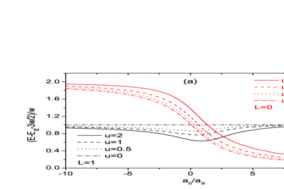
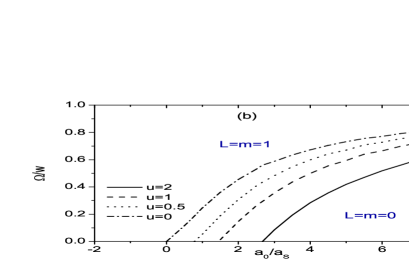
Figure 4: (Color online) (a).Energy of three fermions($\uparrow\uparrow\downarrow$) vs interaction strength in a non-rotating isotropic harmonic trap, with $a_{0}=\sqrt{1/(\mu\omega)}$ the confinement length. Different mass ratios $u=m_{\uparrow}/m_{\downarrow}$ for total angular momentum $l=0$(red) and $l=1$(black) are plotted. The energy is shifted by the ground-state atom-dimer energy, $E_{d}+3\omega/2$($E_{d}$ is the dimer energy). (b)Phase diagram in a rotating harmonic trap with rotating frequency $\Omega$. The ground state is $|l=m=1\rangle$ above the curves and $|l=m=0\rangle$ below.

IV.2.2 Energy level crossing

First, we identify the energy level crossing between different angular momenta states for a non-rotating system. The energy spectrum of a non-rotating system was previously studied for equal massDuan07 ; Liu10 , and unequal masses using Gaussian expansion techniqueStecher08 and adiabatic hyperspherical methodRittenhouse10 . In Fig.4(a) we show the spectrum for angular momenta $l=0,1$ and for different mass ratios using T-matrix method. We also checked for higher $l\geq 2$ and confirm those states are less modified by the interaction and thus not shown here.

The system in weak interacting limit($a_{s}\rightarrow 0^{-}$) behaves as non-interacting while in molecule limit($a_{s}\rightarrow 0^{+}$) as a single dimer plus an atom. This directly results in the inversion of ground state from angular momentum $l=1$ to $l=0$ as $1/a_{s}$ increases. As shown in Fig.4(a), the inversion is denoted by the energy level crossing, and the position of level crossing closely depends on mass ratio $u$. As expected, when $u$ increases from $0$ to $\infty$, all energy levels with even-$l$ move upwards and the system evolves from decoupled atom-dimer(except for $l=0$) to three atoms that are immune from interactions; while all odd-$l$ move downwards until Efimov physics show up and invalidate the present T-matrix method. Therefore by increasing $u$, the position of level crossing will move to strong coupling side as shown in Fig.4(a). Intuitively, one can also attribute this to the enhanced s-wave repulsion between atom and dimerPetrov1 .

In unitary limit, our numerical results are in good accordance with those obtained by using hyperspherical coordinates. Previously, hyperspherical coordinate method has been applied to a trapped system with equal massWerner061 ; Werner062 . In Appendix E we extend this method to arbitrary mass ratios. Note that the maximum mass ratio considered in Fig.3 is much less than critical value, $u_{c}=13.6$Petrov1 , for the emergence of Efimov state in $l=1$ channel (as also predicted by Eq.96 when setting $s=0$). In this regime, as the matrix size increases we get convergent result for the energy spectrum.

Finally, we present the ground state for the trapped system with rotation($\Omega>0$). By comparing energies of all different angular momenta $l$ we obtain the ground state as shown in Fig.4(b). We find $l=m=1$ state is gradually favored by the rotation. The energy gain of this state is analyzed to be partly from the reduction of kinetic energy with respect to $l=0$, and partly from the avoided s-wave repulsion between atom and dimer. As $\Omega$ increases, the system evolves to the atom-dimer quantum Hall state; particularly at $\Omega=\omega$, all states with odd-$l$ degenerate. Finally we expect above quantum Hall physics of fermionic system could be studied in experiment, as recently realized in a rotating few-body bosonic systemGemelke10 .

V Summary

In conclusion, we present a systematic T-matrix approach to solve few-body problems with contact interactions in the field of ultracold atoms. Taking advantage of zero-range interactions, the key ingredient of the present T-matrix method is to project the problem to a subspace that is expanded by orthogonal molecular states, and meanwhile take careful considerations of the renormalization for relative motions. This method successfully unifies the calculations of various physical quantities in a single framework, including the bound state solutions, effective scattering lengths and reduced interactions in the lower dimension.

We present two applications of this approach, namely, two-body scattering resonances in 2D-3D mixed dimensions and properties of three fermions($\uparrow\uparrow\downarrow$) in a 3D (rotating) trap. For the two-body problem, we show that T-matrix provides a physically transparent way to understand the mechanism of induced scattering resonances. Besides, it also gives explicit expressions for the resonance positions and widths. Due to the separate treatment of relative motions from CM motions, each resonance can be determined accurately by only considering a few related matrix elements. For the three-body problem, T-matrix enables us to identify exotic scattering properties of three fermions in different angular momentum channels and with different mass ratios. In a rotating system, these properties provide important hints for the quantum Hall transition from zero to finite angular momentum state. Overall, the external confinements, mass ratios, and bosonic/fermionic statistics all play important roles and give rise to very rich phenomenon in these few-body systems.

The author thanks Hui Zhai, Shina Tan, Fei Zhou, Hui Hu and Doerte Blume for useful discussions, and Jason Ho for valuable suggestions on the manuscript. This work is supported by Tsinghua University Basic Research Young Scholars Program and Initiative Scientific Research Program and NSFC under Grant No. 11104158. The author would like to thank the hospitality of the Institute for Nuclear Theory at University of Washington, where this work is finally completed during the workshop on ”Fermions from Cold Atoms to Neutron Stars” in the spring of 2011.

Appendix A Construction of individual molecular state

In this appendix, we show how to construct an individual molecular state in the most efficient way. Let us consider a system of $N$ particles with masses $m_{1},...m_{N}$ and coordinates $\mathbf{x}_{1},...\mathbf{x}_{N}$. For a general case, the molecular state is written as

$$|\mathbf{x}_{1}=\mathbf{x}_{2},\lambda=\{N,n_{3},n_{4},...n_{N}\}\rangle.$$ (52)

In coordinate space it can be factorized as $\Phi_{N}(\mathbf{X})\prod_{i=3}^{N}\phi_{n_{i}}(\mathbf{x}_{i})$, where $\phi_{n_{i}}(\mathbf{x}_{i})$ is the eigen-state of single-particle Hamiltonian

$$\hat{H}_{0}(\mathbf{x}_{i})=-\frac{\nabla_{\mathbf{x}_{i}}^{2}}{2m_{i}}+V_{T,i}(\mathbf{x}_{i})$$ (53)

and $\Phi_{N}(\mathbf{X})$ the eigen-state of

$$\hat{H}_{0}(\mathbf{X})=-\frac{\nabla_{\mathbf{X}}^{2}}{2(m_{1}+m_{2})}+V_{T,2}(\mathbf{X})+V_{T,2}(\mathbf{X}).$$ (54)

Here $V_{T,i}$ is the trapping potential for the $i-$th particle. The overlap between the molecular state(Eq.52) and N-particle state($\prod^{N}_{j=1}|l_{j}\rangle$) is

$$\langle\mathbf{x}_{1}=\mathbf{x}_{2},\lambda|l_{1},l_{2},l_{3},...l_{N}\rangle=\gamma_{N;l_{1},l_{2}}\prod_{i=3}^{N}\delta_{n_{i}l_{i}}$$ (55)

with

$$\gamma_{N;l_{1},l_{2}}=\int d\mathbf{X}\Phi_{N}^{*}(\mathbf{X})\phi_{l_{1}}(\mathbf{X})\phi_{l_{2}}(\mathbf{X}).$$ (56)

The Green function term in Eq.11 can then be computed efficiently as

$$\langle r_{I}=0,\lambda|\hat{G}_{0}(E)|r_{I^{\prime}}=0,\lambda^{\prime}\rangle$$ (57)

$$= \sum_{l_{1}...l_{N}}\frac{\langle r_{I}=0,\lambda|l_{1}...l_{N}\rangle\langle l_{1}...l_{N}|r_{I^{\prime}}=0,\lambda^{\prime}\rangle}{E-(E_{l_{1}}+...+E_{l_{N}})+i\delta}.$$

To this end we have shown a general way to construct an individual molecular state. Furthermore, for special trapping potentials which enable the decoupling of CM motion from other motions, it is convenient to remove the CM motion from the problem and transform the effective coordinate vector

$$\mathbf{X}=(\sqrt{2m_{1}}\mathbf{x}_{1},\sqrt{2m_{2}}\mathbf{x}_{2},\sqrt{2m_{3}}\mathbf{x}_{3},...\sqrt{2m_{N}}\mathbf{x}_{N})$$ (58)

to the Jacobi coordinates

$$\mathbf{Y}=(\sqrt{2M_{R}}\mathbf{R},\sqrt{2\mu}\mathbf{r},\sqrt{2\nu_{1}}\boldsymbol{\rho}_{1},...\sqrt{2\nu_{N-2}}\boldsymbol{\rho}_{N-2})$$ (59)

by a matrix equation

$$\mathbf{Y}^{T}=A\mathbf{X}^{T},$$ (60)

with A-matrix element

$$A_{ij}=\left\{\begin{array}[]{l}\sqrt{m_{j}/M_{N}},\ \ (i=1)\\ \sqrt{M_{i-1}/M_{i}},\ \ (i=j>1)\\ -\sqrt{m_{i}m_{j}/(M_{i-1}M_{i})},\ \ (i>j\geq 1)\\ 0,\ \ \textrm{all else}\end{array}\right.$$ (65)

here $M_{j}=\sum_{i=1}^{j}m_{i}$.

For the CM motion, we have the coordinate and the mass

$$\mathbf{R}=\sum_{i=1}^{N}\frac{m_{i}\mathbf{x}_{i}}{M_{N}},\ \ \ M_{R}=\sum_{i=1}^{N}m_{i};$$ (66)

for other motions, we take the unique choice as

$$\sqrt{2\mu}\mathbf{r} = \sqrt{\frac{2m_{1}m_{2}}{m_{1}+m_{2}}}(\mathbf{x}_{2}-\mathbf{x}_{1}),$$ (67)

$$\sqrt{2\nu_{j}}\boldsymbol{\rho}_{j} = \sqrt{\frac{2m_{i+2}M_{i+1}}{M_{i+2}}}(\mathbf{x}_{j+2}-\sum_{i=1}^{j+1}\frac{m_{i}\mathbf{x}_{i}}{M_{j+1}}).$$ (68)

According to Eq.65, A-matrix satisfies

$$AA^{T}=A^{T}A=I,$$ (69)

here $I$ is identity matrix; this gives

$$d\mathbf{R}d\mathbf{r}\prod^{N-2}_{j}d\rho_{j}=\prod^{N}_{i}d\mathbf{x}_{i}$$ (70)

and

$$\nabla_{\mathbf{X}}\nabla^{T}_{\mathbf{X}}=\nabla_{\mathbf{Y}}\nabla^{T}_{\mathbf{Y}},\ \ \mathbf{X}\mathbf{X}^{T}=\mathbf{Y}\mathbf{Y}^{T}.$$ (71)

Therefore $M_{R},\mu,\nu_{1},...\nu_{N-2}$ can be considered as the effective mass respectively for the motion of $\mathbf{R},\mathbf{r},\boldsymbol{\rho}_{1},...\boldsymbol{\rho}_{N-2}$. By decomposing the trapping potential to be

$$\sum_{i}V_{T,i}(\mathbf{x}_{i})=V_{T}(\mathbf{R})+V_{T}(\mathbf{r},\boldsymbol{\rho}_{1},...\boldsymbol{\rho}_{N-2}),$$ (72)

we choose the molecular state $|r=0,\lambda\rangle$ such that its real-space wavefunction $\phi_{\lambda}(\boldsymbol{\rho}_{1},...\boldsymbol{\rho}_{N-2})$ is the eigen-state of the following Hamiltonian for $N-2$ particles

$$\hat{H}^{N-2}_{0}=-\sum_{j=1}^{N-2}\frac{\nabla_{\boldsymbol{\rho}_{j}}^{2}}{2\nu_{j}}+V_{T}(r=0,\boldsymbol{\rho}_{1},...\boldsymbol{\rho}_{N-2}).$$ (73)

The Green function in Eq.11 is obtained by inserting eigen-states of the following Hamiltonian for $N-1$ particles

$$\hat{H}^{N-1}_{0}=-\frac{\nabla_{\mathbf{r}}^{2}}{2\mu}-\sum_{j=1}^{N-2}\frac{\nabla_{\boldsymbol{\rho}_{j}}^{2}}{2\nu_{j}}+V_{T}(\mathbf{r},\boldsymbol{\rho}_{1},...\boldsymbol{\rho}_{N-2}).$$ (74)

Compared with Eq.(52-57) for a general case, the degree of freedom here is further reduced by one particle.

Appendix B Derivation of Eq.10

To facilitate the derivation of Eq.10, we assume there is only one pair of particles interacting with $U_{I}\delta^{3}(\mathbf{r}_{I})$, and we have

$$\langle\mathbf{r}_{I},\lambda|\hat{U}=U_{I}\delta^{3}(\mathbf{r}_{I})\langle r_{I}=0,\lambda|.$$ (75)

Using the Lippmann-Schwinger equation or equivalently

$$T=U+UG_{0}T,$$ (76)

and together with Eq.9 we obtain

$$\sum_{I^{\prime}\lambda^{\prime}}f^{I^{\prime}}_{\lambda^{\prime}}|r_{I^{\prime}}=0,\lambda^{\prime}\rangle=U|\psi_{0}\rangle+UG_{0}\sum_{I^{\prime}\lambda^{\prime}}f^{I^{\prime}}_{\lambda^{\prime}}|r_{I^{\prime}}=0,\lambda^{\prime}\rangle.$$ (77)

The inner product with $\langle r_{I}=0,\lambda_{I}|$ gives

$$\sum_{I^{\prime}\lambda^{\prime}}f^{I^{\prime}}_{\lambda^{\prime}}(\frac{1}{U_{I}}\delta_{II^{\prime}}\delta_{\lambda\lambda^{\prime}}-\langle r_{I}=0,\lambda|\hat{G}_{0}|r_{I^{\prime}}=0,\lambda^{\prime}\rangle)$$

$$\ \ \ \ \ \ \ \ =\langle r_{I}=0,\lambda|\psi_{0}\rangle.$$ (78)

Here we have extracted the most singular terms as characterized by $\delta^{3}(\mathbf{r}_{I})$. After further renormalizing the bare interaction $U_{I}$ we obtain Eq.10.

Above derivation can be generalized to the case when the molecular state $|r_{I}=0,\lambda_{I}\rangle$ is the superposition of many individual ones according to bosonic or fermionic statistics. After a proper combination of the resulted individual equations, one can equally obtain Eq.10.

Appendix C Effective scattering in 2D-3D mixture

In this appendix we study two-body scattering in 2D-3D mixed dimensions(see also Section IIIB).

First, we relate the effective scattering length to T-matrix element between zero-energy scattering states. From Eq.1, the two-body wavefunction in coordinate space reads

$$\psi(\boldsymbol{\rho}_{AB},z_{A},z_{B})=\psi_{0}(\boldsymbol{\rho}_{AB},z_{A},z_{B})+\sum_{n_{A}}\sum_{\mathbf{k}_{\rho},k_{z}}\phi_{n_{A}}(z_{A},a_{0})$$

$$\frac{1}{\sqrt{V}}\frac{e^{i\mathbf{k}_{\rho}\cdot\boldsymbol{\rho}_{AB}}e^{ik_{z}z_{B}}}{E-n_{A}\omega_{A}-\frac{\mathbf{k}_{\rho}^{2}}{2\mu}-\frac{k_{z}^{2}}{2m_{B}}+i\delta}\langle\mathbf{k}_{\rho},n_{A},k_{z}|T|\psi_{0}\rangle,$$ (79)

with $\boldsymbol{\rho}_{AB}$ the relative coordinate of A and B in xy plane and $z_{A},z_{B}$ their respective coordinate in z-direction; $E$ is counted from the zero-point energy $\omega_{A}/2$. For large separations, both $e^{i\mathbf{k}_{\rho}\cdot\boldsymbol{\rho}_{AB}}$ and $e^{ik_{z}z_{B}}$ oscillate far more rapidly in k-space than T-matrix term. Thus in the limits of $E\rightarrow 0^{+}$ and $|\boldsymbol{\rho}_{AB}|,\ |z_{B}|\rightarrow\infty$, we can specify $\mathbf{k}_{\rho}=0,\ k_{z}=0$ in all T-matrix elements and reduce Eq.79 to

$$\psi(\boldsymbol{\rho}_{AB},z_{A},z_{B})\rightarrow\phi_{0}(z_{A})(1-\frac{\mu}{2\pi d_{AB}}V\langle\psi_{0}|T|\psi_{0}\rangle)$$

$$\ \ -\sum_{n_{A}>0}\phi_{n_{A}}(z_{A},a_{0})\frac{\mu}{2\pi d_{AB}}e^{-\kappa_{n_{A}}d_{AB}}V\langle 0,n_{A},0|T|\psi_{0}\rangle$$

$$\rightarrow\phi_{0}(z_{A},a_{0})(1-\frac{a_{\rm eff}}{d_{AB}}),\ \ \ (d_{AB}\rightarrow\infty)$$ (80)

with $\kappa_{n_{A}}=\sqrt{2m_{B}n_{A}\omega_{A}}$, $d_{AB}=\sqrt{\frac{\mu}{m_{B}}\boldsymbol{\rho}_{AB}^{2}+z_{B}^{2}}$, and $a_{\rm eff}$ directly related to T-matrix element as given by Eq.34.

In Eq.36, $e_{\nu}$ and $W_{N}$ can be obtained from the diagonalization of the following matrix

$$\tilde{C}_{NN^{\prime}} = \frac{2\pi a_{0}}{\mu}\Big{\{}\frac{1}{V}\sum_{\mathbf{k}}\frac{1}{\mathbf{k}^{2}/(2\mu)}\delta_{NN^{\prime}}+$$ (81)

$$\sum_{n_{A}}\sum_{k_{z},\mathbf{k}_{\rho}}\frac{1}{V}\frac{f_{N;n_{A},k_{z}}f^{*}_{N^{\prime};n_{A},k_{z}}}{E-n_{A}\omega_{A}-\frac{\mathbf{k}_{\rho}^{2}}{2\mu}-\frac{k_{z}^{2}}{2m_{B}}+i\delta}\Big{\}},$$

with

$$f_{N;n_{A},k_{z}}=\int_{-\infty}^{+\infty}dZ\phi^{*}_{N}(Z,\overline{a})\phi_{n_{A}}(Z,a_{0})e^{ik_{z}Z}.$$ (82)

Using the exact identity

$$\sum_{n_{A}}|f_{N;n_{A},k_{z}}|^{2}=1,$$ (83)

we eliminate the logarithmic divergence when summing over $\mathbf{k}_{\rho}$ and finally simplify Eq.81 to be

$$\tilde{C}_{NN^{\prime}} = \frac{1}{\pi}\int_{0}^{\infty}d\tilde{k}_{z}\Big{\{}-\ln(\tilde{k}_{z}^{2})\delta_{NN^{\prime}}+\sum_{n_{A}}$$ (84)

$$f_{N;n_{A},k_{z}}f^{*}_{N^{\prime};n_{A},k_{z}}\ln(\frac{\tilde{k}_{z}^{2}}{1+u}+n_{A}\frac{2u}{1+u})\Big{\}}.$$

In practical calculations, we set the cutoff of $n_{A}$ to be $1000$ for K-Rb($m_{A}<m_{B}$) and $700$ for K-Li($m_{A}>m_{B}$) mixture, depending on the convergence in terms of $n_{A}$ in each case. The cutoff of $\tilde{k}_{z}(=k_{z}a_{0})$ is chosen within $20\sim 30$ to check the insensitive dependence on the cutoff and ensure the accuracy of the integration.

Appendix D Evaluation of Eq.45

The eigen-state of Hamiltonian (Eq.43) is

$$\psi_{nlm}(r,\theta,\phi)=\mathcal{N}_{nl}a_{0}^{-3/2}(\frac{r}{a_{0}})^{l}e^{-r^{2}/(2a_{0}^{2})}L_{n}^{l+\frac{1}{2}}(\frac{r^{2}}{a_{0}^{2}})Y_{lm}(\theta,\phi)$$ (85)

where $\mathcal{N}_{nl}=\sqrt{\frac{2n!}{\Gamma(n+l+3/2)}}$, $a_{0}=\sqrt{1/(\mu w)}$; $L_{n}^{l+\frac{1}{2}}$ is the generalized Laguerre polynomial; the corresponding eigen-energy is $E_{nlm}=(2n+l+\frac{3}{2})\omega-m\Omega$.

The eigen-solution($E$) of the interacting system is determined by Eq.12, or equivalently (for given $\{lm\}$)

$$Det(\frac{a_{0}}{a_{s}}\delta_{nn^{\prime}}-\tilde{C}_{nn^{\prime}})=0,$$ (86)

where $\tilde{C}_{nn^{\prime}}=A_{n}\delta_{nn^{\prime}}-\tilde{F}_{nn^{\prime}}$, with

$$A_{n}=\lim_{\Lambda\rightarrow\infty}\Big{[}\frac{4\sqrt{\Lambda}}{\pi}+\sum_{n^{\prime\prime}=0}^{\Lambda}\frac{\frac{2}{\sqrt{\pi}}\frac{(2n^{\prime\prime}+1)!!}{(2n^{\prime\prime})!!}}{\tilde{E}-\tilde{E}_{nlm}-\tilde{E}_{n^{\prime\prime}00}}\Big{]},$$ (87)

$$\tilde{F}_{nn^{\prime}}=\sum_{n^{\prime\prime}}\frac{B_{nn^{\prime}n^{\prime\prime}}}{\tilde{E}-\tilde{E}_{nlm}-\tilde{E}_{n^{\prime\prime}00}},$$ (88)

$$B_{nn^{\prime}n^{\prime\prime}} = (-\beta)^{l}\mathcal{N}_{nl}\mathcal{N}_{n^{\prime}l}\frac{2}{\sqrt{\pi}}\int_{0}^{\infty}dxx^{2l+2}e^{-x^{2}}$$ (89)

$$L_{n}^{l+\frac{1}{2}}(x^{2})L_{n^{\prime}}^{l+\frac{1}{2}}(\beta^{2}x^{2})L_{n^{\prime\prime}}^{\frac{1}{2}}(\alpha^{2}x^{2}).$$

Here $\tilde{E}=E/\omega$. In our numerical simulations, the typical size of the matrix for diagonalization is $50\times 50$. When sum over intermediate states, the actual cutoff of $n^{\prime\prime}$, namely $n^{c}$, depends on the values of $\{n,n^{\prime}\}$, which is constrained by $B_{nn^{\prime}n^{c}}\leq 10^{-4}$ in practical calculations.

Appendix E Unitary three-fermions with arbitrary mass ratios

In unitary limit, it is convenient to use hyperspherical coordinates to express the three-body wavefunctionBraaten06 ; Werner061 ; Werner062 as

$$\psi(\mathbf{r}_{\pm},\boldsymbol{\rho}_{\pm})=\frac{F(R)}{R^{2}}(1-P_{23})\frac{\varphi(\xi)}{\sin(2\xi)}Y_{lm}(\hat{\rho}_{-}),$$ (90)

with $\mathbf{r}_{\pm},\ \ \boldsymbol{\rho}_{\pm}$ given by Eq.40; $P_{23}$ is the permutation operator for identical fermions $2$ and $3$;

$$R=\sqrt{\frac{\mathbf{r}^{2}_{\pm}+\boldsymbol{\rho}^{2}_{\pm}}{2}},\ \ \ \ \xi=\arctan\frac{|\mathbf{r}_{-}|}{|\boldsymbol{\rho}_{-}|},$$ (91)

are respectively the hyperradius and hyperangle. Using this ansatz, we obtain two decoupled Schrodinger equations for $R$ and $\xi$,

$$\big{[}-\frac{\hbar^{2}}{4\mu}(\frac{d^{2}}{dR^{2}}+\frac{1}{R}\frac{d}{dR})+\frac{\hbar^{2}s^{2}}{4\mu R^{2}}+\mu\omega^{2}R^{2}\big{]}F(R)=EF(R);$$ (92)

$$\big{[}-\frac{d^{2}}{d\xi^{2}}+\frac{l(l+1)}{\cos^{2}\xi}\big{]}\varphi(\xi)=s^{2}\varphi(\xi).$$ (93)

On the other hand, the Bethe-Peierls boundary condition applying to Eq.90 gives

$$\varphi^{\prime}(0)-\frac{(-1)^{l}}{\alpha\beta}\varphi(\arccos\beta)=0,$$ (94)

with $\alpha,\ \beta$ given by Eq.47. Combined with Eq.93, Eq.94 generates the following equations for $l=0$ and $l=1$ (assuming all $s$ are real and positive),

$$s\cos(\frac{\pi}{2}s)+\frac{1}{\alpha\beta}\sin(s\arcsin\beta)=0,\ \ \ (l=0)$$ (95)

$$(1-s^{2})\sin(\frac{\pi}{2}s) = \frac{1}{\alpha\beta}[s\cos(s\arcsin\beta)-\frac{\alpha}{\beta}\sin(s\arcsin\beta)]$$ (96)

$$\ \ \ \ \ \ \ \ \ \ \ \ \ \ \ \ \ \ \ \ (l=1).$$

which are the most relevant equations to the phase transition discussed in Section IVB. For equal mass $\mu=m/2$, above equations reduce to those in Ref.Werner061 ; Werner062 .

Note that the validity of above assumption ($s>0$) in deriving Eqs.(95,96) closely depends on the mass ratio $u$ and the angular momentum $l$. For any given $l$, the hyperangular equation (93) and condition (94) provide the solutions for $s$, which has double degenaracy($s$ and $-s$). For $l=1$ channel, the zero-range model would provide universal energy solutions for $u<8.62$ (with $s>1$)Nishida . When $8.62<u<13.6\ (0<s<1)$, the energy solution will depend on the details of interacting potentials and 3-body resonance might happen by tuning the potentialsBlume_prl ; Blume_pra . When $u>13.6\ (s^{2}<0)$ the imaginary $s$ indicates the Efimov physics with infinite number of shallow trimersPetrov1 .

In the actual computation of energy spectrum using T-matrix, for nearly all mass ratios below $13.6$ one would get the energy spectrum with good convergence, as the matrix size of Eq.86 is increased. The signal of 3-body resonance(occurs around $u=12.3$ with $s=1/2$) is vanishing weak due to the infinitesimal width produced by zero-range modelBlume2 . Therefore in the regime of $u<13.6$ one can just consider the $s>0$ solution. Then the hyperradius equation (92) gives the energy $E=(2n+s+1)\omega$ with $n(=0,1...)$ a semi-positive integer. In the rotating frame, the energy is further shifted by $-m\Omega$, with $m$ the magnetic quantum number and $\Omega$ the rotating frequency.

References

- (1) Bloch, I., Dalibard, J., Zwerger, W.: Many-body physics with ultracold gases. Rev. Mod. Phys. 80, 885-964 (2008)
- (2) Giorgini, S., Pitaevskii, L.P., Stringari, S.: Theory of ultracold atomic Fermi gases. Rev. Mod. Phys. 80, 1215-1274 (2008)
- (3) Petrov, D.S.: Three-body problem in Fermi gases with short-range interparticle interaction. Phys. Rev. A 67, 010703(R) (2003)
- (4) Petrov, D.S., Salomon, C., Shlyapnikov, G.V.: Weakly bound dimers of fermionic atoms. Phys. Rev. Lett. 93, 090404 (2004)
- (5) Tan, S.: Large momentum part of fermions with large scattering length. Ann. Phys. (N.Y.) 323, 2971-2986 (2008)
- (6) Tan, S.: Generalized virial theorem and pressure relation for a strongly correlated Fermi gas. Ann. Phys. (N.Y.) 323, 2987-2990 (2008)
- (7) Tan, S.: Energetics of a strongly correlated Fermi gas. Ann. Phys. (N.Y.) 323, 2952-2970 (2008)
- (8) Stewart, J.T., Gaebler, J.P., Drake, T.E., Jin, D.S.: Verification of universal relations in a strongly interacting Fermi gas. Phys. Rev. Lett. 104, 235301 (2010)
- (9) Efimov, V.: Energy levels arising from resonant two-body forces in a three-body system. Phys. Lett. B 33, 563 (1973)
- (10) Braaten, E., Hammer, H.-M.: Universality in few-body systems with large scattering length. Phys. Rep. 428, 259-390 (2006)
- (11) Busch, T., Englert, B.-G., Rzazewski, K., Wilkens, M.: Two cold atoms in a harmonic trap. Found. Phys. 28, 549 (1998)
- (12) Olshanii, M.: Atomic scattering in the presence of an external confinement and a gas of impenetrable bosons. Phys. Rev. Lett. 81, 938 (1998)
- (13) Bergeman, T., Moore, M.G., Olshanii, M.: Atom-atom xcattering under cylindrical harmonic confinement: numerical and analytic studies of the confinement induced resonance. Phys. Rev. Lett. 91, 163201 (2003)
- (14) Moritz, H., Stöferle, T., Güenter, K., Köhl, M., Esslinger, T.: Confinement induced molecules in a 1D Fermi gas. Phys. Rev. Lett. 94, 210401 (2005)
- (15) Petrov, D.S., Holzmann M., Shlyapnikov, G.V.: Bose-Einstein Condensation in quasi-2D trapped gases. Phys. Rev. Lett. 84, 2551 (2000)
- (16) Petrov, D.S., Shlyapnikov, G.V.: Interatomic collisions in a tightly confined Bose gas. Phys. Rev. A. 64, 012706 (2001)
- (17) Kestner J.P., Duan, L.-M.: Effective low-dimensional Hamiltonian for strongly interacting atoms in a transverse trap. Phys. Rev. A 76, 063610 (2007)
- (18) Orso, G., Pitaevskii, L.P., Stringari S., Wouters, W.: Formation of molecules near a Feshbach Resonance in a 1D optical lattice. Phys. Rev. Lett. 95, 060402 (2005)
- (19) Büchler, H.P.: Microscopic derivation of hubbard parameters for cold atomic gases. Phys. Rev. Lett. 104, 090402 (2010)
- (20) Cui, X., Wang Y.P., Zhou, F.: Resonance scattering in optical lattices and molecules: interband versus intraband effects. Phys. Rev. Lett. 104, 153201 (2010)
- (21) Peano, V., Thorwart, M., Mora C., Egger, R.: Confinement-induced resonances for a two-component ultracold atom gas in arbitrary quasi-one-dimensional traps. New J. Phys. 7, 192 (2005)
- (22) Massignan P., Castin, Y.: Three-dimensional strong localization of matter waves by scattering from atoms in a lattice with a confinement-induced resonance. Phys. Rev. A. 74, 013616 (2006)
- (23) Nishida Y., Tan, S.: Universal Fermi gases in mixed dimensions. Phys. Rev. Lett. 101, 170401 (2008)
- (24) Lamporesi, G., Catani, J., Barontini, G., Nishida, Y., Inguscio, M., Minardi, F.: Scattering in mixed dimensions with ultracold gases. Phys. Rev. Lett. 104, 153202 (2010)
- (25) Kokkelmans, S.J.J.M.F., Milstein, J.N., Chiofalo, M.L., Walser, R., Holland, M.J.: Resonance superfluidity: renormalization of resonance scattering theory. Phys. Rev. A 65, 053617 (2002)
- (26) Huang K., Yang, C.N.: Quantum-mechanical many-body problem with hard-sphere interaction. Phys. Rev. 105, 767 (1957)
- (27) Lee, T.D., Huang K., Yang, C.N.: Eigenvalues and eigenfunctions of a bose system of hard spheres and its low-temperature properties. Phys. Rev. 106, 1135(1957)
- (28) Kaplan, D.B., Savage, M.J., Wise, M.B.: Two-nucleon systems from effective field theory. Nucl. Phys. B 534, 329-355 (1998)
- (29) here is the modified ”bare” interaction for open channel particles, which in this article is essentially referred to the reduced 1D coupling constant. In 2D, further regulariztion is needed to get physical one due to the logrithmic divergence in the renormalization procedure.
- (30) The standard way is to insert a complete set of states as . The zero-range property of interaction simplifies the situation as inserting a set of molecular states (see also proof in Appendix B).
- (31) Kestner J.P., Duan, L.-M.: Level crossing in the three-body problem for strongly interacting fermions in a harmonic trap. Phys. Rev. A 76, 033611 (2007)
- (32) Liu, X.-J., Hu H., Drummond, P.D.: Three attractively interacting fermions in a harmonic trap: Exact solution, ferromagnetism, and high-temperature thermodynamics. Phys. Rev. A 82, 023619 (2010)
- (33) Werner F., Castin, Y.: Unitary Quantum Three-Body Problem in a Harmonic Trap. Phys. Rev. Lett. 97, 150401 (2006)
- (34) Werner F., Castin, Y.: Unitary gas in an isotropic harmonic trap: Symmetry properties and applications. Phys. Rev. A. 74, 053604 (2006)
- (35) Bedaque, P.F., Hammer H.-W., van Kolck, U.: Renormalization of the Three-Body System with Short-Range Interactions. Phys. Rev. Lett. 82, 463(1999)
- (36) The divergence of each term in Eq.22 is resulted from the integration at high-energy regime, where the integral behaves asymptotically as , with the density of state and the wavefunction of relative motion. In the extremely high-energy space, is essentially determined by kinetic terms and therefore is identical to that in free space. This in turn ensures the exact cancellation of the two divergences in Eq.22.
- (37) See Eq.34 for 2D-3D mixture and its proof in Appendix C. The statement holds true for effective scattering in the generalized three spatial dimensions, such as in 0D-3D, 1D-3D and 1D()-2D() mixtures.
- (38) von Stecher, J., Greene C.H., Blume, D.: Energetics and structural properties of trapped two-component Fermi gases. Phys. Rev. A 77, 043619 (2008)
- (39) Rittenhouse, S.T., Mehta N.P., Greene, C.H.: Green’s functions and the adiabatic hyperspherical method. Phys. Rev. A 82, 022706 (2010)
- (40) Fonseca, A.C., Redish, E.F., Shanley, P.E.: Efimov effect in an analytically solvable model. Nucl. Phys. A 320, 273-288 (1979)
- (41) Gemelke, N., Sarajlic E., Chu, S.: Rotating Few-body Atomic Systems in the Fractional Quantum Hall Regime. cond-mat/1007.2677
- (42) Nishida, Y., Son, D.T., Tan, S.: Universal Fermi Gas with Two- and Three-Body Resonances. Phys. Rev. Lett. 100, 090405 (2008)
- (43) Blume D., Daily, K.M.: Breakdown of Universality for Unequal-Mass Fermi Gases with Infinite Scattering Length. Phys. Rev. Lett. 105, 170403 (2010)
- (44) Blume D., Daily, K.M.: Few-body resonances of unequal-mass systems with infinite interspecies two-body s-wave scattering length. Phys. Rev. A 82, 063612 (2010)
- (45) Blume, D., private communication