Nonlinear Landau-Zener tunneling in quantum phase space

Abstract

We present a detailed analysis of the Landau-Zener problem for an interacting Bose-Einstein condensate in a time-varying double-well trap, especially focussing on the relation between the full many-particle problem and the mean-field approximation. Due to the nonlinear self-interaction a dynamical instability occurs, which leads to a breakdown of adiabaticity condition and thus fundamentally alters the dynamics. It is shown that essentially all features of the Landau-Zener problem including the depletion of the condensate mode can be already understood within a semiclassical phase space picture. In particular, this treatment resolves the formerly imputed incommutability of the adiabatic and semiclassical limits. The possibility to exploit Landau-Zener sweeps to generate squeezed states for spectroscopic tasks is analysed in detail. Moreover, we study the influence of phase noise and propose a Landau-Zener sweep as a sensitive, yet readily implementable probe for decoherence, since this has a significant effect on the transition rate for slow parameter variations.

1 Introduction

The Landau-Zener problem aims at the general description of nonadiabatic transitions at avoided level crossings. In the standard setting, the dynamics is restricted to two levels with a constant coupling $J$, whose energy difference varies linearly in time, $\epsilon(t)=\alpha t$. Of particular interest is the Landau-Zener tunneling probability between the two adiabatic states which is found to be

$$P_{\rm LZ}={\rm e}^{-\pi J^{2}/\alpha},$$ (1)

independent of the initially occupied level. Due to its generality, this result has been applied to numerous problems in various contexts like, e.g., spin-flip processes in nano-scale systems [1], molecular collisions [2], quantum-dot arrays [3], dissipative systems [4, 5] or quantum information processing tasks [6, 7, 8, 9], to name but a few examples.

The Landau-Zener szenario was one of the first major problems adressed within time-dependant quantum theory. While the single-particle case was solved independently by Landau, Zener, Majorana and Stückelberg already in 1932 [10, 11, 12, 13], the generalization of the results to interacting many-particle systems remains an open question up to today, and even the mean-field dynamics is not yet fully understood. The non-linear self-interaction fundamentally alters the dynamics, leading to a breakdown of adiabaticity due to the bifurcation of nonlinear stationary states [14, 15, 16, 17, 18, 19, 20]. The many-particle Landau-Zener problem is of fundamental interest not only from the theoretical but also from the experimental point of view and has in recent years attracted a lot of interest, especially in the context of the dynamics of Bose-Einstein condensates (BECs) in optical lattices [21, 22, 23, 24, 25].

In the following, we present a detailed analysis of nonlinear Landau-Zener tunneling between two modes focussing on the relation between the original full many-particle problem and the mean-field approximation. The breakdown of adiabaticity is a consequence of a bifurcation of the mean-field stationary states or the occurrence of near-degenerate avoided crossings in the many-particle spectrum, which are intimately related. Furthermore we discuss the Landau-Zener problem within a semiclassical phase space picture, where the quantum dynamics is approximated by a Liouvillian flow rather than a single trajectory. It is shown that essentially all features of the dynamics including the depletion of the condensate mode can be already understood within this approach. In particular, this treatment resolves the formerly imputed incommutability of the adiabatic and semiclassical limits. Number squeezing effects during the transition are analysed in detail. Moreover, we study the influence of phase noise which is an unavoidable feature in every experiment. Since it has a significant effect on the transition rate for slow parameter variations, a Landau-Zener sweep is a sensitive probe for decoherence.

In particular, this paper is organized as follows: In section 2 we first introduce the many-particle and mean-field description of the system and define the Landau-Zener transition probability $P_{\rm LZ}$ in both cases. The basic features of the nonlinear Landau-Zener problem are reviewed in section 3. In the mean-field approximation, $P_{\rm LZ}$ does not vanish even in the limit $\alpha\rightarrow 0$ if the interaction strength exceeds a critical value. In contrast, the many-particle Landau-Zener tunneling probability always tends to zero in the adiabatic limit. However, this convergence is extremely slow so that the breakdown of adiabaticity is approximately present also in the many-particle description. To highlight the origin of this breakdown we analyze the full quantum state during a Landau-Zener sweep in more detail in section 4 using the $SU(2)$-phase space techniques derived in [26, 27]. We show that many features of the many-particle dynamics can be captured to astonishing accuracy within the phase space description, including the depletion of the condensate mode as well as number squeezing of the final state. Yet, we show that using a Landau-Zener sweep to generate squeezed states for quantum metrology is very difficult for realistic systems. Section 5 then gives a detailed analysis of the region of validity of the mean-field approximation and the convergence to the mean-field limit. In section 6 we will briefly discuss the influence of phase noise, which is unavoidable in every experimental realization. We conclude with a short summary and outlook.

2 Mean-field and many-particle description of a two-mode BEC

The Bose-Hubbard type hamiltonian

$$\hat{H}=\epsilon(t)\left(\hat{a}^{\dagger}_{2}\hat{a}_{2}-\hat{a}^{\dagger}_{1}\hat{a}_{1}\right)-J\left(\hat{a}^{\dagger}_{1}\hat{a}_{2}+\hat{a}^{\dagger}_{2}\hat{a}_{1}\right)+\frac{U}{2}\left(\hat{n}_{1}(\hat{n}_{1}-1)+\hat{n}_{2}(\hat{n}_{2}-1)\right)$$ (2)

describes the dynamics of ultracold atoms in a double-well potential or the dynamics of a system of two-level atoms, respectively [28, 29, 30, 31]. The operators $\hat{a}_{1}$ and $\hat{a}_{2}$ annihilate an atom in the first and second mode, respectively, while the operators $\hat{n}_{i}=\hat{a}^{\dagger}_{i}\hat{a}_{i}$ describe the population of the wells $i=1,2$. The tunneling matrix element and the on-site interaction strength are denoted by $J$ and $U$ and the time-dependent energy offset of the two modes is given by $2\epsilon(t)=2\alpha t$. In all numerical examples we shall set $\hbar=J=1$, thus measuring time in units of the tunneling time $\hbar/J$.

The time evolution generated by the hamiltonian (2) preserves the total particle number. It can be rewritten using the generalized angular momentum operators

$$\hat{L}_{x} = \frac{1}{2}\left(\hat{a}_{1}^{\dagger}\hat{a}_{2}+\hat{a}_{2}^{\dagger}\hat{a}_{1}\right),$$

$$\hat{L}_{y} = \frac{i}{2}\left(\hat{a}_{1}^{\dagger}\hat{a}_{2}-\hat{a}_{2}^{\dagger}\hat{a}_{1}\right),$$ (3)

$$\hat{L}_{z} = \frac{1}{2}\left(\hat{a}_{2}^{\dagger}\hat{a}_{2}-\hat{a}_{1}^{\dagger}\hat{a}_{1}\right),$$

which correspond to the tunneling, the momentum and the population imbalance, respectively. In this this representation, the hamiltonian (2) is given by

$$\hat{H}=2\epsilon(t)\hat{L}_{z}-2J\hat{L}_{x}+U\hat{L}_{z}^{2}.$$ (4)

Initially, the two modes are energetically well separated and the ground state of the Bose-Hubbard hamiltonian (2) is

$$|\Psi(t\rightarrow-\infty)\rangle=(N!)^{-1/2}(\hat{a}_{1}^{\dagger})^{N}|0\rangle,$$ (5)

thus we assume that initially all particles are localized in the first well, corresponding to a fully condensed state. The many-particle Landau-Zener transition probability for the population is then given by

$$P_{\rm LZ}^{\rm mp}:=\frac{\langle\hat{n}_{1}(t\rightarrow+\infty)\rangle}{\langle\hat{n}_{1}(t\rightarrow-\infty)\rangle}\,.$$ (6)

In the following, the many-particle quantum state is denoted by a capital $\Psi$, while the lower case $\psi$ is used for the components of the mean-field state vector. To distinguish the transition probabilities we use the superscripts mp and mf for the many-particle and mean-field quantities, respectively.

In the mean-field approximaton, the time evolution is given by the discrete Gross-Pitaevskii equation [30, 31].

$${\rm i}\frac{{\rm d}}{{\rm d}t}\left(\begin{array}[]{c}\psi_{1}\\ \psi_{2}\end{array}\right)=\left(\begin{array}[]{c c}\alpha t+g|\psi_{1}|^{2}&-J\\ -J&-\alpha t+g|\psi_{2}|^{2}\end{array}\right)\left(\begin{array}[]{c}\psi_{1}\\ \psi_{2}\end{array}\right),$$ (7)

where $g=UN$ is the macroscopic interaction strength. The mean-field approximation is valid in the limit $N\rightarrow\infty$, while $g$ is kept constant. In close analogy to the angular momentum operators (3), we define the Bloch vector

$$s_{x}=\frac{1}{2}\left(\psi_{1}^{*}\psi_{2}+\psi_{2}^{*}\psi_{1}\right),$$

$$s_{y}=\frac{{\rm i}}{2}\left(\psi_{1}^{*}\psi_{2}-\psi_{2}^{*}\psi_{1}\right),$$

$$s_{z}=\frac{1}{2}\left(\psi_{2}^{*}\psi_{2}-\psi_{1}^{*}\psi_{1}\right).$$ (8)

The dynamics of the Bloch vector $\mathbf{s}$ is restricted to the surface of the Bloch sphere, as the norm $\mathbf{s}^{2}=1/2$ is conserved by the equations of motion in the absence of phase noise. Thus, a convenient representation of the Bloch vector is given by the polar decomposition

$$\mathbf{s}=\frac{1}{2}\left(\begin{array}[]{c}\sin\theta\cos\phi\\ \sin\theta\sin\phi\\ -\cos\theta\end{array}\right).$$ (9)

In this setting, the Landau-Zener tunneling probability in the level $j=1,2$ is defined as

$$P_{\rm LZ}^{\rm mf}:=\frac{|\psi_{j}(t\rightarrow+\infty)|^{2}}{|\psi_{j}(t\rightarrow-\infty)|^{2}}\,.$$ (10)

Again we assume that all particles are initially localized in one of the modes, i.e. $\psi_{j}(t\rightarrow-\infty)=1$.

A significant extension of the applicability of the mean-field approximation is achieved if one considers the dynamics of quantum phase space distributions instead of single mean-field trajectories. While the common mean-field approach allows only statements about expectation values, the phase space description takes also the higher moments and their time evolution approximately into account. Here, we will only review the basic definitions. For further details and a rigourous mathematical introduction see [26, 27] and references therein.

The starting point is the Husimi or $Q$-Function, which is definded as the projection onto the set of $SU(2)$-coherent states

$$Q(\theta,\phi,t)=|\langle\theta,\phi|\Psi(t)\rangle|^{2},$$ (11)

with

$$|\theta,\phi\rangle=\frac{1}{\sqrt{N!}}\left(\cos(\theta/2)a_{1}^{\dagger}+\sin(\theta/2)e^{-i\phi}a_{2}^{\dagger}\right)^{N}|0,0\rangle.$$ (12)

Note that the quantum state can be uniquely reconstructed from this representation, due to the overcompleteness of this basis set. The exact dynamics of the Husimi function is then given by [26, 27]

$$\frac{\partial}{\partial t}Q(\theta,\phi)=\Bigg{\{}2\epsilon(t)\frac{\partial}{\partial\phi}+2J\bigg{(}\sin\phi\frac{\partial}{\partial\theta}-\cos\phi\cot\theta\frac{\partial}{\partial\phi}\bigg{)}$$

$$\qquad\qquad\qquad\qquad-g\cos\theta\frac{\partial}{\partial\phi}+\frac{g}{N}\sin\theta\frac{\partial^{2}}{\partial\phi\partial\theta}\Bigg{\}}Q(\theta,\phi).$$ (13)

It is important to note that this exact evolution equations can be written as a classical Liouvillian phase space flow plus a quantum correction term which vanishes as $1/N$. The classical part is equivalent to the discrete Gross-Pitaevskii equation (7) in the appropriate parametrization [27]. A semiclassical approximation of the phase space flow is thus provided by a truncated phase space dynamics: The initial state is mapped to its Husimi function, which is then propagated according to a classical Liouville equation omitting the quantum corrections in equation (13). Equivalently we will consider an ensemble of classical phase space trajectories whose starting points are distributed according to the initial Husimi function. The truncated phase space evolution defined above clearly goes beyond the common mean-field dynamics as it enables us to approximate the dynamics of the higher moments of the quantum state.

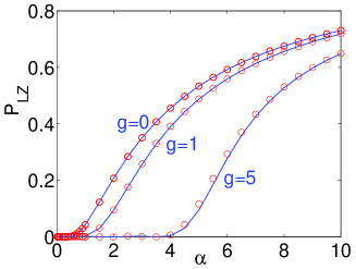
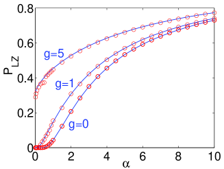
Figure 1: Landau-Zener tunneling probability in the lower level (left) and the upper level (right) for $J=1$ and $g=0,1,5$. Mean-field results $P_{\rm LZ}^{\rm mf}(\alpha)$ are plotted as solid blue lines, many-particle results $P_{\rm LZ}^{\rm mp}(\alpha)$ for $N=50$ particles as red circles.

Within the phase space description, the expectation values of the generalized angular momentum operators (3) are obtained by an integration over the quasi-probability density:

$$\langle\hat{\mathbf{L}}\rangle=(N+2)\int\mathbf{s}(\theta,\phi)Q(\theta,\phi)\sin\theta{\rm d}\theta{\rm d}\phi.$$ (14)

As a direct consequence, we can calculate the reduced single particle density matrix (SPDM), which is defined as

$$\rho=\left(\begin{array}[]{c c}1/2-\langle\hat{L}_{z}\rangle/N&\langle\hat{L}_{x}\rangle/N-{\rm i}\langle\hat{L}_{y}\rangle/N\\ \langle\hat{L}_{x}\rangle/N+{\rm i}\langle\hat{L}_{y}\rangle/N&1/2+\langle\hat{L}_{z}\rangle/N\\ \end{array}\right).$$ (17)

The SPDM is a very useful quantity, since it characterizes the many-body quantum state of the trapped atoms. In particular, the fraction of atoms condensed to a single quantum state (the BEC) is given by the leading eigenvalue of the SPDM [32]. If the the expectation value $\langle\hat{\mathbf{L}}\rangle/N$ lies on the Bloch sphere, i.e. has a magnitude of $1/2$ (as it is always the case in the common single-trajectory mean-field approach), then the two eigenvalues of the SPDM are always $\{0,1\}$ indicating a pure BEC. The phase space representation is not limited to product states. Due to the averaging procedure in equation (14), the expectation value of the Bloch vector is then no longer restricted to the surface, but can lie anywhere inside the Bloch sphere. The phase space approach has been proven to be a very useful tool to go beyond the usual mean-field description [27], especially in the description of dynamical instabilities, where it is clearly not sufficient to take into account only expectation values and to neglect all higher moments. As we show in the following, this approach also resolves the non-commutability of the adiabatic and the semiclassical limit, which therefore must be considered as an artifact of the single-trajectory description.

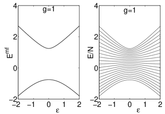
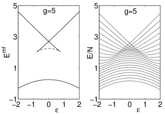
Figure 2: Energy of the mean-field stationary states (18) in comparison to the eigenenergies of the two-mode Bose-Hubbard model (2) in dependence of the offset $\epsilon$ for $J=1$ and $g=1$ (left) and $g=5$ (right) and $N=20$ particles.

3 Nonlinear Landau-Zener tunneling

The nonlinear self-interaction fundamentally alters the dynamics of the system [14, 15, 17] and strongly influences the Landau-Zener transition probability, as can be seen in figure 1. The solid lines show the mean-field Landau-Zener tunneling probability (10) in dependence of the parameter velocity $\alpha$ for different values of the interaction strength $g$. For this calculation we have used the common single-trajectory mean-field approximation. However, there are no visible differences to the phase-space results for the actual parameters. The open circles represent the corresponding many-particle results. In the linear case $g=0$, one recovers the result (1) for the Landau-Zener tunneling probability. For a slow parameter variation, the state can adiabatically follow the instantaneous eigenstates and thus most particles tunnel coherently to the other well. For a faster sweep, this coherent tunneling effect is strongly disturbed such that the Landau-Zener transition probability no longer vanishes. This effect is present in both, the transition probability in the upper and the lower level.

In the nonlinear case, the tunneling probability becomes strongly asymmetric: it increases as $g$ increases in the upper level, while it decreases in the lower level. To understand this effect, it is insightful to consider the total energy of the mean-field system. Figure 2 shows the eigenenergies of the Hamiltonian (2) in comparison to the total energies of the ‘nonlinear eigenstates’, i.e. the stationary states of the mean-field dynamics (7),

$$E^{\rm mf}=\epsilon(|\psi_{2}|^{2}-|\psi_{1}|^{2})-J(\psi_{1}^{*}\psi_{2}+\psi_{2}^{*}\psi_{1})+\frac{g}{2}(|\psi_{1}|^{4}+|\psi_{2}|^{4}).$$ (18)

Compared to the non-interacting case $g=0$, the left-hand side shows that the upper level is sharpended, while the lower level is flatened for small interactions $0<g<2J$. This flattening supresses the tunneling probability from the lower level to the upper level, leading to a decreased Landau-Zener probability in the adiabatic regime. On the other hand, the sharpening of the upper level makes it more difficult to follow the adiabatic eigenstates, which results in a increased Landau-Zener probability for the upper level, as can be seen on the right-hand side of figure 1.

Most remarkably, the tunneling probability in the upper level does not even vanish in the adiabatic limit $\alpha\rightarrow 0$ for $g>2J$, i.e. adiabaticity breaks down in the strongly interacting case.

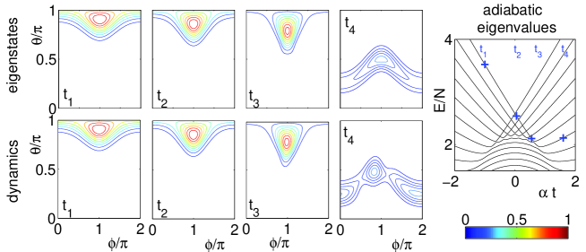
Figure 3: Dynamics of the many-particle Landau-Zener transition for $J=1$, $g=5$, $N=20$ and $\alpha=0.1$. The upper figures show a contour plot of the Husimi distribution of the instantaneous eigenstates marked in the level scheme on the right at times $t_{j}=-10,0.5,5.5,16$. The lower figures show the Husimi distribution of the dynamical quantum state $|\Psi(t)\rangle$ at the same times.

In order to explore the origin of this breakdown of adiabaticity we compare again the eigenstates of the many-particle system to the stationary states of the mean-field system. For $g>2J$ the mean-field eigenenergies show a swallow’s tail structure in the upper level, reflecting the occurrence of a bifurcation of one of the steady states into three new ones, one of them hyperbolically unstable (dashed line) and two elliptically stable (solid lines). The system can adiabatically follow the steady states as long as these are elliptically stable. This is possible only until the end of the swallow’s tail where the elliptic fixed point vanishes in an inverse bifurcation with the hyperbolic fixed point [15, 16]. Then the dynamics becomes unstable and adiabaticity is lost even for very small values of $\alpha$.

The swallow’s tail in the mean-field energy corresponds to a caustic of the many-particle eigenenergy curves in the limit $N\rightarrow\infty$, which are bounded by the mean-field energies from below and above. Within this caustic one finds a series of quasi-degenerate avoided crossings of the many-particle levels. The level splitting at these crossings tends to zero exponentially fast in the mean-field limit $N\rightarrow\infty$ with $g=UN$ fixed [19, 34]. Thus the system will show a complete diabatic time evolution at these quasi-crossings even for very small values of $\alpha$. Outside the swallow’s tail one finds common avoided crossings, where the system evolves adiabatically for small value of $\alpha$.

Note, however, that the breakdown of adiabaticity is only approximate for the many-particle system. It is known that for a symmetric tridiagonal Hamiltonian, such as the one we are considering (2) with $J\neq 0$, the level spacings in the spectrum may be exponentially small but nevertheless always non-zero [33]. Thus adiabaticity can be restored when the parameter velocity $\alpha$ is decreased well below the square of the residual level splitting $\Delta$ [34]:

$$\alpha\stackrel{{\scriptstyle!}}{{\ll}}\Delta^{2}\qquad\mbox{with}\qquad\Delta\propto N\exp(-\eta N),$$ (19)

where $\eta$ is a proportionality constant which depends of the system parameters. However, the adiabaticity condition on the velocity becomes exponentially difficult to fulfill. Thus the breakdown of adiabaticity is also present in the full many-particle system for any realistic set of parameters. The same dynamics is found for attractive nonlinearities, $g<0$, only the roles of the upper and lower level are exchanged.

4 Phase space picture

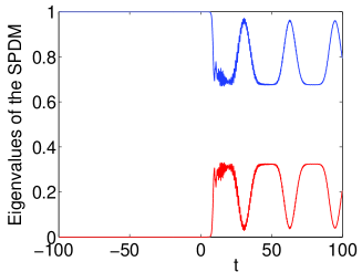
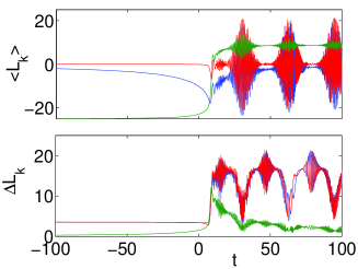
Figure 4: Dynamics of the many-particle Landau-Zener transition for $g=5$, $N=50$ and $\alpha=0.1$. The left figure shows the eigenvalues of the SPDM (17). The expectation values $\langle\hat{L}_{k}\rangle$ and widths $\Delta\hat{L}_{k}$ of the angular momentum operators (3) for $k=x$ (blue), $k=y$ (red) and $k=z$ (green) are plotted on the right-hand side. The onset of the oscillatory dynamics corresponds to the cusp of the swallow-tail structure in the mean-field representation (cf. figure 2).

Further insight into the dynamics of nonlinear Landau-Zener tunneling can be gained within the phase space picture introduced in section 2 and in [26, 27].

According to the remarks in the previous section, the system will undergo a series of diabatic transitions up to the end of the swallow’s tail and evolve adiabatically afterwards. To verify these claims, we compare the actual many-particle quantum state $|\Psi(t)\rangle$ to the instantaneous eigenstate in figure 3 at four points in time during a Landau-Zener passage. To visualize the quantum states, we use the Husimi distribution $Q(\theta,\phi,t)$ as defined in equation (11). The right-hand side of figure 3 illustrates the series of diabatic/adiabatic transitions and the specific instantaneous eigenstates shown in upper panels of the figure. One observes a good agreement between the dynamical state and the instantaneous eigenstates, during the transition as well as afterwards. However, the crossover from diabatic to adiabatic transitions is not absolutely sharp. The final state contains small contributions from other instantaneous eigenstates.

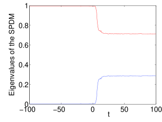
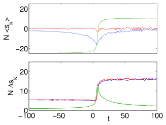
Figure 5: Semiclassical simulation of the many-particle Landau-Zener transition for $J=1$, $g=5$, $N=50$ and $\alpha=0.1$. The left figure shows the eigenvalues of the ensemble approximation for the SPDM $\rho_{kl}=\langle\psi_{k}^{*}\psi_{l}\rangle_{\rm cl}$. The ensemble expectation values $N\langle s_{k}\rangle_{\rm cl}$ and the standard deviation $N\Delta s_{k}$ of the Bloch vector (8) for $k=x$ (blue), $k=y$ (red) and $k=z$ (green) are plotted on the right-hand side.

In order to characterize the many-particle quantum state during the Landau-Zener transition, we have plotted the eigenvalues of the SPDM (17) on the left-hand side of figure 4. One eigenvalue remains equal to unity, while the other one vanishes, indicating a fully coherent state until the crossover from diabatic to adiabatic transitions. Then one observes an oscillation of the SPDM eigenvalues: The contributions of the different many-particle eigenstates de- and rephase periodically giving rise to a beat signal which is genuinely quantum. The oscillation of the coherence is mirrored in the evolution of the uncertainties of the angular momentum operators $\Delta\hat{L}_{x}$ and $\Delta\hat{L}_{y}$ shown on the right-hand side of figure 4. The uncertainties are strongly enhanced when the coherence is (partly) lost. This behaviour can be intuitively explained in terms of the dynamics of the Husimi distribution. The centre of mass of the Husimi function oscillates rapidly in the $\phi$-direction, leading to oscillations of the expectation values $\langle\hat{L}_{x}\rangle$ and $\langle\hat{L}_{y}\rangle$. Furthermore the distribution breathes in the $\phi$-direction at a slower timescale, leading to the oscillations of the width $\Delta\hat{L}_{x}$ and $\Delta\hat{L}_{y}$ and the periodic revivals of the coherence. The oscillations of the expectation values die out at the times when the Husimi function is spread nearly uniformly in the $\phi$-direction, i.e. at the times where the coherence is minimal. In contrast, the Husimi distribution is well localized in the $\theta$-direction for long times and the corresponding uncertainty $\Delta\hat{L}_{z}$ remains small. The population difference $\langle\hat{L}_{z}\rangle$ is thus well described by the simple Bogoliubov mean-field approximation. Many-particle and mean-field results for the Landau-Zener tunneling rate show an excellent agreement (cf. figure 1), because they depend only on the population difference and not on the coherence.

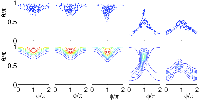
Figure 6: The many-particle Landau-Zener scenario in phase space. The dynamics of an ensemble of 150 classical trajectories (upper panels) is compared to the evolution of the Husimi distribution (lower panels) at times $t=-16,-8,0,8,16$ (from left to right). Parameters are chosen as in figure 3.

The evolution of the coherence and the uncertainties $\Delta\hat{L}_{x}$ and $\Delta\hat{L}_{y}$ certainly goes beyond the Bogoliubov mean-field approximation, but most of the effects can be taken into account by the semi-classical phase space approach introduced in section 2 and in [26, 27]. Figure 6 shows the dynamics of the many-particle Landau-Zener scenario in quantum phase space in comparison to the dynamics of a classical phase space ensemble. The expectation values and variances of the Bloch vector $\hat{\mathbf{L}}$ calculated from such an ensemble simulation are plotted in figure 5. It is observed, that the spreading of the Husimi distribution in the direction of the relative phase $\phi$ and the loss of coherence are well reproduced by the classical ensemble. However, the quantum beat oscillations of the coherence are of course not present in the classical distributions as shown in figure 5. The expectation value and the fluctuations of the classical Bloch vector $\mathbf{s}$ defined in equation (8) show a similar effect. The global dynamics of the angular momentum operator $\hat{\mathbf{L}}$ plotted in figure 4 is well reproduced, whereas all the quantum beats are absent. These are genuine many-particle quantum effects.

The previous results show that the many-particle quantum state after a nonlinear Landau-Zener sweep is far from being a pure BEC. In particular it has been claimed that the final state is strongly number squeezed in comparison to a pure BEC with the same density distribution [42]. The figures 4 and 5 show the evolution of the expectation values and variances of $\hat{\mathbf{L}}$, comparing many-particle results to a phase space approximation. One observes that the number fluctuations $\Delta L^{2}_{z}$ are strongly increased during the sweep, but relax to a smaller value again afterwards. This evolution is well described within the semiclassical phase space picture. A further quantitative analysis of number squeezing during a Landau-Zener sweep is provided in figure 7, comparing exact results (red) to an ensemble simulation (green). For a pure BEC with a given particle density, number fluctuations are given by $\Delta L^{2}_{z,\rm ref}=\langle\hat{n}_{1}\rangle\langle\hat{n}_{2}\rangle/N$. Thus one can define the parameter $\xi_{N}^{2}=\Delta L^{2}_{z}/\Delta L^{2}_{z,\rm ref}$, which measures the suppression of number fluctuations in comparison to a pure BEC. Figure 7 (a) shows the value of $\xi_{N}^{2}$ during a slow Landau-Zener sweep with $\alpha=0.1$. Indeed, $\xi_{N}^{2}$ drops well below one for long times indicating number squeezing. Again, this feature is well reproduced by a phase space simulation (green). The final value of $\xi_{N}^{2}$ after the sweep is shown in Figure 7 (b) as a function of the parameter velocity $\alpha$. Number squeezing with $\xi_{N}^{2}<1$ is observed for small values of $\alpha$ in the regime of the breakdown of adiabaticity, e.g. for large interaction strength, $2J<g$ . The phase space simulation overestimates the variances and thus also $\xi_{N}^{2}$, but gives the correct overall behaviour. For fast sweep, $\xi_{N}^{2}$ tends to one as the state remains approximately coherent.

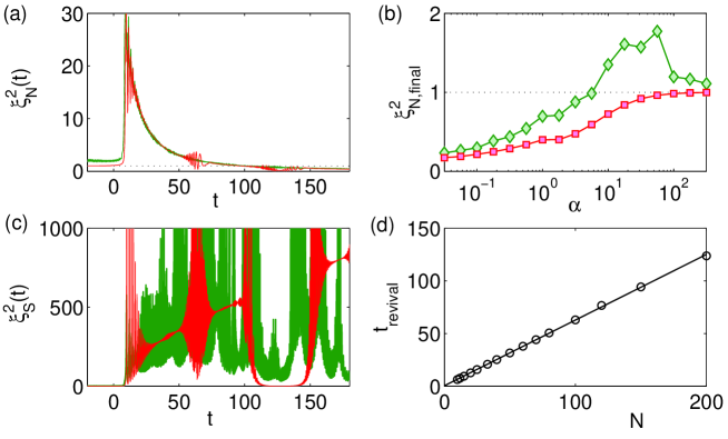
Figure 7: Number squeezing during a Landau-Zener sweep. Many-particle results (red) are compared to an ensemble simulation (green). (a) Evolution of the relative squeezing parameter $\xi_{N}^{2}$ for a slow sweep with $\alpha=0.1$. (b) Final value of $\xi_{N}^{2}$ after the sweep as a function of the parameter velocity $\alpha$. (c) Evolution of the spectroscopic squeezing parameter $\xi_{S}^{2}$ for a slow sweep with $\alpha=0.1$. (d) Dependence of the revival time of the occurrence of a squeezed state on the particle number $N$. The remaining parameters are $J=1$, $g=-5$ and $N=200$ particles.

However, an application of number squeezing in quantum metrology requires a reduction of number fluctuations as well as a large phase coherence. Thus, a quantum state is defined to be spectroscopically squeezed if and only if

$$\xi_{S}^{2}:=N\frac{\Delta\hat{L}_{z}^{2}}{\langle\hat{L}_{x}\rangle^{2}+\langle\hat{L}_{y}\rangle^{2}}<1.$$ (20)

Spectroscopic squeezing indicates multipartite entanglement of the trapped atoms [40, 41]. The evolution of the squeezing parameter $\xi_{S}^{2}$ during a slow Landau-Zener sweep with $\alpha=0.1$ is plotted in figure 7 (c). While the number fluctuations $\Delta\hat{L}_{z}^{2}$ assume a small constant value after the sweep, the phase coherence $\langle\hat{L}_{x}\rangle^{2}+\langle\hat{L}_{y}\rangle^{2}$ strongly oscillates due to the periodic de- and rephasing of the many-particle eigenstates (cf. figure 4). True spin squeezing with $\xi_{S}^{2}<1$ is present only temporarily in the periods of maximum phase coherence. The timescale of the occurence of these minima depends linearly on the particle number $N$, as shown in figure 7 (d). For macroscopic particle numbers it takes very long before the states rephase such that $\xi_{S}^{2}<1$ is observed. Moreover these revivals are extremely sensitive to phase noise. Thus, it is doubtful that for realistic particle numbers Landau-Zener sweeps may be useful to generate squeezed states in a controlled way. Finally we note that the revivals of the phase coherence are not described by the phase space picture. Even small fluctuations in the phase coherence lead to large errors. Therefore the phase space approximation cannot account for the short periods where true spin squeezing $\xi_{S}^{2}<1$ is observed.

Let us finally investigate the global dependence of the Landau-Zener tunneling rate on the interaction strength $g=UN$ in more detail. To this end we calculate the quantum and the classical tunneling rates given by equations (6) and (10), respectively, as well as the eigenvalues of the SPDM (17). We consider an initial state that is localized in the upper level for $t\rightarrow-\infty$ so that adiabaticity breaks down for a repulsive nonlinearity $g>2J$. As discussed above, a change of the sign of the interaction strength $g$ corresponds to an interchange of the two modes. For an attractive nonlinearity, adiabaticity breaks down in the lower level instead. Thus we obtain a global picture of the dynamics either by calculating the tunneling rate in the upper and the lower level for $g>0$, or by calculating the tunneling rate in the upper level alone for $g>0$ and $g<0$. In the following we choose the latter option.

Figure 8 shows the results for $J=1$ and $\alpha=0.1$, where the linear system evolves completely adiabatically. The left-hand side shows the many-particle and mean-field Landau-Zener tunneling probabilities as defined in equation (6) and (10), respectively. The right-hand side shows the eigenvalues of the SPDM (17) for $t\rightarrow+\infty$. Note, however, that the eigenvalues of the SPDM oscillate for $t>0$ as shown in figure 4, indicating a periodic loss and revival of coherence. Figure 8 shows the eigenvalues of the SPDM for large times, omitting the temporal revivals explicitly. As expected, adiabaticity breaks down as soon as $g>2J$ and the Landau-Zener tunneling rate increases with $g$. In the adiabatic regime, one eigenvalue of the SPDM is close to zero, indicating a fully coherent state. Coherence is lost when the adiabaticity breaks down and particles are scattered out of the condensate mode.

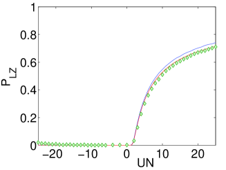
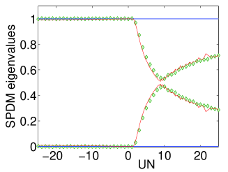
Figure 8: Left panel: Landau-Zener tunneling probability as a function of of the interaction strength $UN$ for a slow parameter variation $\alpha=0.1$ and $J=1$, $N=50$. Right panel: Eigenvalues of the SPDM for $t\rightarrow+\infty$. The exact many-particle results (red line) are compared to a phase space ensemble simulation (green diamonds) and the single-trajectory mean-field results (blue line).

Figure 9 shows the results for a fast sweep $\alpha=10$ for $J=1$. In the linear case, equation (1) predicts a Landau-Zener tunneling rate of $P_{\rm LZ}=0.7304$. Surprisingly, the basic structure of the numerical results is very similar to the adiabatic case shown in figure 8. The curves are shifted, but the general progression remains the same. This is understood as follows. As argued above, an attractive nonlinearity flattens the upper level so that Landau-Zener tunneling is decreased. The current example shows that this effect is so strong that the tunneling process is completely suppressed so that $P_{\rm LZ}\rightarrow 0$ for large negative values of $g$. On the contrary, a repulsive nonlinearity leads to an increase of $P_{\rm LZ}$. The transition between an effectively adiabatic and non-adiabatic dynamics occurs at $g=2J$ for a slow parameter variation $\alpha\rightarrow 0$. For a fast sweep, $P_{\rm LZ}$ is non-zero in the linear case $g=0$. However, a strong attractive nonlinearity can flatten the level so much that adiabaticity is restored again. Thus one can always enforce an adiabatic transition, but the necessary interaction strength $|g|$ increases monotonically with $\alpha$. This behaviour is also reflected in the coherence properties of the final state shown on the right-hand side of figure 8 and 9.

One astonishing feature observed in the figures 8 and 9 is the excellent agreement of the Landau-Zener tunneling rate $P_{\rm LZ}$ and the eigenvalues of the SPDM. Deviations are only found around $g=0$ in figure 9. This can be understood by a loss of the coherence between the two modes for long times, i.e.

$$\langle\hat{a}_{1}^{\dagger}\hat{a}_{2}\rangle\rightarrow 0\qquad\mbox{for}\quad t\rightarrow+\infty,$$ (21)

if we do not take into account for the temporal revivals illustrated in figure 4. This happens either if the atoms are not in a coherent state any longer or if all atoms are localized in one of the modes. In any case we can rewrite the reduced SPDM as

$$\rho(t\rightarrow+\infty) \approx \left(\begin{array}[]{c c}\langle\hat{n}_{1}(t\rightarrow+\infty)\rangle&0\\ 0&\langle\hat{n}_{2}(t\rightarrow+\infty)\rangle\\ \end{array}\right)$$ (24)

$$= \left(\begin{array}[]{c c}1-P_{\rm LZ}&0\\ 0&P_{\rm LZ}\\ \end{array}\right).$$ (27)

So the eigenvalues of the SPDM are directly given by the Landau-Zener tunneling rate if the two modes are not coherent. For strong nonlinearities $g$ this is always the case and so the left- and the right-hand sides of the figures 8 and 9 show an excellent agreement except for a small region around $g=0$ in figure 9. In the non-interacting case ($g=0$) the dynamics of all atoms is identical and the condensate will be fully coherent at all times. Thus the leading eigenvalue of the SPDM is always equal to unity independent of the Landau-Zener tunneling rate, such that the approximation (24) is no longer valid in the non-interacting case.

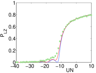
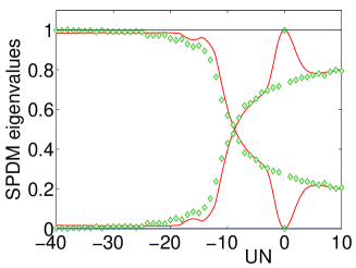
Figure 9: Left panel: Landau-Zener tunneling probability as a function of of the interaction strength $g=UN$ for a fast parameter sweep $\alpha=10$ and $J=1$, $N=50$. Right panel: Eigenvalues of the SPDM for $t\rightarrow+\infty$. The exact many-particle results (red line) are compared to a phase space ensemble simulation (green diamonds) and the single-trajectory mean-field results (blue line).

5 Semiclassical and adiabatic limit

Having discussed various aspects of the mean-field many-particle correspondence in the previous sections, we now investigate the convergence to the mean-field limit quantitatively. The left-hand side of figure 10 compares the mean-field Landau-Zener tunneling probability $P_{\rm LZ}(\alpha)$ (10) to the corresponding many-particle results (6) for different particle numbers and $g=-5$. While the many-particle dynamics usually converges rapidly to the mean-field limit, the occurence of a dynamical instability for $|g|>2J$ leads to a breakdown of adiabaticity for small values of $\alpha$. In this parameter region the convergence to the many-particle limit is logarithmically slow. This is further illustrated in figure 10 on the right-hand side, where the Landau Zener tunneling probability $P_{\rm LZ}^{\rm mp}$ is plotted as a function of the inverse particle number $1/N$.

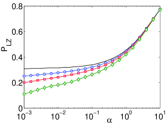
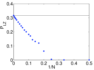
Figure 10: Left panel: Landau-Zener tunneling probability $P_{\rm LZ}$ as a function of $\alpha$ for $g=-5$. Single-trajectory mean-field results (solid black line) are compared to exact many-particle results for $N=10$ (green diamonds), $N=20$ (red squares) and $N=40$ (blue circles) particles. The lines are drawn to guide the eye. Right panel: Slow convergence to the mean-field limit in the adiabatic regime. The Landau-Zener tunneling probability $P_{\rm LZ}$ is plotted as a function of the inverse particle number for $\alpha=0.01$ and $g=-5$. The black line corresponds to the single-trajectory mean-field results which are approached in the limit $1/N\rightarrow 0$.

Another observation that can be drawn from the numerical data presented in figure 10 is that a simple mean-field description gives qualitatively wrong results in the adiabatic limit of small $\alpha$. As already discussed in section2, the many-particle Landau-Zener tunneling probability $P_{\rm LZ}^{\rm mp}(\alpha)$ will always tend to zero for $\alpha\rightarrow 0$ since the level splittings in the many-particle spectrum may become small, but are always non-zero for finite $N$. Its mean-field counterpart $P_{\rm LZ}^{\rm mf}(\alpha)$ , however, is always affected by the appearance of the dynamical instability which destroys adiabaticity also for infinitesimally small values of $\alpha$. Consequently, the Landau-Zener tunneling probability is believed to be non-zero even in this limit. This difference led to the claim that the adiabatic limit $\alpha\rightarrow 0$ and the semiclassical limit $1/N\rightarrow 0$ do not commute [34]. However, this claim is true only for the single-trajectory mean-field description which assumes a pure condensate at all times, which is obviously no longer true in the present case.

As discussed in the previous section, the proper semiclassial limit of the quantum dynamics is a phase space flow rather than a single phase space trajectory. This description is valid also if the classical dynamics is unstable and the many-particle quantum state deviates from a pure condensate. The left-hand side of figure 11 shows the Landau-Zener tunneling probability $P_{\rm LZ}^{\,\rm ens}(\alpha)$ for different particle numbers calculated from the propagation of a semiclassical phase space ensemble as described in section 4. It is observed that the many-particle results (cf. figure 10) can be reproduced to a very good approximation even for small values of $\alpha$. Thus there is no incommutability of the adiabatic and semiclassical limits if the latter is interpreted correctly. Also the slow convergence to the single-trajectory limit is well described by the semiclassical phase space approach. The right-hand side of figure 11 shows $P_{\rm LZ}^{\,\rm ens}$ as a function of the inverse particle number $1/N$ for $\alpha=0.01$ which is well in the adiabatic regime. Significant differences to the many-particle results (cf. figure 10) are observed only for very small particle numbers, $N\apprle 10$.

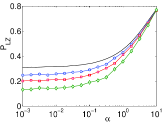
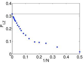
Figure 11: Left panel: Landau-Zener tunneling probability $P_{\rm LZ}^{\,\rm ens}$ as a function of $\alpha$ calculated from a semi-classical ensemble simulation for $g=-5$ and $N=10$ (green diamonds), $N=20$ (red squares) and $N=40$ (blue circles) particles. The lines are drawn to guide the eye. The black line corresponds to the single-trajectory mean-field results which are approached in the limit $1/N\rightarrow 0$. Right panel: The Landau-Zener tunneling probability $P_{\rm LZ}^{\,\rm ens}$ as a function of the inverse particle number calculated from a semi-classical ensemble simulation for $\alpha=0.01$ and $g=-5$.

6 Influence of phase noise

We finally want to approach the question how an interaction with the environment affects the transition from quantum-many body to the classical mean-field dynamics. To this end we consider the Landau-Zener problem subject to phase noise, which is the dominant influence of the environment provided that the two condensate modes are held in sufficiently deep trapping potentials [35, 36]. The many-particle dynamics is then given by the master equation

$$\frac{{\rm d}}{{\rm d}t}\hat{\rho}=-{\rm i}[\hat{H},\hat{\rho}]-\frac{\gamma}{2}\sum_{j=1,2}\left(\hat{n}_{j}^{2}\hat{\rho}+\hat{\rho}\hat{n}_{j}^{2}-2\hat{n}_{j}\hat{\rho}\hat{n}_{j}\right).$$ (28)

The effect of phase noise can be included in a single-trajectory mean-field limit starting from the dynamics of the Bloch vector (8), whose evolution equations are then given by [37, 38, 39]

$$\dot{s}_{x} = -2\epsilon s_{y}-2Us_{y}s_{z}-\gamma s_{x},$$

$$\dot{s}_{y} = 2Js_{z}+2\epsilon s_{x}+2Us_{x}s_{z}-\gamma s_{y},$$

$$\dot{s}_{z} = -2Js_{y}.$$ (29)

Thus, phase noise leads to transversal relaxation degrading the coherences $s_{x}$ and $s_{y}$ of the two condensate modes. Note that the magnitude of the Bloch vector is no longer conserved because of this effect.

The resulting Landau-Zener tunneling probabilities are plotted in figure 12 as a function of $\alpha$ for different values of the noise strength $\gamma$. It is observed that phase noise has an important effect only for small values of $\alpha$, where it drives the system to a completely mixed state with equal population in both wells so that $P_{\rm LZ}=1/2$. On the contrary, almost no consequences are observed for fast parameter sweeps. In this case, the tunneling time during which the atoms are delocalized is so short that phase noise cannot affect the dynamics. The transition to the incoherent regime occurs when the time scale of the noise $\gamma^{-1}$ is smaller than the tunneling time which is roughly given by $\alpha^{-1}$. Therefore the sweep is incoherent such that $P_{\rm LZ}=1/2$ if

$$\alpha\apprle\gamma,$$ (30)

while the interaction strength $g$ has a minor effect only.

Comparing mean-field and many-particle results, significant differences are observed for very small values of $\alpha$ and $g=-5$ in the non-dissipative case $\gamma=0$, which has been discussed in detail above. In addition we note that already a small amount of phase noise is sufficient to remove these differences. For $\alpha\rightarrow 0$ and $\gamma\neq 0$ the mean-field approximation (29) correctly predicts the transition to a completely mixed state with $P_{\rm LZ}=1/2$. Furthermore, significant differences are observed for $g=-5$ and intermediate values of $\alpha$. In this case the many-particle quantum state is no longer a pure BEC but rather strongly number squeezed as discussed above. This state is more easily driven to a completely mixed state by phase noise than a pure BEC, a process which certainly cannnot be described by the simple single-trajectory mean-field approximation.

Finally, these results suggest that Landau-Zener sweeps may actually be used as a probe of decoherence in systems of ultracold atoms (cf. also [4]). A measurement of the transition point to the incoherent regime where $P_{\rm LZ}=1/2$ gives an accurate quantitative estimate of the noise strength $\gamma$ with a fairly simple experiment.

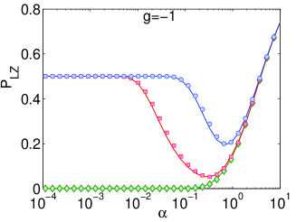
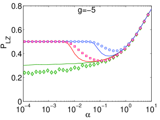
Figure 12: Landau-Zener tunneling probability $P_{\rm LZ}(\alpha)$ in the presence of phase noise for $g=-1$ (left) and $g=-5$ (right). The strength of the phase noise is chosen as $\gamma=0$ (green diamonds), $\gamma=0.01$ (red squares) and $\gamma=0.1$ (blue circles). Mean-field results (solid lines) are compared to many-particle results $N=40$ particles (symbols).

7 Conclusion and Outlook

In the present paper we have presented an analysis of nonlinear Landau-Zener tunneling between two modes in quantum phase space. It was shown that adiabaticity breaks down if the interaction strength $g=UN$ exceeds the critical value $2J$– the Landau-Zener tunneling probability does not vanish even for an extremely slow variation of the system parameter. This phenomenon can be understood by the disappearance of adiabatic eigenstates in an inverse bifurcation in the mean-field approximation. Within the full many-particle description, the breakdown of adiabaticity results from the occurrence of diabatic avoided crossings, where the level separation vanishes exponentially with the number of particles.

The correspondence of the quantum dynamics and the ‘classical’ mean-field approximation has been discussed in detail. The many-particle and the mean-field Landau-Zener tunneling probability show an excellent agreement, because quantum fluctuations of the populations are small. In contrast, there is no fixed phase relation between the two modes, which certainly goes beyond the simple Bogoliubov mean-field theory. An improved classical approximation using phase space ensembles can describe the depletion of the condensate mode and the loss of phase coherence as well as number squeezing $\xi_{N}^{2}$ of the final state. Yet temporal revivals of this coherence are genuine many-particle effects and cannot be described classically. Thus, the spectroscopically relevant squeezing parameter $\xi_{S}^{2}$ is not reproduced by the ensemble simulation. However, the timescale for the occurence of these revivals and accordingly of the spectroscopical squeezing depends linearly on the particle number. For realistic setups, this is way to long compared to decoherence and phase noise rates. Before the sytem reaches the squeezed state, nearly all coherences are already lost.

In the last section, we have studied how the dynamics depends on the number of particles $N$ and compare our results to the discrete Gross-Pitaevskii equation that describes the dynamics in the limit $N\rightarrow\infty$. We show that the contradiction between the mean-field prediction and the exact many-particle transition rate in the adiabatic regime is no longer present in the phase space approach, and must therefore be considered as an artifact of the single-trajectory description. These results demonstrate the power of the phase space approach. However, in order to reproduce true quantum features such as quantum beats semiclassically, a more refined treatment is necessary. Semiclassical coherent state propagators have been studied intensively in single particle quantum mechanics in the limit $\hbar\rightarrow 0$ [43]. An extension to the mean-field limit of quantum many-body system must be based on the $SU(M)$ phase space discussed in the present paper. In this case the particle number $N$ is a number and not an operator and $1/N$ will serve as a proper semiclassical parameter. However, a numerical calculation for realistic particle numbers based on these methods, taking into account all relevant phase information between different trajectories, is as hard as the original quantum problem.

Furthermore, we show that already the presence of a small amount of phase noise is sufficient to introduce enough decoherence to make the system ’classical’, so that the many-particle dynamics is well reproduced with a simple single-trajectory mean-field approach. Finally we have argued that a measurement of the transition to an incoherent Landau-Zener sweep could be used as a sensitive probe of decoherence.

References

- [1] Wernsdorfer W and Sessoli R 1999 Science 284 133
- [2] Child M S 1974 Molecular Collision Theory (Acad. Press, London)
- [3] Spreeuw R J C, Van Druten N J, Beijersbergen M W, Eliel E R and Woerdman J P 1990 Phys. Rev. Lett. 65 2642
- [4] Wubs M, Saito K, Kohler S, Hänggi P and Kayanuma Y 2006 Phys. Rev. Lett. 97 200404
- [5] Kohler S, Hänggi P and Wubs M 2008, In: Path Integrals: New Trends and Perspectives, edited by W. Janke and A. Pelster (World Scientific, Singapore, 2008)
- [6] Cooper K B, Steffen M, McDermott R, Simmonds R W, Oh S, Hite D, Pappas D P and Martinis J M 2004 Phys. Rev. Lett. 93 180401
- [7] Ithier G, Collin E, Joyez P, Vion D, Esteve D, Ankerhold J and Grabert H 2005 Phys. Rev. Lett. 94 057004
- [8] Oliver W D, Yu Y, Lee J C, Berggren K K, Levitov L S and Orlando T P 2005 Science 310 1653
- [9] Saito K, Wubs M, Kohler S, Hanggi P and Kayanuma Y 2006 Europhys. Lett. 76 22
- [10] Landau L D 1932 Phys. Z. Sowjetunion 2 46
- [11] Zener C 1932 Proc. R. Soc. London 137 696
- [12] Majorana E 1932 Nuovo Cimento 9 43
- [13] Stückelberg E C G 1932 Helv. Phys. Acta 5 369
- [14] Wu B and Niu Q 2000 Phys. Rev. A 61 023402
- [15] Zobay O and Garraway B M 2000 Phys. Rev. A 61 033603
- [16] Liu J, Fu L, Ou B Y, Chen S G, Choi D L, Wu B and Niu Q 2002 Phys. Rev. A 66 023404
- [17] Wu B and Niu Q 2003 New J. Phys. 5 104
- [18] Graefe E M, Korsch H J and Witthaut D 2006 Phys. Rev. A 73 013617
- [19] Witthaut D, Graefe E M and Korsch H J 2006 Phys. Rev. A 73 063609
- [20] Breid B M, Witthaut D and Korsch H J 2007 New J. Phys. 9 62
- [21] Jona-Lasinio M, Morsch O, Cristiani M, Malossi N, Müller J H, Courtade E, Anderlini M and Arimondo E 2003 Phys. Rev. Lett. 91 230406
- [22] Fallani L, Sarlo L D, Lye J E, Modugno M, Sears R, Fort C and Inguscio M 2004 Phys. Rev. Lett. 93 140406
- [23] Sias C, Zenesini A, Lignier H, Wimberger S, Ciampini D, Morsch O, and Arimondo E 2007 Phys. Rev. Lett. 98 120403
- [24] Salger T, Geckeler C, Kling S and Weitz M 2007 Phys. Rev. Lett. 99190405
- [25] Zenesini A, Lignier H, Tayebirad G, Radogostowocz J, Ciampini D, Mannella R, Wimberger S, Morsch O and Arimono E 2009 Phys. Rev. Lett. 103 090403
- [26] Trimborn F, Witthaut D and Korsch H J 2008 Phys. Rev. A 77 043631
- [27] Trimborn F, Witthaut D and Korsch H J 2008 Phys. Rev. A 79 2009
- [28] Albiez M, Gati R, Fölling J, Hunsmann S, Cristiani M and Oberthaler M K 2005 Phys. Rev. Lett. 95 010402
- [29] Schumm T, Hofferberth S, Andersson L M, Wildermuth S, Groth S, Bar-Joseph I, Schmiedmayer J and Krüger 2005 Nature Physics 1, 57
- [30] Milburn G J, Corney J, Wright E M and Walls D F 1997 Phys. Rev. A 55 4318
- [31] Smerzi A, Fantoni A, Giovanazzi S and Shenoy S R 1997 Phys. Rev. Lett. 79 4950
- [32] Leggett A J 2001 Rev. Mod. Phys. 73 307
- [33] Wilkinson J H 1965 The Algebraic Eigenvalue Problem (Oxford: Oxford University Press)
- [34] Wu B and Liu J 2006 Phys. Rev. Lett. 96 020405
- [35] Anglin J R 1997 Phys. Rev. Lett. 79 6
- [36] Ruostekoski J and Walls D F 1998 Phys. Rev. A 58 R50
- [37] Trimborn F, Witthaut D and Wimberger S 2008 J. Phys. B: At. Mol. Opt. Phys. 41 171001
- [38] Witthaut D, Trimborn F and Wimberger S 2008 Phys. Rev. Lett. 101 200402
- [39] Witthaut D, Trimborn F and Wimberger S 2009 Phys. Rev. A 79 033621
- [40] Sørensen A, Duan L M, Cirac J I and Zoller, P 2001 Nature 409 63
- [41] Estève J, Gross C, Weller A, Giovanazzi S and Oberthaler M K 2008, Nature 455 1216
- [42] Smith-Mannschott K, Chuchem M, Hiller M, Kottos T and Cohen D 2009 Phys. Rev. Lett. 102 230401
- [43] Baranger M, de Aguiar M A M, Keck F, Korsch H J and Schellhaaß B 2001 J. Phys. A: Math. Gen. 34 7227