Understanding micro-image configurations
in quasar microlensing

Abstract

The micro-arcsecond scale structure of the seemingly point-like images in lensed quasars, though unobservable, is nevertheless much studied theoretically, because it affects the observable (or macro) brightness, and through that provides clues to substructure in both source and lens. A curious feature is that, while an observable macro-image is made up of a very large number of micro-images, the macro flux is dominated by a few micro-images. Micro minima play a key role, and the well-known broad distribution of macro magnification can be decomposed into narrower distributions with $0,1,2,3\ldots$ micro minima. This paper shows how the dominant micro-images exist alongside the others, using the ideas of Fermat’s principle and arrival-time surfaces, alongside simulations.

1 Introduction

In multiply-imaged lensed quasars, each observable “macro” image is composed of many unresolved “micro” images, due to stellar-scale substructure in the lensing galaxy or cluster. The micro-images can vary in response to even the tiny proper motions of stars or galaxies at cosmological distances, causing occasional rapid changes in the observed macro flux.

Much theoretical and numerical work has been done on quasar microlensing, since the original prediction of Chang & Refsdal (1979). The most common strategy, introduced originally by Young (1981) is ray-tracing: one sets up a random star field with mean density and external shear according to some macro model of the lens, and traces rays backwards to the source plane to compute a macro magnification pattern. Recent examples include random motions of stars, with a view of estimating the properties of the microlensing stars and the accretion disk of the quasar source (e.g., Poindexter & Kochanek, 2010b, a). Micro-images do not appear explicitly in this technique. A contrasting approach is to find all the micro-images due to a random star field and add up their fluxes. Paczyński (1986) was the first to do so, and emphasized the large number of micro-images. Subsequent work produced some elegant image-finding algorithms (Witt, 1993; Lewis et al., 1993) and further insight into the nature of micro-images. A recent evaluation of microlensing computational techniques can be found in Bate et al. (2010).

Yet the macro flux appears to be dominated by a few images. Nityananda & Ostriker (1984) argued, theoretically from the statistical properties of a random star field in an external lensing shear, that the formation and merging of a single pair of macro-images would cause a sharp change in the macro flux. Numerical studies of simulated star fields by Rauch et al. (1992) verified this behaviour. Schechter & Wambsganss (2002) considered this further, emphasizing that macro minima and saddles behave differently and supplying a toy model for understanding the difference. Granot et al. (2003) showed that the number of micro minima is well approximated by a Poisson distribution with mean proportional to the macro magnification.

Such considerations lead to the questions: how do the dominant micro images co-exist alongside the many more numerous faint micro-images? And what are the consequences for the brightness of the macro-images? In this paper we attempt to answer these questions, by considering an aspect that has previously not received much attention in the context of quasar microlensing: the geometry of the arrival-time surface.

2 Image configurations

The usefulness of the arrival-time surface is that images, be they of the macro or micro variety, form at its local extrema: minima, maxima (positive-parity images), and saddle points (negative parity). Of all the arrival time contours, the skeletal ones are those that are self-intersecting and hence correspond to saddle points (Blandford & Narayan, 1986). Positive parity images form inside loops created by self-intersecting contours. Saddle-point contours are helpful in understanding the macro-image configuration of lensed quasars (e.g., Saha & Williams, 2003) and have also been useful for studying unusual macro systems (see figures in Rusin et al., 2001; Keeton & Winn, 2003). As we will show, they are also useful for understanding micro-image configurations.

When the matter distribution is continuous, a macrolens generates macro-images whose macro magnification is

$$\bar{M}^{-1}=(1-\bar{\kappa})^{2}-\bar{\gamma}^{2},$$ (1)

where $\bar{\kappa}$ and $\bar{\gamma}$ are the local value of the convergence and shear respectively. The arrival time has the form

$$\textstyle\tau(x,y)=\frac{1}{2}(1-\bar{\kappa}-\bar{\gamma})x^{2}+\frac{1}{2}(1-\bar{\kappa}+\bar{\gamma})y^{2}$$ (2)

Now suppose the continuous matter is broken up into many point-like lenses, keeping the macro convergence of this random star field the same as before, $\bar{\kappa}$. In other words, the Einstein rings of individual stars cover $\bar{\kappa}$ of the area. The constant external shear $\bar{\gamma}$, is the same as before, and the macro magnification has not changed, however, at a random point in the star field, there is no $\kappa$ but there is a varying $\gamma$ from the combined effect of the star field and the external shear. Hence locally, the micro magnification will be

$$M^{-1}=1-\gamma^{2}$$ (3)

The arrival time now takes the form

$$\textstyle\tau(x,y)=\frac{1}{2}(1-\bar{\gamma})x^{2}+\frac{1}{2}(1+\bar{\gamma})y^{2}-\sum_{i}\theta_{i}^{2}\ln\left|{\bf x}-{\bf x}_{i}\right|$$ (4)

where $\theta_{i}$ is the Einstein radius of the $i$-th star. The sum over logarithmic terms indicates that the arrival time surface has acquired a new local maximum at each star, though these will have zero magnification. Many new saddle-point contours also appear, leading to additional local saddle points, as well as occasional minima. All these are new micro-images. At first glance, the arrival time surfaces can look rather complicated, but we will now show that they can be interpreted by decomposing them into simple building blocks, disregarding unimportant components and highlighting the important ones, i.e., those that contain the brighter images.

The decomposition of arrival-time surfaces is best explained graphically. This is done in Figures 1 and 2, which illustrate cases of even and odd parity respectively.

In Figure 1 the top left panel displays a macro maximum. The “tree-rings” plot in that panel is centred on the macro maximum, and contains 30 randomly placed star lenses. Micro-images were found by using a recursive grid search. The curves are the saddle-point contours, that is, those contours of the arrival time (4) which pass through a saddle-point. The micro-images are marked by filled circles according to the micro magnification. In most cases the filled circles are vanishingly small, since most micro-images are very demagnified. Nevertheless, it is easy so see where the micro-images are: crossings of the contours correspond to saddle points, while each little loop encloses a maximum. Each star naturally has a micro maximum at the star position, and most have a micro saddle in the direction of the center. This maximum/saddle micro-image configuration is dictated by the macro shape of the arrival time, which is sloping away from the center. Because the micro saddles have to form between the center and micro maxima, the saddle-point contours have loops pointing outwards. The apparent complexity of this plot should not distract from its basic simplicity: it can be decomposed into many individual loops, as illustrated by the accompanying sketch. Though we have not put points at the locations of micro maxima, they do exist inside each small loop. Note that there are no micro minima in this plot. Given a typical random distribution of stars it would be rather difficult to form a local well close to the hill-top, so micro minima are hardly ever found near macro maxima. (For an example of a microlensed macro maximum, see Dobler et al., 2007)

The other three panels in Figure 1 show macro minima. As before, a star-lens forms a micro maximum, but because the whole configuration is in a well rather than a hill, the resulting micro saddle is in the direction away from the macro minimum. Hence the saddle-point contours have their loops pointing towards the macro minimum, as shown in the accompanying sketch.

Having analyzed the simplest micro-structure of a macro minimum, we can now proceed to more involved cases. In the bottom left panel of Figure 1 we show that a single macro minimum can be split into two with the help of a few star-lenses, which in this case happen to form a partial ridge running vertically in the plot. In terms of saddle-point contours, a new lemniscate, completely embedded in the macro minimum, appears. The sketch above emphasizes that the basic topology is that of a quad, with one or more limaçons surrounding the newly formed lemniscate.

The sequence of three panels of Figure 1, upper right, lower left, and lower right, is primarily a sequence of nested embedding of lemniscates within existing minima, and the accompanying creation of additional micro minima. The lower right panel is the latest step in that sequence, where the right micro minimum hosts a lemniscate; the sketch above highlights the basic topology. This sequence can be extended. Since a minimum necessarily has $M>1$, all micro minima contribute significant flux. The total flux tends to increase with the number of micro minima. Interestingly, the micro saddles adjacent to the micro minima also tend to be non-trivial in terms of flux.

In Figure 2 we show image configurations formed around macro saddles. As before, the original macro-image would have formed at the center of the frame. The upper left panel shows a typical configuration with no micro minima. Star-lenses add numerous saddle-point loops enclosing micro maxima, and adding micro saddles at contour intersections, but these are typically faint. The sketch above it has two configurations; the one on the left is typical; the one on the right can replace the single point saddle-point contour self-intersection. Being symmetric, the configuration in the second sketch is not stable, and hence in practice only approximations to it are seen. A micro minimum can appear near a macro saddle, as shown in the upper right panel. That local well is possible to form because to the upper left and lower left of it the macro-topology has existing “walls”, so just one or two stars to the right are needed to make a local well. The sketch above it also illustrates how a more symmetric version of a typical configuration can create two additional micro saddles.

The lower panels of the same Figure are simple, but common modifications; the left panel shows that similar lemniscate loops can be added on either side of the macro saddle, and the right panel shows that multiple, nested lemniscates can be added on the same side. Again, we see that the micro minima are most important for the flux, with the adjacent micro saddles also contributing significantly.

We remark that the idealized versions of our lower left panel of Figure 1 and the upper left panel of Figure 2 are equivalent to the examples of macro minima and macro saddles that Schechter & Wambsganss (2002) use to explain demagnification of saddles.

The above discussion can be summarized as follows.

• The bright, and hence important images are the micro minima, and their adjacent micro saddles.

• Each star-lens generates a micro maximum and a nearby micro saddle. Generating a micro minimum, however, requires special conditions: a coalition of stars in the proximity of the macro extremum. This is why micro minima are rare; usually just a handful among hundreds of micro-images.

• Nested saddle-point structure arises naturally. One can imagine that if a hierarchy of lens masses is present, i.e., if the mass function is broad, then saddle-point contours and images of lower mass, smaller Einstein radius lenses can be nested within larger ones. This lends another view of the bimodal lens mass model of Schechter et al. (2004).

So far we have put all the mass into stars, which average to $\bar{\kappa}$. However there is no loss of generality with respect to a smoothly-distributed mass component $\kappa_{c}$, as the microlensing effect of the latter can be accounted for by the simple transformation

$$\bar{\kappa}\rightarrow\frac{\bar{\kappa}}{1-\kappa_{c}}\qquad\bar{\gamma}\rightarrow\frac{\bar{\gamma}}{1-\kappa_{c}}$$ (5)

(see e.g., Equation 20 in Paczyński, 1986). Such a transformation multiplies all magnifications by the constant $\left(1-\kappa_{c}\right)^{2}$, and is in fact equivalent (cf. Saha, 2000) to the well-known mass-sheet degeneracy in macrolensing.

Some applications of micro- and milli-lensing call for extended perturbers. Extended lenses can be mimicked to some extent by softening the point lenses, which leaves the basic picture intact, and only moves micro maxima out from under the stars. But we do not attempt general extended lenses in this paper.

3 Macro magnification

The most important observable is the macro magnification. As we saw in the previous section, the brightest images tend to be micro minima, which suggests that the macro magnification will depend primarily on the number of micro mimima. The key role of micro minima has been noted in previous work (Rauch et al., 1992; Schechter & Wambsganss, 2002) but the arrival-time arguments of this paper make it evident.

To quantify our results in terms of the magnification probability distribution we simulated $10^{4}$ realizations of each of the macro minimum and macro saddle cases, with $\bar{M}=\pm 5$ and $\bar{\kappa}=0.5$ (which implies $\bar{\gamma}=0.22$ and $0.67$ respectively). Micro-images were searched for within a square centred on the macro-image position and containing 300 stars randomly distributed. In each realization, of order 300 micro saddles and up to 4 were minima were found.

The small number of minima suggested grouping the realizations according to the number of minima. Figure 3 shows magnification distributions decomposed in this way, with the left and right panel showing macro minima and macro saddles respectively. Similar decompositions appear in Figure 5 of Rauch et al. (1992) and Figure 4 of Granot et al. (2003). It is interesting that all the sub-distributions representing cases with at least one micro minimum have similar shapes, with a steep dropoff on the left and a heavy tail on the right. The case of zero micro minima (thick red histogram in the right panel) is more symmetric.

The sub-distributions overlap, but not to the degree that the individual peaks smear out completely. The total distributions are shown as the solid histograms in Figure 4. As a check we compare these to the magnification distributions obtained with ray-tracing, using a tree code. The ray-tracing algorithm does not find individual images, hence it does not separate out cases according to the number of micro minima. However, the random shear field, Equation 4, is statistically approximated much better, because large buffer region of rays and stars, with up to $10^{5}$ stars outside the main microlensing frame is used, to eliminate edge effects. The two distributions in each panel agree well at macro magnification values below $\bar{M}$ but differ at high magnification. The disagreement at high magnification is expected because the image-finding simulation assumes a point source and hence has an very-high magnification tail not present in the ray-tracing code, which uses a more realistic finite source. The effect of source sizes is an interesting topic, leading for instance to chromatic microlensing due to colour gradients in the source (see e.g., Anguita et al., 2008; Eigenbrod et al., 2008) but we do not investigate it in this paper.

4 Discussion

This paper tries to provide some new insight into micro-image configurations and the magnification distribution arising from it. We find that, despite the large number of micro-images and the complexity of the pattern of images, the micro-image configurations can be understood in terms of the arrival-time surface, as illustrated in Figures 1 and 2. The arrival-time contours in these figures have a very complicated structure reminiscent of tree-rings, but can be seen to be made up much simpler building blocks in the accompanying sketches.

The image configurations are naturally classified according to the number of micro minima, which is almost always small ($1,2,3,4\ldots$ if the macro-image is a minimum, $0,1,2,3\ldots$ if the macro-image is a saddle point). Stars cannot generate micro minima on their own, they do so in conjunction with macro shear. The macro flux is strongly correlated with the number of micro minima. The well-known broad distribution of macro fluxes can be broken down into narrow distributions with different numbers of micro minima, as is displayed in Figure 3. The main difference between the flux distribution for macro minima and macro saddles is that the latter has a sub-distribution with zero micro minima, which is highly demagnified. At least in the cases where microlensing (as opposed to lensing by extended substructure where perturbers contribute $\kappa$ as well) is important, this difference naturally explains the frequent observational occurrence of minimum/saddle image pairs with the latter anomalously faint.

Could the magnification distributions be understood by analytical or partly analytical means? This seems plausible, using the theory of random shear introduced by Nityananda & Ostriker (1984). The probability distribution of the shear due to a random distribution of point masses is (Schneider, 1987b)

$$P(\gamma_{*})=\bar{\kappa}\,\gamma_{*}\left(\bar{\kappa}^{2}+\gamma_{*}^{2}\right)^{-3/2}$$ (6)

The total shear $\gamma$ is the resultant of $\gamma_{*}$ and the macro shear $\bar{\gamma}$ (see also Equation A17 in Nityananda & Ostriker, 1984). The formula (6) has led to several interesting analytical results. Starting from (6), and incorporating macro shear separately, Schneider (1987a) derived the probability distribution of high magnification events, and showed it to be independent of the stellar mass function. Also with the help of (6), Wambsganss et al. (1992) derived an expression for the mean number of macro minima for the case of no macro-shear, which Granot et al. (2003) later generalized to include nonzero $\bar{\gamma}$. But perhaps most relevant is the derivation by Lee & Spergel (1990) of an analytical expression for the magnification probability distribution, assuming a single micro-image dominates, and there is no macro shear. It would be very interesting if their result could be generalized to include external shear, and allow for several micro-images.

5 Acknowledgements

LLRW thanks the Pauli Center for Theoretical Studies, run jointly by the University of Zürich and ETH Zürich, for sabbatical support. The authors also thank the referee for many useful comments.

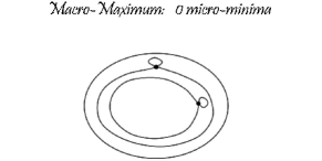
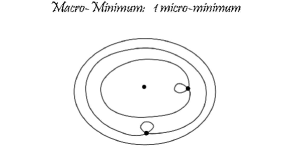
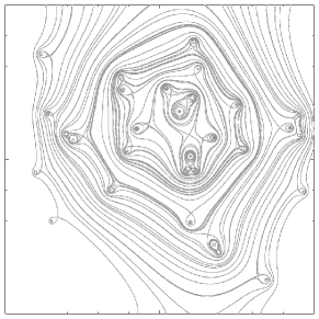
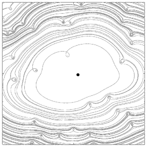
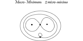
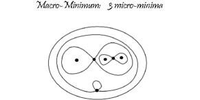
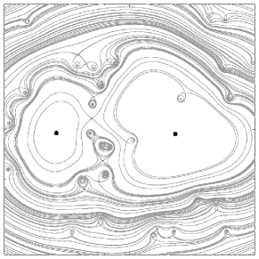
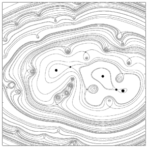
Figure 1: Saddle-point contours for even macro parity. Shown here are examples from simulations showing 0,1,2 and 3 micro minima. The accompanying sketches give the qualitative features of the arrival-time surface. Filled circles denote micro-images with significant flux. The area of these circles is proportional to the flux.

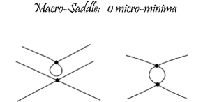
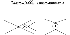
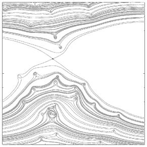
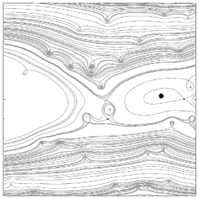
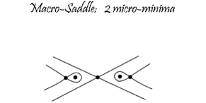
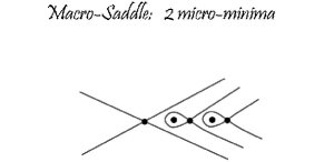
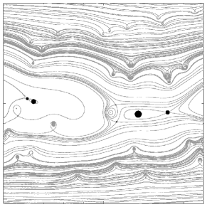
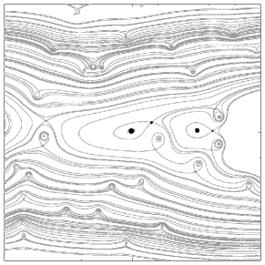
Figure 2: Saddle-point contours for odd macro parity. Shown here are examples from simulations showing 0,1, and 2 micro minima. As in Figure 1, the accompanying sketches give the qualitative features of the arrival-time surface, while filled circles denote micro-images with significant flux, the area of these being proportional to the flux.

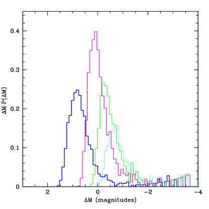
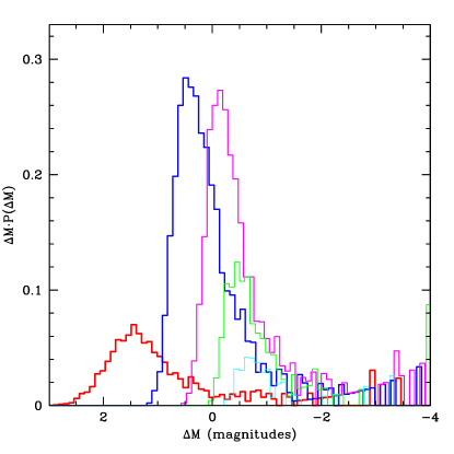
Figure 3: Magnification histograms for a macro minimum (left) and macro saddle (right). The average magnification and surface mass density are the same for both, $\bar{M}=\pm 5$ and $\bar{\kappa}=0.5$, which implies $\bar{\gamma}=0.22$ and $0.67$, for the two panels. The five distributions for the macro minimum show how the total magnification histogram is broken down according to the number of micro minima (from left to right): 1 (thickest, blue line), 2 (magenta), 3 (green) and 4 (thinnest, cyan line). The macro saddle (right panel) is broken down in to six distributions: in addition to the five already mentioned, there is a still thicker (red) line representing macro sadxdles with 0 micro minima. $\Delta M$ is total magnification (or flux) relative to the macro value. Note that the vertical axis is $\Delta M\,P(\Delta M)$, rather than $P(\Delta M)$, in order to make equal areas correspond to equal probabilities, since the horizontal axis is logarithmic. Vertical normalization is arbitrary.

Figure 4: Similar to Figure 3, but here the solid line is the total of the sub-distributions presented in the corresponding panels of Figure 3, while the dashed line was obtained from a ray tracing microlensing simulation.

References

- Anguita et al. (2008) Anguita T., Schmidt R. W., Turner E. L., Wambsganss J., Webster R. L., Loomis K. A., Long D., McMillan R., 2008, A&A, 480, 327
- Bate et al. (2010) Bate N. F., Fluke C. J., Barsdell B. R., Garsden H., Lewis G. F., 2010, ArXiv 1005.5198
- Blandford & Narayan (1986) Blandford R., Narayan R., 1986, ApJ, 310, 568
- Chang & Refsdal (1979) Chang K., Refsdal S., 1979, Nature, 282, 561
- Dobler et al. (2007) Dobler G., Keeton C. R., Wambsganss J., 2007, MNRAS, 377, 977
- Eigenbrod et al. (2008) Eigenbrod A., Courbin F., Meylan G., Agol E., Anguita T., Schmidt R. W., Wambsganss J., 2008, A&A, 490, 933
- Granot et al. (2003) Granot J., Schechter P. L., Wambsganss J., 2003, ApJ, 583, 575
- Keeton & Winn (2003) Keeton C. R., Winn J. N., 2003, ApJ, 590, 39
- Lee & Spergel (1990) Lee M. H., Spergel D. N., 1990, ApJ, 357, 23
- Lewis et al. (1993) Lewis G. F., Miralda-Escude J., Richardson D. C., Wambsganss J., 1993, MNRAS, 261, 647
- Nityananda & Ostriker (1984) Nityananda R., Ostriker J. P., 1984, Journal of Astrophysics and Astronomy, 5, 235
- Paczyński (1986) Paczyński B., 1986, ApJ, 301, 503
- Poindexter & Kochanek (2010a) Poindexter S., Kochanek C. S., 2010a, ApJ, 712, 668
- Poindexter & Kochanek (2010b) Poindexter S., Kochanek C. S., 2010b, ApJ, 712, 658
- Rauch et al. (1992) Rauch K. P., Mao S., Wambsganss J., Paczyński B., 1992, ApJ, 386, 30
- Rusin et al. (2001) Rusin D., Kochanek C. S., Norbury M., Falco E. E., Impey C. D., Lehár J., McLeod B. A., Rix H., Keeton C. R., Muñoz J. A., Peng C. Y., 2001, ApJ, 557, 594
- Saha (2000) Saha P., 2000, AJ, 120, 1654
- Saha & Williams (2003) Saha P., Williams L. L. R., 2003, AJ, 125, 2769
- Schechter & Wambsganss (2002) Schechter P. L., Wambsganss J., 2002, ApJ, 580, 685
- Schechter et al. (2004) Schechter P. L., Wambsganss J., Lewis G. F., 2004, ApJ, 613, 77
- Schneider (1987a) Schneider P., 1987a, ApJ, 319, 9
- Schneider (1987b) Schneider P., 1987b, A&A, 179, 80
- Wambsganss et al. (1992) Wambsganss J., Witt H. J., Schneider P., 1992, A&A, 258, 591
- Witt (1993) Witt H. J., 1993, ApJ, 403, 530
- Young (1981) Young P., 1981, ApJ, 244, 756