How to Extract the Geometry and Topology from Very Large 3D Segmentations

Abstract

Segmentation is often an essential intermediate step in image analysis. A volume segmentation characterizes the underlying volume image in terms of geometric information–segments, faces between segments, curves in which several faces meet–as well as a topology on these objects. Existing algorithms encode this information in designated data structures, but require that these data structures fit entirely in Random Access Memory (RAM). Today, 3D images with several billion voxels are acquired, e.g. in structural neurobiology. Since these large volumes can no longer be processed with existing methods, we present a new algorithm which performs geometry and topology extraction with a runtime linear in the number of voxels and log-linear in the number of faces and curves. The parallelizable algorithm proceeds in a block-wise fashion and constructs a consistent representation of the entire volume image on the hard drive, making the structure of very large volume segmentations accessible to image analysis. The parallelized “CGP” C++ source code, free command line tools and MATLAB mex files are avilable from http://hci.iwr.uni-heidelberg.de/software.php.

1 Introduction

Segmentations of volume images partition the volume into different connected components: segments, faces between segments, curves in which several faces meet, as well as the points between these curves, (Fig. 1). The geometry and topology of these components are essential in many analyses. In order to compute features that describe this geometry and topology, a data structure is needed that provides fast access to all components and their adjacency. Volume segmentations are usually stored simply as volume labelings, i.e. as 3-dimensional arrays in which each entry is a label that uniquely identifies the segment to which the voxel belongs. This form of storage does not represent geometry and topology explicitly. Instead, faces between segments and the curves between these faces are encoded only implicitly, as adjacent voxels whose segment labels differ. All that can be obtained from an array in constant computation time is the segment label at a given voxel. Neither is the set of voxels that belong to the same segment readily available, nor are the faces between adjacent segments or the curves in which several of these faces meet. It is not stored explicitly which segments are adjacent, separated by which faces, and in which curves adjacent faces meet.

The new algorithm presented in this article takes a volume labeling as input and extracts the geometry and topology of all components in a block-wise fashion, in a runtime that is linear in the number of voxels and log-linear in the number of faces and curves. Blocks of the volume labeling can be processed either sequentially, on a single computer that might have only a few hundred megabytes of RAM, or in parallel, on several computers, which facilitates geometry and topology extraction from datasets that consist of more than $10^{9}$ voxels. In both cases, a consistent representation of the entire volume segmentation is constructed on the hard drive, in a data structure from which all connected components and their adjacency can be obtained in constant computation time. The new algorithm makes the geometry and topology of large volume segmentations accessible to image analysis. Its parallelized C++ source code, free command line tools and MATLAB mex files are provided.

This article is organized as follows: Related work is discussed in Section 2. In Section 3, the data structure that captures the geometry and topology of a volume segmentation is introduced. The algorithm for its construction is defined in Section 4 and extended in Section 5 to work with limited RAM and in parallel. The correctness of the algorithm is proved and its complexity analyzed. Section 6 describes the efficient storage of the data structure on the hard drive, and Section 7 concludes the article.

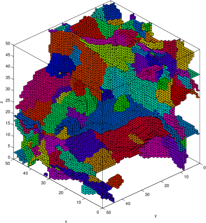
Figure 1: A volume segmentation consists of segments, faces between adjacent segments (left), the curves in which several of these faces meet, as well as the points between these curves (right).

2 Related Work

The first explicit representation of all components of an image segmentation was proposed by Brice and Fennema [1]; it encodes segments as sets of pixels, curves between segments as sets of inter-pixel edges, and the end points of these curves as pixel corners. Naive attempts to represent the different components of a segmentation all as sets of pixels on the pixel grid of the underlying image are topologically inconsistent, as was shown in [2] and proven generally and rigorously in [3, 4]. To overcome this inconsistency, Khalimsky [5] introduced the topological grid whose points correspond to pixels, inter-pixel edges, and pixel corners. The concept of a 3-dimensional topological grid is depicted in Fig. 2.

Data structures that store, for each component of a segmentation, all points on the topological grid that constitute this component were proposed and implemented by [6] for image segmentations and envisioned by [7] for volume image segmentations. However, a storage concept that is suitable for large volume segmentations has so far been missing.

Along with representations of the geometry of segmentations, i.e. their components, at least three different structures have been used to encode the neighborhood system on these objects: Region Adjacency Graphs (RAGs) [2] encode the adjacency of segments. RAGs do not capture the topology of a segmentation completely because several disconnected faces that separate the same two segments correspond to the same edge in the RAG. Kropatsch [8] introduces multiple edges and self-loops in the RAG which results in a multi-graph whose dual graph represents faces as vertices and the adjacency of faces as edges. This concept can be implemented as a data structure. However, both the graph and its dual have to be stored and maintained which is algorithmically challenging.

Combinatorial maps were introduced in image analysis in [9] and are used as data structures, e.g. in [6] as well as in some algorithms of the Computational Geometry Algorithms Library (CGAL). The extension of combinatorial maps to higher dimensions is involved but possible [10, 11] and has facilitated the development of the 3-dimensional topological map [12, 13]. This map captures not only the topology of a segmentation but also its embedding into the segmented space, i.e. containment relations and orders of objects [10, 7]. It is therefore more expensive to construct and manipulate than a data structure that encodes only the topology.

A simple structure that encodes only the topology is a finite cellular complex, cf. [14, 15] also known as a cell complex or CW-complex [16] where CW stands for the two axioms closure-finiteness and weak topology, cf. [15]. Cellular complexes were first used in image processing in [3, 4]. Their generalization to 3D is simple and intuitive.

The main focus of previous efforts to extract and encode the geometry and topology of segmentations has not been on large volume segmentations but on the efficient processing of the merging and splitting of segments. These operations are required within the context of inter-active segmentation. In [17, 7], representations of the geometry and topology are constructed incrementally, using random access to already constructed parts of the data structure. In order for these algorithms to work efficiently, the underlying data structures need to be kept entirely in RAM. To extract the geometry and topology of a volume segmentation of $2,000^{3}$ voxels, $2,000^{3}\cdot 2^{3}\cdot 4$ bytes $\approx 238$ GB of RAM are required for the labeling of the topological grid, an amount that is not available on present day desktop computers. Beyond $3,500^{3}$ voxels, even the $1$ TB of RAM of a large server are insufficient. The method presented in this article overcomes this limitation by means of block-wise processing. It makes geometry and topology extraction from large volume segmentations possible.

Figure 2: A topological grid $T$ is used to represent the geometry of a volume segmentation explicitly. Its elements are called cells. A cell $(t_{1},t_{2},t_{3})\in T$ with $j$ odd entries is called a $j$-cell. 3-cells, 2-cells, 1-cells, and 0-cells respectively represent voxels (blue), faces between voxels (green), lines between faces (red), and points between lines (purple).

3 From Voxels to Geometry and Topology

The starting point for geometry and topology extraction is a volume image on a voxel grid $G=\{1,\ldots,n_{1}\}\times\{1,\ldots,n_{2}\}\times\{1,\ldots,n_{3}\}$ whose extent in each of the three dimensions is given by $n_{1},n_{2},n_{3}\in\mathbb{N}$. Two voxels $v,w\in G$ are said to be connected if $\sum_{j=1}^{3}{|v_{j}-w_{j}|}=1$. Each voxel is thus connected to 6 other voxels unless it is at the boundary of the grid. For every voxel, the connected voxels are called its 6-neighbors. A set of voxels $U\subseteq G$ is called connected if and only if any two distinct voxels $v,w\in U$ are linked by a path in $U$, i.e. by a sequence of voxels in $U$ that starts with $v$ and ends with $w$, in which each voxel is connected to its predecessor.

A volume segmentation partitions the voxel grid $G$ into connected components called segments. A volume labeling

$$\sigma:G\rightarrow\mathbb{N}$$ (1)

assigns to each voxel a label that identifies the segment to which the voxel belongs. Since each voxel belongs to a segment, the faces between segments, the curves between these faces and the points between these curves (Fig. 1) cannot be represented on the voxel grid. The structure that is used for this purpose is a topological grid,

$$T=\{1,\ldots,2n_{1}-1\}\times\{1,\ldots,2n_{2}-1\}\times\{1,\ldots,2n_{3}-1\}\enspace.$$ (2)

This grid has about eight times the size of the voxel grid. Its elements are called cells. Cells with $j$ odd entries are called $j$-cells, cf. Fig. 2.

Segments, faces between segments, curves between faces, and points between curves correspond to connected components of cells. Two relations are crucial to the definition of these connected components. The first relation the $\Gamma$-neighborhood of cells. It is depicted in the third column of Fig. 3.

Definition 1

The $\Gamma$-neighborhood is the mapping $\Gamma:T\rightarrow\mathcal{P}(T)$ such that, for each $j\in\{0,\ldots,3\}$ and any $j$-cell $t\in T$, $\Gamma(t)$ consists of all 6-neighbors of $t$ on the topological grid $T$ that are $(j+1)$-cells.

Any 2-cell, for instance, has two $\Gamma$-neighbors that correspond to two voxels.

The second important relation is the connectivity of cells; it is depicted in the last column of Fig. 3.

Definition 2

The connectivity relation “$\leftrightarrow$”$\ \subseteq T\times T$ connects any two cells $t_{1},t_{2}\in T$ (denoted $t_{1}\leftrightarrow t_{2}$) if and only if there exists a $t\in T$ such that both $t_{1}$ and $t_{2}$ are $\Gamma$-neighbors of $t$.

$n$	$n$-cell	$\Gamma$	$\leftrightarrow$
0			$\emptyset$
1
2
3		$\emptyset$

Figure 3: Two relations are crucial to the definition of connected components of cells. (i) The $\Gamma$-neighborhood of a $j$-cell consists of all its 6-neighbors on the topological grid $T$ that are $(j+1)$-cells. (ii) The connectivity relation “$\leftrightarrow$” connects two cells $t_{1},t_{2}\in T$ if and only if there exists a third cell $t\in T$ such that both $t_{1}$ and $t_{2}$ are $\Gamma$-neighbors of $t$.

Segments, faces, curves and points can now be defined recursively as connected components of 3-cells, 2-cells, 1-cells, and 0-cells which are called $j$-components. In the following definition, a distinction is made between active and inactive cells.

Definition 3

Any 3-cell is said to be active. A set of all (active) 3-cells that belong to the same segment is called a 3-component.

For $j\in\{2,1,0\}$ and any $j$-cell $t\in T$, let $\{t_{1},\ldots,t_{6-2j}\}=\Gamma(t)$ be its $\Gamma$-neighbors. For each $k\in\{1,\ldots,6-2j\}$, let $\tau_{k}$ be the connected component of $t_{k}$ if $t_{k}$ is active, and let $\tau_{k}=\emptyset$ otherwise. Define $\theta(t)$ to be the set of connected components that occur precisely once in $(\tau_{1},\ldots,\tau_{6-2j})$. These connected components are said to be bounded by $t$. Moreover, $t$ is called active if $\theta(t)\not=\emptyset$.

For each $j\in\{0,1,2\}$, a $j$-component is a maximal set $U\subseteq T$ with the following properties:

(i) Any $t\in U$ is an active $j$-cell.

(ii) All $t\in U$ bound the same connected components of $(j+1)$-cells, i.e. there exists a set $\Theta$ such that $\theta(t)=\Theta$, for all $t\in U$.

(iii) For any $t_{1},t_{2}\in U$, there exists a path in $U$ from $t_{1}$ to $t_{2}$ in which each cell is connected via $\leftrightarrow$ to its predecessor.

This definition captures not only the geometry but also the topology a a volume segmentation. Given, for instance, a face between two segments (i.e. a 2-component) and any of its 2-cells, $t$, $\theta(t)$ identifies the two segments (3-components) that are bounded by the face. In practice, $\theta(t)$ can be stored for each $j$-component. In theory, this corresponds to a cellular complex representation that is isomorphic to the topology of the volume segmentation [3]. Cellular complexes are defined as follows.

Definition 4

A cellular complex is a triple $(C,<,\dim)$ in which “$<$” is a strict partial order in $C$ and $\dim:C\rightarrow\mathbb{N}_{0}$ maps elements of $C$ to non-negative integers such that $\forall c,c^{\prime}\in C:c<c^{\prime}\Rightarrow\dim(c)<\dim(c^{\prime})$. The elements of $C$ are called cells, “$<$” the bounding relation and $\dim$ the dimension function of the cellular complex.

As an example, consider the cellular complex that contains as cells all points of the topological grid $T$ (these points have already been referred to as cells), and as a bounding relation the transitive closure of the $\Gamma$-neighborhood, i.e. the strict partial order that relates any $t_{1},t_{2}\in T$ precisely if there exist an $n\in\mathbb{N}$ and a sequence of $n$ cells $p:\{1,\ldots,n\}\rightarrow T$ such that $p(1)=t_{1}$, $p(n)=t_{2}$, and $\forall j\in\{2,\ldots,n\}:p(j)\in\Gamma(p(j-1))$. The dimension function simply maps each cell to its order, either 0, 1, 2 or 3. This cellular complex corresponds to the topology of the finest possible segmentation in which each voxel is a separate segment.

A coarser cellular complex contains as cells the $j$-components (Def. 3). Its bounding relation is the transitive closure of the bounding relation $\theta$ of Def. 3. Its dimension function maps each connected component to the order of its cells. This cellular complex captures the topology of the volume segmentation. It would makes sense to refer to its elements again as cells. However, to avoid confusion, the termed $j$-components is used throughout this article.

An important property of Def. 3 is that it is constructive and thus motivates an algorithm for the labeling of $j$-components.

4 Extraction of Segmentation Geometry and Topology

The geometry of a volume segmentation is made explicit by labeling not only the segments but also the faces between segments, the curves between faces and the points between curves, i.e. the $j$-components of the segmentation, on the topological grid $T$. The resulting topological label map

$$\tau:T\rightarrow\mathbb{N}_{0}$$ (3)

assigns a positive integer, representative of a $j$-component, to each active cell, and zero to all inactive cells. On the computer, $\tau$ is stored as a 3-dimensional array.

The first step towards this labeling is to copy all segment labels from the volume labeling $\sigma$ to the topological grid labeling $\tau$ by means of Algorithm 1. Subsequently, 2-components and 1-components are identified and labeled by means of Algorithm 2 that performs a depth-first-search. The auxiliary function once used in this algorithm takes an input sequence of integers and returns an ordered sequence of the same length that contains those positive integers that occur precisely once in the input sequence. Additional entries in the output sequence are filled with zeros. Finally, active 0-cells are identified and labeled by means of Algorithm 3. Besides labeling the topological grid, these algorithms construct the bounding relation $\theta$ of $j$-components (Def. 3) and thus a cell complex representation of the topology of the segmentation.

Overall, this connected component labeling is an exact implementation of Def. 3 and is thus known to be correct. Its runtime is linear in the number of voxels and so is its space complexity. The memory dynamically allocated for the stack is in addition bounded by the number of cells in the largest face. The absolute memory requirement nevertheless renders the procedure impractical for large volume segmentation. As shown in the introduction, the topological label map $\tau$ of a volume segmentation that consists of 2,000³ voxels is too large to fit in the RAM of a desktop computer. Storing $\tau$ on the hard drive and loading blocks into RAM on demand as a sub-routine of Algorithm 2 does not solve the problem because any caching of blocks becomes inefficient if segments and faces extend unsystematically across large parts of the volume which is often the case, in particular in connectomics datasets. Fortunately, the labeling itself can be constrained to small blocks of the volume which can be chosen systematically and processed independently, with very limited RAM and in parallel.

Input: $\sigma:G\rightarrow\mathbb{N}$ (segment label map)

Output: $\tau:T\rightarrow\mathbb{N}$ (topological label map, preliminary), $n\in\mathbb{N}$ (maximum segment label)

1 $n\leftarrow 0$;

2 foreach $r\in G$ do

3       $\tau(2r-1)\leftarrow\sigma(r)$;

4       if $\sigma(r)>n$ then

5             $n\leftarrow\sigma(r)$;

6            

7       end if

8      

9 end foreach

Algorithm 1 Labeling of 3-cells

Input: $\tau:T\rightarrow\mathbb{N}$ (topological label map, preliminary), $c\in\{1,2\}$ (cell order)

Output: $\tau$ (modified), $n\in\mathbb{N}$ (number of $c$-components), $\alpha\in\mathbb{N}^{n\times(6-2c)}$ (neighborhood relation of $c$-cells)

1 $n\leftarrow 0$;

2 Stack $s\leftarrow\emptyset$;

3 foreach c-cell $t\in T$ do

4       if $\tau(t)=0$ then

5             $p\leftarrow(6-2c)$;

6             $(t_{1},\ldots,t_{p})\leftarrow\Gamma(t)$;

7             $(x_{1},\ldots,x_{p})\leftarrow(\tau(t_{1}),\ldots,\tau(t_{p}))$;

8             $(y_{1},\ldots,y_{p})\leftarrow\$once$(x_{1},\ldots,x_{p})$;

9             if $y_{1}\not=0$ then

10                   $n\leftarrow n+1$;

11                   for $j=1$ to $p$ do

12                         $\alpha(n,j)\leftarrow y_{j}$;

13                        

14                   end for

15                  $s$.push($t$);

16                   while $s\not=\emptyset$ do

17                         $u\leftarrow s$.pop();

18                         $\tau(u)\leftarrow n$;

19                         foreach $v\sim u$ do

20                               if $\tau(v)=0$ then

21                                     $(v_{1},\ldots,v_{p})\leftarrow\Gamma(v)$;

22                                     $(x^{\prime}_{1},\ldots,x^{\prime}_{p})\leftarrow(\tau(v_{1}),\ldots,\tau(v_{p}))$;

23                                     $(y^{\prime}_{1},\ldots,y^{\prime}_{p})\leftarrow\$once$(x^{\prime}_{1},\ldots,x^{\prime}_{p})$;

24                                     if $(y^{\prime}_{1},\ldots,y^{\prime}_{p})=(y_{1},\ldots,y_{p})$ then

25                                           $s$.push($v$);

26                                          

27                                     end if

28                                    

29                               end if

30                              

31                         end foreach

32                        

33                   end while

34                  

35             end if

36            

37       end if

38      

39 end foreach

Algorithm 2 Labeling of 2-cells and 1-cells

Input: $\tau:T\rightarrow\mathbb{N}$ (topological label map, preliminary)

Output: $\tau$ (modified), $n\in\mathbb{N}$ (number of active 0-cells), $\alpha\in\mathbb{N}^{n\times 6}$ (neighborhood relation of 0-cells)

1 $n\leftarrow 0$;

2 foreach 0-cell $t\in T$ do

3       $(t_{1},\ldots,t_{6})\leftarrow\Gamma(t)$;

4       $(x_{1},\ldots,x_{6})\leftarrow(\tau(t_{1}),\ldots,\tau(t_{6}))$;

5       $(y_{1},\ldots,y_{6})\leftarrow\$once$(x_{1},\ldots,x_{6})$;

6       if $y_{1}\not=0$ then

7             $n\leftarrow n+1$;

8             for $j=1$ to $6$ do

9                   $\alpha(n,j)\leftarrow y_{j}$;

10                  

11             end for

12            $\tau(u)\leftarrow n$;

13            

14       end if

15      

16 end foreach

Algorithm 3 Labeling of active 0-cells

5 Block-wise Processing of Large Segmentations

In order to extract the geometry and topology from large volume segmentations efficiently with limited RAM, the labeling of components is constrained to sufficiently small blocks of the topological grid. Each block is processed independently using the algorithms 1, 2 and 3. The independent results are stored on the hard drive and subsequently combined into a consistent labeling of the entire topological grid. More precisely, the procedure works as follows.

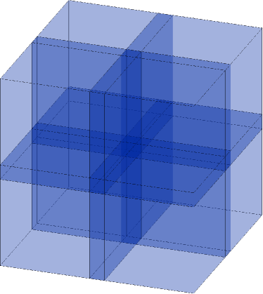
a) b)

Figure 4: The topological grid is subdivided into blocks, leaving an overlap of one cell in each direction (a). Cells inside regions of overlap (b) are assigned two different labels during the independent processing of the blocks. These labels are subsequently reconciled.

Step 1 (connected component labeling). The topological grid is subdivided into blocks such that each block begins and ends in each direction with a layer that contains 3-cells. Moreover, adjacent blocks are chosen to overlap each other by one cell in each direction as is depicted in Fig. 4. In consequence, each 1-cell and each 2-cell within a region of overlap belongs to two different blocks, cf. Fig. 4b. Each block is then labeled independently using the algorithms 1, 2, and 3, and the respective labelings are stored on the hard drive. In consequence, the labeling of connected components starts in each block with the label 1.

Step 2 (label disambiguation). The processed blocks are put in an arbitrary but fixed order. If the $j$-th block in this order contains $m_{2}$ 2-components, the offset $m_{2}$ is stored along with block $j+1$ where it is added on demand to all non-zero 2-cell labels, similarly for 1-cells and 0-cells, arriving at maximal labels $M_{0},M_{1},M_{2}$ of 0-, 1-, and 2-cells, respectively, for the entire volume.

Step 3 (label reconciliation). Whenever connected components of cells extend across block boundaries, their labels in the respective blocks (with offsets added) need to be reconciled. Two disjoint set data structures equipped with the operations union and find [18] are used for this purpose, one for 1-cells and one for 2-cells, the former with $M_{1}$, the latter with $M_{2}$ initially distinct sets, each set containing one label. First, union$(l_{1},l_{2})$ is called for the pair $(l_{1},l_{2})$ of distinct labels assigned to any active 1-cells and 2-cells within a region of overlap. Second, each label $l$ is replaced by the representative find$(l)$ of the union to which it belongs.

Step 4 (curve merging). As is elucidated in the correctness analysis of this algorithm in Section 5.1, 1-components can still be falsely split and 0-cells falsely labeled as active at this stage. Thus, in a last step, each 0-cell $t_{0}$ and any pair $(t_{1},t^{\prime}_{1})$ of 1-components bounded by $t_{0}$ is considered. The labels of $t_{1}$ and $t^{\prime}_{1}$ are reconciled if $t_{1}$ and $t^{\prime}_{1}$ bound the same connected components of 2-cells. If at least one reconciliation has taken place, the activity of $t_{0}$ is re-computed.

5.1 Correctness of the Algorithm

In order to prove that the block-wise processing is correct, the segment label map $\sigma$ as well as the decomposition of the topological grid into blocks are assumed to be arbitrary but fixed. The labeling $\tau^{\prime}$ output by the block-wise method is compared to the labeling $\tau$ obtained from the application of Algorithms 1, 2 and 3 to the entire segment label map. While the latter is known to be correct, the former is correct if the two labelings are isomorphic:

Definition 5

Two labelings $\tau,\tau^{\prime}:T\rightarrow\mathbb{N}$ of the topological grid $T$ are isomorphic w.r.t. a subset $U\subseteq T$ if and only if the following conditions hold:

$$\forall u\in U:\quad\tau(u)=0\Leftrightarrow\tau^{\prime}(u)=0\enspace,$$ (4)

$$\forall u,v\in U:\quad\tau(u)=\tau(v)\Leftrightarrow\tau^{\prime}(u)=\tau^{\prime}(v)\enspace.$$ (5)

If $\tau$ and $\tau^{\prime}$ are isomorphic w.r.t. the entire domain $T$, they are simply called isomorphic.

Proposition 1

$\tau$ and $\tau^{\prime}$ are isomorphic w.r.t. all 3-cells of $T$.

Proof

3-cell labels are copied from the segment label map $\sigma$ to $\tau$ and $\tau^{\prime}$, respectively by both algorithms. The labelings $\tau$ and $\tau^{\prime}$ are therefore identical and thus isomorphic w.r.t. all 3-cells of $T$.

Proposition 2

$\tau$ and $\tau^{\prime}$ are isomorphic w.r.t. all 2-cells of $T$.

Proof

During block-wise processing, the decision whether or not a 2-cell obtains a non-zero label depends exclusively on the labeling of 3-cells w.r.t. which $\tau$ and $\tau^{\prime}$ are identical. Thus, (4) holds for all 2-cells of $T$.

Let $u,v\in T$ be any 2-cells. If $\tau(u)\not=\tau(v)$, $u$ and $v$ bound different pairs of segments and hence obtain different labels during block-wise processing. Such labels are not reconciled. Thus, $\tau^{\prime}(u)\not=\tau^{\prime}(v)$.

If $\tau(u)=\tau(v)$, there exists a path of 2-cells between $u$ and $v$ on which all cells separate the same pair of segments. If this path is contained in one single block, all its 2-cells obtain the same label during the independent processing of that block. If the path crosses the boundaries of blocks, the labels along the path are reconciled. Thus, $\tau^{\prime}(u)=\tau^{\prime}(v)$.

Hence, (5) hold for all pairs of 2-cells. In conclusion, $\tau$ and $\tau^{\prime}$ are isomorphic w.r.t. all 2-cells of $T$.

Proposition 3

For each block $U\subseteq T$, any 1-cell $t_{1}\in U$, and any 2-cell $t_{2}\in\Gamma(t_{1})$, the label assigned to $t_{2}$ is unique among the labels assigned to all 2-cells in $\Gamma(t_{1})$ before label reconciliation if and only if it is unique afterwards.

Proof

($\Rightarrow$) Suppose $t_{2}$ had a unique label among the elements of $\Gamma(t_{1})$ before label reconciliation and the same label as another $t^{\prime}_{2}\in\Gamma(t_{1})$ afterwards, i.e. in $\tau^{\prime}$. Then, $t_{2}$ and $t^{\prime}_{2}$ separated the same pair of segments because $\tau^{\prime}$ is isomorphic to the correct labeling $\tau$ w.r.t the 2-cells. Moreover, we know by definition that $t_{2}\leftrightarrow t^{\prime}_{2}$, so $t_{2}$ and $t^{\prime}_{2}$ would have obtained the same label before label reconciliation. A contradiction. ($\Leftarrow$) Trivial.

Proposition 4

For all 1-cells $t_{1}\in T$ holds $\tau(t_{1})=0\Leftrightarrow\tau^{\prime}(t_{1})=0$.

Proof

During the independent processing of each block, any 1-cell $t_{1}\in T$ obtains a non-zero label if and only if at least one 2-cell label is unique among the labels assigned to all 2-cells of $\Gamma(t_{1})$. In this step, the 2-cell labels before label reconciliation are considered. However, by Prop. 3, this is no different than considering the 2-cell labels of $\tau^{\prime}$. Moreover, $\tau^{\prime}$ and $\tau$ are isomorphic w.r.t. all 2-cell and thus, 1-cells obtain a non-zero label in $\tau^{\prime}$ precisely if they are labeled non-zero in $\tau$, i.e. $\tau(t_{1})=0\Leftrightarrow\tau^{\prime}(t_{1})=0$.

Proposition 5

For all 1-cells $u,v\in T$ holds $\tau(u)=\tau(v)\Leftarrow\tau^{\prime}(u)=\tau^{\prime}(v)$.

Proof

If $\tau^{\prime}(u)=0$, the conjecture holds by virtue of Prop. 4. If $\tau^{\prime}(u)\not=0$, it follows that $\tau^{\prime}(v)\not=0$ (by assertion) as well as $\tau(u)\not=0$ and $\tau(v)\not=0$ (by Prop. 4). Moreover, $\tau^{\prime}(u)=\tau^{\prime}(v)$ requires by construction of $\tau^{\prime}$ that $u$ and $v$ are connected by a path of 1-cells all of which bound the same connected components of 2-cells (in $\tau^{\prime}$). As $\tau$ and $\tau^{\prime}$ are isomorphic w.r.t. the 2-cells and as 1-cells are labeled correctly in $\tau$, it follows that $\tau(u)=\tau(v)$.

Proposition 6

For all 0-cells $t\in T$ holds $\tau(t)\not=0\Rightarrow\tau^{\prime}(t)\not=0$.

Proof

If $\tau(t)\not=0$, at least one 1-cell label is non-zero and unique among the labels assigned to all 1-cells in $\Gamma(t)$, i.e.

$$\exists u\in\Gamma(t):\quad\tau(u)\not=0\wedge\forall v\in\Gamma(t)\setminus\{u\}:\tau(u)\not=\tau(v)\enspace.$$

For any such $u$ follows by Prop. 4 and 5

$$\tau^{\prime}(u)\not=0\wedge\forall v\in\Gamma(t)\setminus\{u\}:\tau^{\prime}(u)\not=\tau^{\prime}(v)$$

and thus, by construction of $\tau^{\prime}$, the conjecture.

In order to prove that $\tau$ and $\tau^{\prime}$ are isomorphic, it remains to be shown that the inverse implications of Prop. 5 and 6 also hold. Unlike the above propositions which hold by construction of $\tau^{\prime}$ in Steps 1–3 of the block algorithm, the two missing implications are enforced explicitly, by Step 4.

As the following example shows, 1-components can indeed be falsely split and 0-cells falsely labeled active if Step 4 is omitted. In Fig. 5a, a segment label map on a grid of $3\times 3\times 2$ voxels is shown. Six segments are identified by the integers $1$ through $6$. The correct corresponding topological label map is depicted in Fig. 5b, and the connected components are plotted in Fig. 6a and 6b. The 1-cell labels in Fig. 5b are colored in accordance with the graphical visualization in Fig. 6b.

Assume that the segment label map in Fig. 5a is processed block-wise, with blocks of $2\times 2\times 2$ voxels. Note that this block-size includes an overlap of one voxel in each direction. The bold font in Fig. 5a indicates one of these blocks. The topological label map that is constructed when this block is processed independently is depicted in Fig. 5c. While the 1-cells labeled 1 and 2 are merged into one connected component during label reconciliation after all blocks have been processed, the 1-cells labeled 3 and 4 are merged only in Step 4 of the algorithm. If Step 4 were omitted, the incorrect labeling shown in Fig. 6c would be computed.

a) z = 1 1 1 1 1 2 1 1 1 3 z = 2 4 4 4 4 5 4 4 4 6

b) z = 1 1 0 1 0 1 0 0 1 0 0 1 1 2 1 1 0 0 1 0 2 1 0 1 2 3 z = 2 3 0 3 0 3 0 0 1 0 0 3 1 4 1 3 0 0 1 0 2 3 0 3 2 5 z = 3 4 0 4 0 4 0 0 6 0 0 4 6 5 6 4 0 0 6 0 7 4 0 4 7 6

c) z = 1 2 1 1 1 0 2 1 2 3 z = 2 3 2 5 1 1 4 4 3 6 z = 3 5 7 4 7 0 8 4 8 6

Figure 5: a) A segment label map on a grid of $3\times 3\times 2$ voxels. b) The correct corresponding topological label map. Colors are in accordance with the 1-cells shown in Fig. 6b. c) The topological label map of the block depicted in bold font in (a). 1-cells are colored in accordance with Fig. 6c. The 1-cells labeled 1 and 2 are merged during label reconciliation while the 1-cells labeled 3 and 4 are merged in Step 4 of the block-wise processing.

a)                                      b)                                         c)

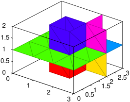
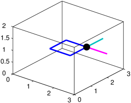
Figure 6: Connected components of 2-cells (a) and 1-cells (b) defined by the topological label map in Fig. 5b. c) 1-cells and the 0-cell from a block-wise labeling where Step 4 of the algorithm is omitted.

Theorem 5.1

$\tau$ and $\tau^{\prime}$ are isomorphic.

Proof

In addition to the implications proven above, Step 4 of the block-wise processing enforces:

(1) For all 1-cells $u,v\in T$ holds $\tau(u)=\tau(v)\Leftarrow\tau^{\prime}(u)=\tau^{\prime}(v)$.

(2) For all 0-cells $t\in T$ holds $\tau(t)\not=0\Leftarrow\tau^{\prime}(t)\not=0$.

By virtue of this theorem, the block-wise processing is correct.

5.2 Complexity

The runtime overhead introduced by the merging of labels is $O((N+M_{1}+M_{2})\log(M_{1}+M_{2}))$ where $N$ is the number of cells within regions of overlap. Time $O(N\log(M_{1}+M_{2}))$ is used for the $O(N)$ calls of union, whereas time $O((M_{1}+M_{2})\log(M_{1}+M_{2}))$ is required for the $M_{1}+M_{2}$ find-operations. In practice, this overhead is negligible compared to the runtime of the connected component labeling.

5.3 Parallelization

The algorithm can be used in two different settings: Blocks can be processed consecutively in order to extract the geometry of a large volume segmentation in limited RAM. Perhaps more interestingly, blocks can be processed in parallel, possibly on several machines, with virtually no process synchronization or inter-process communication.

Indeed, if it were not for parallelization, the block-wise connected component labeling could have been implemented simpler, starting with only the 2-cells, followed by the disambiguation and reconciliation of their labels across all blocks even before any 1-cell or 0-cell is labeled. This would render Step 4 of the block-wise processing unneccessary. However, the program would have to wait until the 2-cells of all blocks have been labeled before it could label the first 1-cell. In contrast, the proposed algorithm starts labeling the 1-cells within a block as soon as the labeling of 2-cells within that block is finished, regardless of the progress on other blocks.

6 Redundant Storage for Constant Time Access

The algorithm proposed in the last section labels segments, faces between segments, the curves between faces and the points between curves on the toplogical grid. The output is a topological label map that provides constant time access to the label at any topological coordinate. It allows to determine in constant time whether there is a face, curve, or point at a given location and if so, to determine its label. This is important, e.g. for the visualization of 2-dimensional slices of a segmentation that show not only segments but also faces, curves, and points. The algorithm makes explicit the bounding relations between the geometric objects.

However, not only the labels of individual cells and the adjacency of geometric objects are important but also the set of all cells that belong to the same component. For image analysis, it can for instance be useful to compute the mean gray value over a face between two segments. Yet, a list of all 2-cells of the face cannot be obtained in constant time from the topological grid labeling. Thus, a redundant representation of geometry is constructed that contains for each $j$-component a list of all its $j$-cells.

This redundant representation as well as the topological grid labeling are stored on the hard drive using the Hierarchical Data Format (HDF5). HDF5 was originally developed by the National Center for Supercomputing Applications (NCSA) and is now maintained by the non-profit HDF5-Group. It is widely used, especially in the life sciences [19]. An HDF5 file contains two principal types of objects, groups and datasets. Datasets represent the actual storage containers and are multi-dimensional arrays of a unique type, while groups represent an organizational concept analogous to a directory that enables the user to hierarchically structure the data within the file. Furthermore, attributes may be assigned to any dataset or group and contain meta information pertaining to the data stored within these objects.

Two HDF5 files are used here. The first file is associated with the labeling algorithm of Section 5. Its structure is depicted in Fig. 7a. For each block and its index $j$ in the order of blocks, a sub-group named $j$ is created in the group blocks. The sub-group $j$ contains the dataset topological-grid, a 3-dimensional array that stores the topological label map of the block. Furthermore, it contains datasets for the neighborhood relations of connected components as well as the label offsets of the block which are computed during label disambiguation. During label reconciliation, the datasets relabeling-$k$ and neighborhood-$k$ are created in the main file to store the labeling and the neighborhood relations of $k$-components of the entire topological grid.

a)                              b)

$t$	$d$	Name
D	1	segmentation-shape
D	1	block-shape
G		blocks
G		$\langle b\rangle$
D	3	topological-grid
D	1	max-labels
D	1	label-offsets
D	2	neighborhood-0
D	2	neighborhood-1
D	2	neighborhood-2
D	1	max-labels
D	1	relabeling-1
D	1	relabeling-2
D	2	neighborhood-0
D	2	neighborhood-1
D	2	neighborhood-2

$t$	$d$	Name
A	1	number-of-bins
D	1	segmentation-shape
D	1	max-labels
D	2	0-cells
G		1-components
G		bin-$\langle b\rangle$
D	2	$\langle q\rangle$-$\langle p\rangle$
G		2-components
G		bin-$\langle b\rangle$
D	2	$\langle q\rangle$-$\langle p\rangle$
G		3-components
G		bin-$\langle b\rangle$
D	2	$\langle q\rangle$-$\langle p\rangle$
D	1	parts-counters-1
D	1	parts-counters-2
D	1	parts-counters-3

Figure 7: Two HDF5 files store the information extracted during block-wise processing. Along with each data item, its type $t$ (a group $G$, a dataset $D$, or an attribute $A$) and dimension $d$ are shown. a) The 1st file provides constant-time access to the label of any cell as well as to the neighborhoods of connected components of cells. b) The 2nd file provides constant-time access to the coordinate lists of entire segments, faces and curves.

Using this file, constant time access to the label of a given cell works as follows. After identifying a block $k$ to which the $j$-cell of interest belongs, the label $l$ is read off from the dataset topological-grid of that block. Except for 3-cells and inactive cells, the offset $m$ associated with cell order $j$ and block $k$ is loaded and the dataset relabeling-$j$ accessed at location $l+m$ for the globally consistent label of the cell. In practice, all data except the topological label map can be kept in RAM.

The second HDF5 file stores one coordinate list for each 1-, 2-, and 3-component as well as the coordinates of all active 0-cells. Initially, the most straight forward group hierarchy was chosen for this file: Three groups associated with segments, faces, and curves, each containing one extendible dataset for each component. In addition, the coordinates of all 0-cells were stored in one 2-dimensional array. This group hierarchy turned out to be problematic when more than 10⁶ datasets were created per group, using version 1.8.4 of the HDF5 library. To overcome this problem, the more complex group hierarchy shown in Fig. 7b is used instead. In each of the groups 1-components, 2-components, and 3-components, a fixed number of sub-groups is created into which datasets containing coordinates lists are distributed. Also for performance reasons, the use of extendible datasets was dropped, which means that due to the block-wise nature of the algorithm, one complete $j$-component may be associated with several datasets representing its fragments from different blocks. The HDF5 file contains the datasets parts-counters-$j$ for the number of datasets a single $j$-connected is split into.

6.1 Alternatives

A more obvious way to store the coordinate lists is to create one binary file for each list. The use of many files offers the advantage that the coordinate lists may easily be extended by appending to files, an important asset for block-wise processing. However, bearing in mind that a segmentation of 2,000³ voxels easily contains in excess of $10^{6}$ connected components, the vast amount of files places a heavy burden on the file system, making simple operations such as copying the data extremely time consuming. In contrast, HDF5 was designed to organize large numbers of binary datasets.

A good alternative to HDF5 is a relational database. Experiments with a PostgreSQL database showed promising performance. This approach was nevertheless abandoned in favor of HDF5 because the necessity to install and configure a database might deter potential users from trying out the software.

7 Conclusion

In this article, a new algorithm for geometry and topology extraction from large volume segmentations is proposed. In contrast to previous methods, this algorithms processes volume segmentations in a block-wise fashion. This facilitates geometry and topology extraction from large volume segmentations with limited RAM and in parallel. The geometry is stored in HDF5 files that provide constant time access to the labels of segments, faces between segments, curves between faces and points between curves at any location as well as to lists of coordinates that constitute these objects. This representation makes a geometric analysis of large volume segmentations practical.

Appendix 0.A Compiling and Installing the Software

The CGP software is provided as C++ source code with a CMake 2.6 build system for the command line tools cgpx and cgpr as well as for MATLAB mex files. CGP depends on the HDF5 Library (version 1.8.4 or higher and can optionally make use of the Message Passing Interface (MPI), and the Visualization Toolkit vtk, . An example segmentation of $50\times 50\times 50$ voxels is included, along with the according outputs of cgpx and cgpr. The following paragraphs describe how CGP can be compiled on a system that has HDF5 installed.

0.A.1 Linux/UNIX and GNU C++

Unpack the source archive and create a build directory. Execute CMake in this directory, providing the path to the source as the last parameter:

unzip cgp.zip
mkdir build-cgp && cd build-cgp
CMake ../cgp
make

If HDF5, MATLAB, or vtk are installed in a non-standard way, CMake will not find them automatically. In this case, paths to include files and libraries need to be set manually in the above call, e.g. for HDF5:

CMake -DHDF5_INCLUDE_DIR=$HOME/inc \
  -DHDF5_LIBRARY=$HOME/lib/libhdf5.so \
  ../cgp

0.A.2 Microsoft Windows and VisualStudio

Unpack the source archive, create a build directory, and use the CMake GUI to configure. If CMake does not find HDF5, MATLAB, or vtk although they are installed, set the include paths and library paths for these packages manually. CMake will generate a VisualStudio solution file. Open this file, build the target ALL_BUILD in release mode, and install the binaries by building the target INSTALL.

Appendix 0.B Using the Software

0.B.1 From the Command Line

The command line tools cgpx and cgpr compute a representation of the geometry and topology of a volume segmentation. The segmentation needs to be stored as a 3-dimensional array of 32-bit unsigned integers in one dataset in the root group of an HDF5 file. The command line tools are then used as follows:

cgpx $\langle input\ file\rangle$ $\langle dataset\rangle$ $\langle b1\rangle$ $\langle b2\rangle$ $\langle b3\rangle$ $\langle output\ file\rangle$

cgpr $\langle input\ file\rangle\ \langle output\ file\rangle$.

The first tool constructs a labeled topological grid in a block-wise fashion using the block shape $b1\times b2\times b3$. The second tool writes a list of topological coordinates for each geometric object. Suppose, as an example, that a segmentation of 2,000³ voxels is stored as a 3-dimensional array in the dataset seg of the HDF5 file segmentation.h5. On a desktop computer equipped with 2 GB of RAM, a block-size of $200^{3}$ voxels is reasonable, so a representation of the geometry and topology of the segmentation can be obtained like this:

cgpx segmentation.h5 seg 200 200 200 grid.h5
cgpr grid.h5 objects.h5

In order to process several blocks in parallel, invoke the command line tool cgpx via mpiexec, e.g.

mpiexec -n 2 cgpx segmentation.h5 seg
  200 200 200 grid.h5

0.B.2 From MATLAB

In MATLAB, segmentations are conveniently stored as 3-dimensional arrays whose entries are 32-bit unsigned integers that correspond to segment labels. In order to extract the geometry and topology from a segmentation, the array has to be written to an HDF5 file by means of the function cgp_save. The following call of cgp_save writes the array $S$ as the dataset seg into the HDF5 file seg.h5:

cgp_save(’seg.h5’, ’/seg’, S);
Geometry and topology extraction can now be performed either from the command line, using the tools cgpx and cgpr as described in Section 0.B.1, or directly from MATLAB, using the according mex-functions:

cgpx(’seg.h5’, ’seg’, uint32([b1 b2 b3]),
  ’grid.h5’);
cgpr(’grid.h5’, ’objects.h5’);

where $b1\times b2\times b3$ specifies the block shape.

A number of functions named with the prefix cgp can be used to selectively load data from the geometry file. In the following example, one curve and its adjacent faces are plotted.

desc = cgp_open(’objects.h5’);
curve_id = 100;
hold on;
tcl = cgp_load_object(desc, 1, curve_id);
cgp_plot_1cells(tcl);
neighbors = desc.neighborhoods{2}(curve_id,:);
for j = 1:length(neighbors)
  if neighbors(j) == 0
      break;
  end
  tcl = cgp_load_object(desc,2,neighbors(j));
  tri = cgp_triangulate(tcl);
  cgp_plot_triangulation(tri, rand(1,3),0.7);
end
hold off;
cgp_close(desc);

A 0-cell and its adjacent curves are plotted as follows:

desc = cgp_open(’objects.h5’);
point_id = 100;
hold on;
tcl = cgp_load_object(desc, 0, point_id);
cgp_plot_0cells(tcl);
neighbors = desc.neighborhoods{1}(point_id,:);
for j = 1:length(neighbors)
  if neighbors(j) == 0
      break;
  end
  tcl = cgp_load_object(desc,1,neighbors(j));
  cgp_plot_1cells(tcl, rand(1,3));
end
hold off;
cgp_close(desc);

0.B.3 From C++

The C++ API for parallelized geometry and topology extraction is defined in the header files cgp_hdf5.hxx, CgpxMaster.hxx, and CgpxWorker.hxx. The construction of the topological grid is invoked by classes

template<class T, class C> class CgpxMaster;
template<class T, class C> class CgpxWorker;

that implement a master-worker-scheme using MPI. The type $T$ is used for labels of geometric objects; unsigned integers of at least 32 bits should be used. The type $C$ is used for coordinates to navigate in arrays. 16-bit integers are sufficient if the segmentation is smaller than 32769 voxels in each dimension.

The coordinate lists of all geometric objects can be constructed from the topological grid by means of the function

template<class T, class C>
void geometry3blockwise(
  const hid_t&, // input HDF5 file
  const hid_t&  // output HDF5 file
);

The source files of the command line tools,

src/cmd/cgpx.cxx
src/cmd/cgpr.cxx

show the interested reader how the classes and function are used.

References

- [1] Brice, C.R., Fennema, C.L.: Scene analysis using regions. Artificial Intelligence 1 (1970) 205–226
- [2] Pavlidis, T.: Structural Pattern Recognition. Volume 1 of Electrophysics. Springer (1977)
- [3] Kovalevsky, V.A.: Finite topology as applied to image analysis. Computer Vision, Graphics, and Image Processing 46 (1989) 141–161
- [4] Kovalevsky, V.A.: Digital geometry based on the topology of abstract cell complexes. In: Proceedings of the DGCI 1993. (1993) 259–284
- [5] Khalimsky, E., Kopperman, R., Meyer, P.: Computer graphics and connected topologies on finite ordered sets. Topology and its Applications 36 (1990) 1–17
- [6] Meine, H., K the, U.: The GeoMap: A unified representation for topology and geometry. In Brun, L., Vento, M., eds.: Graph-Based Representations in Pattern Recognition. LNCS 3434, Springer (2005) 132–141
- [7] Damiand, G.: Topological model for 3D image representation: Definition and incremental extraction algorithm. Computer Vision and Image Understanding 109 (2008) 260–289
- [8] Kropatsch, W.G.: Building irregulars pyramids by dual graph contraction. Proceedings of the IEEE Conference on Vision, Image and Signal Processing 142 (1995) 366–374
- [9] Braquelaire, J.P., Guitton, P.: 2 1/2d scene update by insertion of contour. Computers and Graphics 15 (1991) 41–48
- [10] Lienhardt, P.: Subdivisions of n-dimensional spaces and n-dimensional generalized maps. In: Proceedings of the 5th annual symposium on computational geometry, New York, NY, USA, ACM (1989) 228–236
- [11] Lienhardt, P.: Topological models for boundary representation: a comparison with n-dimensional generalized maps. Computer Aided Design 23 (1991) 59–82
- [12] Bertrand, Y., Damiand, G., Fiorio, C.: Topological encoding of 3D segmented images. In Borgefors, G., Nystr m, I., Sanniti di Baja, G., eds.: Proceedings of the DGCI 2000. LNCS 1953, Springer (2000) 311–324
- [13] Damiand, G., Resch, P.: Split and merge algorithms defined on topological maps for 3D image segmentation. Graphical Models 65 (2003) 149–167
- [14] Munkres, J.R.: Elements of Algebraic Topology. Perseus Books (1995)
- [15] Hatcher, A.: Algebraic topology. Cambridge University Press (2002)
- [16] Klette, R.: Cell complexes through time. In Latecki, L.J., Mount, D.M., Wu, A.Y., eds.: Vision Geometry IX. Volume 4117., Society of Photo-Optical Instrumentation Engineers (SPIE) (2000) 134–145
- [17] Meine, H., K the, U., Stiehl, H.: Fast and accurate interactive image segmentation in the geomap framework. In Tolxdorff, T., Braun, J., Handels, H., Horsch, A., Meinzer, H.P., eds.: Proc. Bildverarbeitung f r die Medizin, Springer (2004) 60–64
- [18] Cormen, T.H., Leiserson, C.E., Rivest, R.L., Stein, C.: 21. Data structures for disjoint sets. In: Introduction to Algorithms. 3rd edn. MIT Press (2009) 498–524
- [19] Dougherty, M.T., Folk, M.J., Zadok, E., Bernstein, H.J., Bernstein, F.C., Eliceiri, K.W., Benger, W., Best, C.: Unifying biological image formats with hdf5. Commun. ACM 52 (2009) 42–47