Discrete primitive-stable representations with large rank surplus

Abstract.

We construct a sequence of primitive-stable representations of free groups into $PSL_{2}(\mathbb{C})$ whose ranks go to infinity, but whose images are discrete with quotient manifolds that converge geometrically to a knot complement. In particular this implies that the rank and geometry of the image of a primitive-stable representation imposes no constraint on the rank of the domain.

1. Introduction

Let $F_{n}$ denote the free group on $n$ generators, where $n\geq 2$. The space $Hom(F_{n},PSL_{2}(\mathbb{C}))$ of representations of $F_{n}$ into $PSL(2,\mathbb{C})$ contains within it presentations of all hyperbolic 3-manifold groups of rank bounded by $n$, and so is of central interest in three-dimensional geometry and topology. On the other hand there is also an interesting dynamical structure on $Hom(F_{n},PSL_{2}(\mathbb{C}))$ coming from the action of $Aut(F_{n})$ by precomposition (see Lubotzky [11]). The interaction between the geometric and dynamical aspects of this picture is still somewhat mysterious, and forms the motivation for this paper.

(Note that it is natural to identify representations conjugate in $PSL_{2}(\mathbb{C})$, so that in fact we often think about the character variety ${\mathcal{X}}(F_{n})$ and the natural action by $Out(F_{n})$, the outer automorphism group of $F_{n}$. This distinction will not be of great importance here.)

In [15] the notion of a primitive-stable representation $\rho:F_{n}\to PSL_{2}(\mathbb{C})$ was introduced. The set $PS(F_{n})\subset{\mathcal{X}}(F_{n})$ of primitive stable conjugacy classes is open and contains all Schottky representations (discrete, faithful representations with compact convex core), but it also contains representations with dense image, and nevertheless $Out(F_{n})$ acts properly discontinuously on $PS(F_{n})$. This implies, for example, that $Out(F_{n})$ does not act ergodically on the (conjugacy classes of) representations with dense image.

Representations into $PSL_{2}(\mathbb{C})$, whose images are discrete, torsion-free subgroups, give rise to hyperbolic 3-manifolds, and when the volume of the 3-manifold is finite we know by Mostow-Prasad rigidity that the representation depends uniquely, up to conjugacy, on the presentation of the abstract fundamental group. Hence it makes sense to ask whether a presentation of such a 3-manifold group is or is not primitive-stable.

It is not hard to show that primitive-stable presentations of closed 3-manifold groups do exist, and such presentations are constructed in this paper, but we are moreover concerned with the relationship between the rank of the presentation and the rank of the group.

Our goal will be to show that the rank of the presentation can in fact be arbitrarily higher than the rank of the group, and more specifically:

Theorem 1.1.

There is an infinite sequence of representations $\rho^{r}:F_{n_{r}}\to PSL_{2}(\mathbb{C})$, where $n_{r}=n_{0}+2r$, so that :

1. Each $\rho^{r}$ has discrete and torsion-free image.

2. Each $\rho^{r}$ is primitive-stable.

3. The quotient manifolds $N_{r}=\mathbb{H}^{3}/\rho^{r}(F_{n_{r}})$ converge geometrically to $N_{\infty}$, where $N_{\infty}$ is a knot complement in $S^{3}$.

In particular note that, because the quotient manifolds converge geometrically to a fixed finite volume limit, the rank as well as the covolume of the image groups remains bounded while $n_{r}\to\infty$ (see e.g. Thurston [19]), hence:

Corollary 1.2.

There exists $R$ such that, for each $n$, there is a lattice in $PSL_{2}(\mathbb{C})$ with rank bounded by $R$, which is the image of a primitive stable representation of rank greater than $n$.

As the reader might guess our construction involves a sequence of Dehn fillings of a knot complement, and in particular the manifolds $N_{r}$ are in infinitely many homemorphism types. Thus we are currently unable to answer the following natural question:

Question 1.3.

Is there a single lattice $G\subset PSL_{2}(\mathbb{C})$ which has primitive stable presentations of arbitrarily high rank?

To put this in context we note that (as follows from the results in [15]) simply adding generators to a representation which map to the group generated by the previous generators immediately spoils the property of primitive stability. Thus the existence of primitive stable presentations is delicate to arrange.

On the other hand, we do not have examples in the other direction either:

Question 1.4.

Are there any lattices in $PSL_{2}(\mathbb{C})$ which do not have any primitive stable presentations?

The only tool we have for proving primitive-stability involves Heegaard splittings which must satisfy a number of interacting conditions. It would be interesting to know if this is always the case:

Question 1.5.

Is every primitive stable presentation of a closed hyperbolic 3-manifold group geometric, i.e. does it arise from one side of a Heegaard splitting?

Outline of the construction

Our starting point is a class of knots supported on surfaces in $S^{3}$ in a configuration known as a trellis, as previously studied by Lustig-Moriah [12]. The surface $\Sigma$ on which such a knot $K$ is supported splits $S^{3}$ into two handlebodies. For appropriately chosen special cases we find that the complement $S^{3}\smallsetminus K$ is hyperbolic, and that the representation obtained from one of the handlebodies is primitive stable. Most of the work for this is done in Section 5, about which we remark more below.

To our chosen examples we can apply flype moves (as used by Casson-Gordon, see Moriah-Schultens [17, Appendix]), which are isotopies of the knot that produce new trellis projections, with higher genus. We show that these new projections still yield primitive stable representations.

Hence our knot complement $S^{3}\smallsetminus K$ admits a sequence of homomorphisms $\rho^{r}_{\infty}:F_{n_{r}}\to\pi_{1}(S^{3}\smallsetminus K)$ with ranks $n_{r}\to\infty$, all of which are primitive stable. However, these maps are not surjective.

To address this issue we perform Dehn fillings on $S^{3}\smallsetminus K$, obtaining closed manifolds equipped with surjective homomorphisms from $F_{n_{r}}$. Thurston’s Dehn Filling Theorem tells us that, fixing the flype index $r$ and letting the Dehn filling coefficient go to infinity, we eventually obtain hyperbolic manifolds, and the corresponding representations $\rho^{r}_{m}$ converge to $\rho^{r}_{\infty}$. Since primitive stability is an open condition we eventually obtain our desired primitive stable presentations.

Section 2 provides a little bit of background on hyperbolic 3-manifolds. In Section 3, we discuss primitive stability and prove Proposition 3.5, which gives topological conditions for primitive stability of a representation arising from a Heegaard splitting where a knot on the Heegaard surface has been deleted. The proof of this is an application of Thurston’s covering theorem, and of the main result of [15].

In Section 4 we introduce trellises and our notation for knots carried on them, recall a theorem from Lustig-Moriah [12], and discuss horizontal surgeries.

In Section 5 we show that, under appropriate assumptions, a knot carried by a trellis satisfies the conditions of Proposition 3.5, and moreover the same is true for the configurations obtained by flype moves on this knot. Theorem 5.2 establishes that the knot complements we work with are hyperbolic. Intuitively one expects that complicated diagrams such as we are using should “generically” yield hyperbolic knots, but the proof turns out to be somewhat long and painful. We perform a case-by-case analysis of the features of the knot diagram, which is complicated by various edge effects in the trellis. This analysis shows that the manifold has no essential tori, and the same techniques also apply, in Proposition 5.10, to show that the exterior pared handlebody determined by a flyped trellis is never an $I$-bundle, which is also one of the conditions needed in Proposition 3.5.

The level of generality we chose for our family of examples, for better or worse, is restricted enough to simplify some of the arguments in Section 5, but still broad enough to allow a wide variation. It is fairly clear that the construction should work for an even wider class of examples, but satisfying primitive stability, hyperbolicity, as well as the no-$I$-bundle condition is tricky and the resulting complication of our arguments would have diminishing returns for us and our readers.

2. Cores and ends of hyperbolic manifolds

In this section we review the basic structure of hyperbolic 3-manifolds and their ends. This will be applied in Section 3.

A compact core of a 3-manifold $N$ is a compact submanifold $C$ of $N$ whose inclusion is a homotopy-equivalence. Scott [18] showed that every irreducible 3-manifold with finitely generated fundamental group has a compact core.

Let $N=\mathbb{H}^{3}/\Gamma$ be an oriented hyperbolic 3-manifold where $\Gamma$ is a discrete torsion-free subgroup of $PSL_{2}(\mathbb{C})$, and let $N^{0}$ denote $N$ minus its standard (open) cusp neighborhoods. Each cusp neighborhood is associated to a conjugacy class of maximal parabolic subgroups of $\Gamma$, and its boundary is an open annulus or a torus. For each component $T$ of $\partial N^{0}$ let $T^{\prime}$ be an essential compact subannulus when $T$ is an annulus, and let $T^{\prime}=T$ if $T$ is a torus.

The relative compact core theorem of McCullough [13] and Kulkarni-Shalen [10] implies:

Theorem 2.1.

There is a compact core $C\subset N^{0}$, such that $\partial C\cap T=T^{\prime}$ for every component of $\partial N^{0}$.

We call $C$ a relative compact core, and call $P=\partial C\cap\partial N^{0}$ the parabolic locus on its boundary. The pair $(C,P)$ is called a pared manifold (see Morgan [16]).

Suppose that the components of $\partial C\smallsetminus P$ are incompressible. Then Bonahon showed in [2] that the components of $N^{0}\smallsetminus C$ are in one-to-one correspondence with the components of $\partial C\smallsetminus P$, and each of them is a neighborhood of a unique end of $N^{0}$. Note that $C$ can be varied by isotopy and by choice of the annuli $T^{\prime}$, so that an end can have many neighborhoods.

We say that an end of $N^{0}$ is geometrically finite if it has a neighborhood which is entirely outside of the convex core of $N$ (where the convex core of $N$ is the smallest closed convex subset of $N$ whose inclusion is a homotopy equivalence).

Bonahon’s tameness theorem [2] shows that every end of $N^{0}$ is either geometrically finite or simply degenerate. We will not need the definition of this property, but will use the fact that it has Thurston’s Covering Theorem as a consequence. The Covering Theorem will be described and used in the proof of Proposition 3.5.

We remark that something similar to all this holds when $\partial C\smallsetminus P$ is compressible via the solution to the Tameness Conjecture by Agol [1] and Calegari-Gabai [4], but we will not need to use this.

3. Primitive stable representations

In this section we summarize notation and facts from [15], and prove Proposition 3.5, which gives a sufficient condition for certain representations arising from knot complements to be primitive stable.

Fix a generating set $\{X_{1},\ldots,X_{n}\}$ of $F_{n}$ and let $\Gamma$ be a bouquet of oriented circles labeled by the $X_{i}$. We let $\mathcal{B}=\mathcal{B}(\Gamma)$ denote the set of bi-infinite (oriented) geodesics in $\Gamma$. Each such geodesic lifts to an $F_{n}$-invariant set of bi-infinite geodesics in the universal covering tree $\tilde{\Gamma}$. The set $\mathcal{B}$ admits a natural action by $Out(F_{n})$.

An element of $F_{n}$ is called primitive if it is a member of a free generating set, or equivalently if it is the image of a generator $X_{i}$ by an element of $Aut(F_{n})$. Let $\mathcal{P}=\mathcal{P}(F_{n})$ denote the subset of $\mathcal{B}$ consisting of geodesic representatives of conjugacy classes of primitive elements. Note that $\mathcal{P}$ is $Out(F_{n})$-invariant.

Given a representation $\rho:F_{n}\to PSL_{2}(C)$ and a basepoint $x\in\mathbb{H}^{3}$, there is a unique map $\tau_{\rho,x}:\tilde{\Gamma}\to\mathbb{H}^{3}$ mapping a selected vertex of $\tilde{\Gamma}$ to $x$, $\rho$-equivariant, and mapping each edge to a geodesic.

Definition 3.1.

A representation $\rho:F_{n}\to PSL_{2}(C)$ is primitive-stable if there are constants $K,\delta\in\mathbb{R}$ and a basepoint $x\in\mathbb{H}^{3}$ such that $\tau_{\rho,x}$ takes the leaves of $\mathcal{P}$ to $(K,\delta)$-quasi geodesics in $\mathbb{H}^{3}$.

The property of primitive stability of a representation is invariant under conjugacy in $PSL_{2}(C)$ and action by $Aut(F_{n})$. We define $\mathcal{PS}(F_{n})$ to be the set of (conjugacy classes of) primitive-stable representations.

It is easy to see that Schottky representations are primitive stable; indeed, the Schottky condition is equivalent to saying that the map $\tau_{\rho,x}$ is a quasi-isometric embedding on the entire tree at once.

Definition 3.2.

Given a free group $F(X)=F(X_{1},\dots,X_{n})$ on $n$ generators and a cyclically reduced word $w=w(X_{1},\dots,X_{n})$ the Whitehead graph of $w$ with respect to the generating set $X$, denoted $Wh(w,X)$, is defined as follows: The vertex set of the graph consists of $2n$ points labeled by the elements of $X^{\pm}\equiv\{X_{i}^{\pm 1}\}$. For each sub-word $UV$ in $w$ or its cyclic permutations, where $U,V\in X^{\pm}$, we place an edge between the points $U$ and $V^{-1}$.

Definition 3.3.

We say that a graph $\Gamma$ is cut point free if it is connected and contains no point $p\in\Gamma$ so that $\Gamma\smallsetminus p$ is not connected.

It is a theorem of Whitehead [21, 22] that if $u\in F_{n}$ is a cyclically reduced primitive word then $Wh(u,X)$ is not cut point free.

If $H$ is a handlebody and $\gamma$ is a curve in $\partial H$, for a generating system $X$ for $\pi_{1}(H)$ let $Wh(\gamma,X)$ denote $Wh([\gamma],X)$, where $[\gamma]$ is a reduced word in $X^{\pm}$ representing $\gamma$ in $\pi_{1}(H)$.

The main result of [15] states:

Theorem 3.4.

[Theorem 4.1 of [15]] If $\rho:\pi_{1}(H)\to PSL_{2}(\mathbb{C})$ is discrete, faithful and geometrically finite, with a single cusp $c$ such that $Wh(c,X)$ is cut-point free for some set of generators $X$ of $\pi_{1}(H)$, then $\rho$ is primitive stable.

This theorem will allow us to prove the following proposition, which in turn will be a step in the proof of Theorem 1.1. Here and in the rest of the paper, we let $\overline{\mathcal{N}}_{X}(Y)$ denote a closed regular neighborhood of $Y$ in $X$, and $\mathcal{N}_{X}(Y)$ its interior. If the ambient space $X$ is understood we abbreviate to $\mathcal{N}(Y)$. When we say a manifold with boundary is hyperbolic we mean its interior admits a complete hyperbolic structure.

Proposition 3.5.

Let $M$ be a closed $3$-manifold with a Heegaard splitting $M=H_{1}\cup_{\Sigma}H_{2}$, where $\Sigma=\partial H_{1}=\partial H_{2}$. Let $\gamma\subset\Sigma$ be a simple closed curve so that $M_{\infty}=M\smallsetminus\operatorname{\mathcal{N}}(\gamma)$ is a hyperbolic manifold and:

1. The group $\pi_{1}(H_{1})$ has a generating set $x=\{x_{1},\dots.x_{n}\}$ so that the Whitehead graph $Wh(\gamma,x)$ is cut point free.

2. The subsurface $\overline{\Sigma\smallsetminus\operatorname{\mathcal{N}}(\gamma)}$ is incompressible in $M_{\infty}$.

3. The pared manifold $(H_{2},\overline{\mathcal{N}}_{\Sigma}(\gamma))$ is not an $I$-bundle.

Let $\widehat{H_{1}}=H_{1}-\operatorname{\mathcal{N}}(\gamma)$ and let $\,\,i^{0}:\widehat{H_{1}}\to M_{\infty}$ be the map induced by the inclusion of $H_{1}\to M$ and $\eta:\pi_{1}(M_{\infty})\to PSL_{2}(\mathbb{C})$ be a holonomy representation for the hyperbolic structure on $int(M_{\infty})$. Then the representation $\rho=\eta\,\circ\,i^{0}_{*}$ given by

$$\pi_{1}(\widehat{H}_{1})\overset{i^{0}_{*}}{\to}\pi_{1}(M_{\infty})\overset{\eta}{\to}PSL_{2}(\mathbb{C})$$

is primitive stable.

Since $\widehat{H}_{1}$ is a deformation retract of $H_{1}$ we can naturally identify $\pi_{1}(H_{1})$ with $\pi_{1}(\widehat{H}_{1})$.

Recall that in a pared manifold $(M,P)$ (where $P\subset\partial M$ is a union of annuli and tori), an essential annulus is a properly embedded $\pi_{1}$ injective annulus in $(M,\partial M\smallsetminus P)$ which is not properly homotopic into $P$ or into $\partial M\smallsetminus P$. We say that $(M,P)$ is acylindrical if it contains no essential annuli.

We will need the following lemma:

Lemma 3.6.

Let $M$ be a closed $3$-manifold with a Heegaard splitting $M=H_{1}\cup_{\Sigma}H_{2}$, where $\Sigma=\partial H_{1}=\partial H_{2}$. Let $\gamma\subset\Sigma$ be a simple closed curve such that the subsurface $\Sigma\smallsetminus\operatorname{\mathcal{N}}(\gamma)$ is incompressible in $M_{\infty}$. Suppose that $M_{\infty}=M\smallsetminus\operatorname{\mathcal{N}}(\gamma)$ is a hyperbolic manifold and $\rho:\pi_{1}(M_{\infty})\to PSL_{2}(\mathbb{C})$ is a corresponding holonomy representation. Then the group generated by the element $\rho([\gamma])$ is up to conjugacy the unique maximal parabolic subgroup in $\rho(\pi_{1}(H_{1}))$.

Perhaps surprisingly, we are not assuming that $\Sigma\smallsetminus\mathcal{N}(\gamma)$ is acylindrical in either $H_{1}$ or $H_{2}$. Instead, the compressibility of the handlebodies plays an important role.

Proof.

The relative core theorem (Theorem 2.1), applied to the manifold $N=\mathbb{H}^{3}/\rho(\pi_{1}(H_{1}))$, gives a compact core $C_{1}\subset N$ such that the parabolic conjugacy classes of $\rho(\pi_{1}(H_{1}))$ are represented by a system of disjoint closed curves on $\partial C_{1}$. The lift to $N$ of $H_{1}$ is also a compact core, hence it is homeomorphic to $C_{1}$, by a map which induces $\rho$ on $\pi_{1}(H_{1})$ (Theorems 1 and 2 of McCullough-Miller-Swarup [14]). It follows that the generators of parabolic subgroups of $\rho|_{\pi_{1}(H_{1})}$ are also represented by a disjoint collection of simple closed loops $\beta_{1},\ldots,\beta_{k}$ on $\Sigma=\partial H_{1}$, where $\gamma=\beta_{1}$.

Choose some $\beta=\beta_{i}$. Since the only parabolic conjugacy classes in $\pi_{1}(M_{\infty})$ are the elements in $\pi_{1}(\partial M_{\infty})$, there is a singular annulus $\alpha:S^{1}\times[0,1]\to M_{\infty}$ which on $a_{0}\equiv S^{1}\times\{0\}$ is a parametrization of $\beta$, and maps $a_{1}\equiv S^{1}\times\{1\}$ to $\partial M_{\infty}$.

Perturb $\alpha$, if need be, so that $\alpha\pitchfork\Sigma\smallsetminus\mathcal{N}(\gamma)$, and choose it to minimize the number of components of $\alpha^{-1}(\Sigma)$. Now using the fact that $\Sigma\smallsetminus\mathcal{N}(\gamma)$ is incompressible in $M_{\infty}$, we may assume that all components of $\alpha^{-1}(\Sigma)$ are essential simple closed curves in $S^{1}\times[0,1]$, or arcs in $S^{1}\times[0,1]$ with both end points on $a_{1}$. We will next show that such arcs do not occur.

Let $\delta\subset S^{1}\times[0,1]$ be an outermost arc of $\alpha^{-1}(\Sigma)$. The points $\partial\delta$ bound an arc $\delta^{\prime}\subset a_{1}$ such that $\delta\cup\delta^{\prime}$ bounds a disk $\Delta\subset S^{1}\times[0,1]$. The image $\alpha(\Delta)$ is contained in exactly one of either $H_{1}$ or $H_{2}$, call it $H_{k}$.

Let $B$ be the annulus $\partial M_{\infty}\cap H_{k}$. The arc $\delta^{\prime}$ is properly embedded in $B$. If its endpoints are on the same component of $\partial B$, we could homotope $\delta^{\prime}$ rel endpoints to $\partial B$. This allows us deform $\alpha$ in a neighborhood of $\delta^{\prime}$, so that $\alpha^{-1}(\Sigma)$ in a neighborhood of $\Delta$ becomes a closed loop. This loop can be removed, again because $\Sigma\smallsetminus\mathcal{N}(\gamma)$ is incompressible, contradicting the choice of $\alpha$.

If the endpoints of $\delta^{\prime}$ are on different components of $\partial B$, let $\gamma^{\prime}$ be a core of $B$. Then the singular disk $\alpha(\Delta)$, after a homotopy near $\delta^{\prime}$, intersects $\gamma^{\prime}$ in a single point. In other words, $\gamma^{\prime}$ is primitive in $\widehat{H}_{k}=H_{k}\smallsetminus\mathcal{N}(\gamma)$, i.e. it is isotopic to the core of a 1-handle. That would imply that the surface $\Sigma\smallsetminus\mathcal{N}(\gamma)$ is compressible in $H_{k}$, in contradiction to assumption $(2)$. We conclude that $\alpha^{-1}(\Sigma)$ contains no arc components.

The essential simple closed curves in $\alpha^{-1}(\Sigma)$ partition $S^{1}\times[0,1]$ into sub-annuli, each of which maps into either $H_{1}$ or $H_{2}$. Order the annuli as $A_{0},A_{1},\ldots,A_{m}$ where $A_{0}$ is adjacent to $a_{0}$. Now, $\alpha|_{A_{0}}$ is a singular annulus in a pared manifold $(H_{k},\partial H_{k}\cap\mathcal{N}(\gamma))$ whose boundary is incompressible. Applying the characteristic submanifold theory (see Bonahon [3] for a survey, and for proofs see Jaco [7], Jaco-Shalen [8] and Johannson [9]) $\alpha|_{A_{0}}$ is homotopic through proper annuli to a vertical annulus in one of the fibered or $I$-bundle pieces, and in particular since one boundary $\alpha|_{a_{0}}$ is already embedded, after this homotopy we can arrange for $A_{0}$ to embed. Now we can proceed by induction until the whole annulus $\alpha$ is an embedding. In particular the last subannulus $A_{m}$ has one boundary parallel to $\gamma$, and the other boundary disjoint from $\gamma$. If $A_{m}$ is not boundary parallel in the handlebody $H_{l}$ that contains it, then it is boundary compressible (here we are using the fact that $H_{l}$ is a handlebody). After boundary compressing we obtain an essential disk in $H_{l}$ disjoint from $\gamma$, contradicting the incompressibility of $\Sigma\smallsetminus\mathcal{N}(\gamma)$.

Hence the last annulus is boundary parallel and can be removed. Proceeding by induction we conclude that $\beta$ is isotopic to $\gamma$ in $\partial H_{1}$.

∎

Proof of Proposition 3.5.

Consider the manifold $N=\mathbb{H}^{3}/\rho(\pi_{1}(H_{1}))$, which is the cover of $M_{\infty}$ corresponding to $\rho(\pi_{1}(H_{1}))$.

After an isotopy in $M_{\infty}$ we can arrange that $\gamma$ lies on the boundary of the cusp tube, and $H_{1}$ meets the tube only in the annulus $C(\gamma)=\mathcal{N}(\gamma)\cap\partial H_{1}$. Lifting this embedding to $N$ yields an embedding $i:H_{1}\to N^{0}=N\smallsetminus Q$, which takes $C(\gamma)$ to the boundary of a cusp tube $Q$. By Lemma 3.6, $Q$ is the unique cusp of $N$, and it follows from this that $i(H_{1})$ is a relative compact core for $N^{0}$ (see Section 2). In particular, the ends of $N^{0}$ are in one-to-one correspondence with the components of $\partial H_{1}\smallsetminus\gamma$.

Moreover, the Tameness Theorem of Bonahon [2] tells us that each end of $N^{0}$ is either geometrically finite or simply degenerate. We wish to rule out the latter.

Let $W$ be a component of $\partial H_{1}\smallsetminus\operatorname{\mathcal{N}}(\gamma)$. If the end $E_{W}$ of $N\smallsetminus Q$ associated to $W$ is simply degenerate, then Thurston’s covering theorem (see [5] and [19]) implies that the covering map $\varphi:N\to M_{\infty}$ is virtually an infinite-cyclic cover of a manifold that fibers over the circle. That is, there are finite covers $p:\widehat{N}\to N$ and $q:\widehat{M}_{\infty}\to M_{\infty}$, such that $\widehat{M}_{\infty}$ fibers over the circle and in the commutative diagram

the map $\zeta$ is the associated infinite cyclic cover. In particular, $\widehat{N}$ minus its parabolic cusps is a product $\widehat{W}\times\mathbb{R}$ where $\partial\widehat{W}\times\mathbb{R}$ is the preimage of the cusp boundary of $N$.

The core $i(H_{1})$ of $N$ lifts to a core $\widehat{H}_{1}\subset\widehat{N}$, which must be of the form $\widehat{W}\times[0,1]$ up to isotopy.

Lemma 3.7.

If $F$ is an orientable compact surface (not a sphere or a disk) and

$$p:(F\times[0,1],\partial F\times[0,1])\to(B,P)$$

is a covering of pairs. Then $B$ is an $I$-bundle, and the cover is standard, i.e. respects the $I$-bundle structures.

Proof.

Suppose that $D_{0}=p(F\times\{0\})$ and $D_{1}=p(F\times\{1\})$ are distinct components of $\partial B\smallsetminus P$. Then any loop $\alpha$ in $B$ based at $D_{0}$ lifts to an arc with both endpoints on $F\times\{0\}$. This arc retracts to $F\times\{0\}$, so downstairs $\alpha$ retracts to $D_{0}$. We conclude that $D_{0}\to B$ is surjective on $\pi_{1}$. It is also injective, since it is the inclusion of an incompressible surface followed by a covering map. By a theorem of Waldhausen (see for example Theorem 10.2 of [6]) $B$ is a product $G\times[0,1]$. Now it is clear that $p$ is standard, in particular it induced by a cover $F\to G$.

If $D_{0}=D_{1}$, consider the subgroup $H<\pi_{1}(B)$ corresponding to loops based at $x\in D_{0}$ that lift to arcs whose endpoints are on the same boundary component of $F\times[0,1]$. This index $2$ subgroup corresponds to a degree $2$ cover $r:(\widehat{B},\widehat{P})\to(B,P)$, in which $D_{0}$ lifts to two homeomorphic copies since $\pi_{1}(D_{0})<H$. Now $p$ factors through a cover $\widehat{p}:F\times[0,1]\to\widehat{B}$ which by the previous paragraph is standard. In particular $\widehat{B}$ is a product. It now follows from Theorem 10.3 of Hempel [6] that $r$ is exactly the standard covering from a product $I$-bundle to a twisted $I$-bundle.

∎

Applying this lemma to the covering $\widehat{H}_{1}\to i(H_{1})$, we see that $(H_{1},C(\gamma))$ is a (possibly twisted) $I$-bundle where $C(\gamma)$ is the sub-bundle over the boundary of the base surface. We claim now that the complement $M_{\infty}\smallsetminus H_{1}$ is also an $I$-bundle

Since $\widehat{M}_{\infty}$ fibers over the circle and $\widehat{W}$ maps to a fibre, $\widehat{H}_{1}$ embeds in $\widehat{M}_{\infty}$, and its complement is also a product $I$-bundle, $X\times I$. Consider any component $\widetilde{H_{1}}\neq\widehat{H}_{1}$ of the preimage $q^{-1}(H_{1})$. Since it covers $H_{1}$, it too is an $I$-bundle. Its base surface $Y$ is an embedded incompressible surface in $X\times I$, with $\partial Y$ in the vertical annuli $\partial X\times I$ (since $q$ is a covering of pared manifolds). By Lemma 5.3 of Waldhausen [20], this implies that $Y$ is isotopic to $X\times\{1/2\}$, and hence $\widetilde{H_{1}}$ is isotopic to $X\times I^{\prime}$ where $I^{\prime}\subset int(I)$. This means that $q^{-1}(H_{1})$ is a union of standardly embedded untwisted $I$-bundles in $\widehat{M}_{\infty}$, and hence so is its complement. We conclude (again by Lemma 3.7) that the complement of $H_{1}$ in $M_{\infty}$ is also an $I$-bundle, properly embedded as a pared manifolds.

This contradicts condition (3) of the theorem, and so concludes the proof that no end of $N\smallsetminus Q$ is simply degenerate.

Hence $\rho$ is geometrically finite with one cusp, which satisfies the cut-point-free condition (by hypothesis (1)). Theorem 3.4 implies that $\rho$ is primitive stable.

∎

4. Links carried by a Trellis

Links carried by a trellis were first defined in  [12]. We reproduce the definition here for the convenience of the reader, but we also make some changes in notation.

A trellis is a connected graph $\mathcal{T}$ in a vertical coordinate plane $P\subset\mathbb{R}^{3}$ which consists of horizontal and vertical edges only, and whose vertices have valence 2 or 3 and are of the type pictured in Figure 1.

Figure 1. Allowable vertex types in a trellis

Given a labeling of the vertical edges by integers, we can describe a knot or link on the boundary of a regular neighborhood of $\mathcal{T}$, by giving a standard picture for the neighborhood of each vertex and edge. This is done in Figure 2. Note that one of each combinatorial type of vertex is pictured, the rest being obtained by reflection in the coordinate planes orthogonal to $P$. The integer label for a vertical edge counts the number of (oriented) half-twists. The pieces fit together in the obvious way. In the discussion to follow we will consistently use right/left and top/bottom for the horizontal and vertical directions in $P$, which is parallel to the page, and front/back for the directions transverse to $P$ and closer/farther from the reader, respectively. In particular $P$ cuts the regular neighborhood of $\mathcal{T}$ into a a front and a back part.

If $a$ is the function assigning to each vertical edge $e$ its label $a(e)$, we denote by $K[a]$ the knot or link obtained as above. We say that $K[a]$ is carried by $\mathcal{T}$.

Since $\mathcal{T}$ is planar and connected, its regular neighborhood in $\mathbb{R}^{3}$ is a handlebody $H_{1}=\overline{\operatorname{\mathcal{N}}(\mathcal{T})}$ embedded in the standard way in $S^{3}$, which we identify with the one-point compactification of $\mathbb{R}^{3}$. The complement $H_{2}=\overline{S^{3}-\operatorname{\mathcal{N}}(\mathcal{T})}$ of $int(H_{1})$ is also a handlebody. The pair $(H_{1},H_{2})$ is a Heegaard splitting of $S^{3}$, which we call a Heegaard splitting of the pair $(S^{3},K[a])$, or a trellis Heegaard splitting. We refer to $H_{1}$ as the inner handlebody and to $H_{2}$ as the outer handlebody of this splitting. We denote the surface which is their common boundary by $\Sigma$. Let $g(\mathcal{T})$ denote the genus of $H_{1}$ and $H_{2}$.

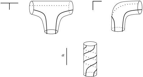
Figure 2. Local types for the link carried by a trellis. The vertical tube carries $a\in{\mathbb{Z}}$ half-twists ($a=3$ is pictured).

4.1. Nice flypeable trellises

Every maximal connected union of horizontal edges of $\mathcal{T}$ is called a horizontal line. A trapezoidal region bounded by two horizontal lines and containing only vertical edges in its interior is called a horizontal layer.

A trellis is brick like of type $(b,c)$ if it is a union of $b$ layers each containing $c$ squares arranged in such a way so that:

1. Vertical edges incident to a horizontal line (except the top and bottom lines) point alternately up and down.

2. Layers are alternately “left protruding” and “right protruding”, where by left protruding we mean that the leftmost vertical edge is to the left of the leftmost vertical edges in the layers both above and below it. The definition for right protruding and for the top and bottom layers is done in the obvious way.

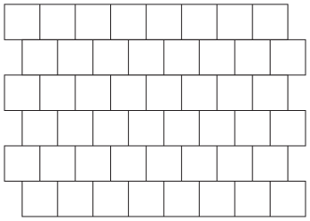
Figure 3. A brick-like trellis

A trellis is flypeable (see Figure 4) if it is obtained from a brick like trellis in the following way: Choose $1<i<b$, and in the $i-th$ layer choose a contiguous sequence of squares $D_{1},\dots D_{r}$ not including the leftmost or rightmost square. Now remove all vertical edges incident to the squares from the layers above and below. See Figure 4 for an example.

A trellis is nice flypeable if $2<i<b-1$ and the squares $D_{1},\dots D_{r}$ do not include the two leftmost or the two rightmost squares.

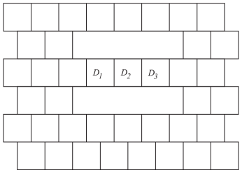
Figure 4. A nice flypeable trellis

Given a flypeable trellis carrying a knot or link $K$, a flype is an ambient isotopy of $K$ which is obtained as follows: Let $R$ be the union of the squares $D_{1},\dots D_{r}$ including their interiors. We call $R$ the flype rectangle. Let $B$ be a regular neighborhood of $R$. We choose $B$ so that it contains all subarcs of $K$ winding around the edges of $R$ except for the horizontal arcs of $K$ that travel in the back of $\Sigma$ along the horizontal edges of $R$. Hence $\partial B$ intersects $K$ in four points (see Figure 5.)

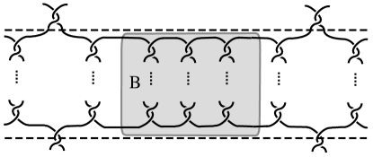
Figure 5. The box $B$ contains a portion of the knot associated to adjacent vertical edges, but excludes the horizontal arcs passing in the back (dotted).

A flype will flip the box $B$ by 180 degrees about a horizontal axis leaving all parts of the knot outside a small neighborhood of $B$ fixed. This operation changes the projection of $K$ in $P$ by adding a crossing on the left and a crossing on the right side of the box. These crossings have opposite signs.

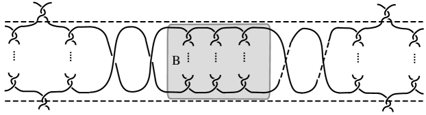
Figure 6. Local picture of $K^{2}$, a double-flype move on $K$. Note that the genus of the new trellis which carries $K^{2}$ is bigger by 4 than the genus of the trellis which carried $K$.

The projection of $K$ obtained after a flype is carried by a new trellis. It differs from $\mathcal{T}$ in that there is a new vertical edge on the left side of $R$ and another new one on the right side of $R$, one with twist coefficient $1$ and the other one with $-1$. The flype will be called positive if the coefficient of the left new edge is positive. A positive / negative flype iterated $|\,r\,|$ times will be called a $r$-flype, $r\in\mathbb{Z}$, (see Figure 6). Denote the image of $K$ after the $r$-flype by $K^{r}$ and the new trellis with the new $2|r|$ vertical edges by $\mathcal{T}^{r}$. Similarly we will denote $\operatorname{\mathcal{N}}(\mathcal{T}^{r})$ by $H_{1}^{r}$ and $\partial H_{1}^{r}$ by $\Sigma^{r}$. Notice that $g(\mathcal{T}^{r})=g(\mathcal{T})+2|r|$.

The following restatement of Theorem 3.4 of [12] describes the embedding of $K^{r}$ in $\Sigma^{r}$ under suitable assumptions:

Theorem 4.1.

Let $\mathcal{T}$ be a flypeable trellis and let $K=K[a]\subset S^{3}$ be a knot or link carried by $\mathcal{T}$ with twist coefficients given by $a$. Assume that $a(f)\geq 3$ for all vertical edges $f$ and that for the two vertical edges $e,e^{\prime}$ immediately to the left and right of the flype rectangle we have $a(e),a(e^{\prime})\geq 4$. Then for all $r\in\mathbb{Z}$, the surface $\Sigma^{r}\smallsetminus K^{r}[a]$ is incompressible in both the interior and the exterior handlebodies $H_{1}^{r},H_{2}^{r}$.

4.2. Horizontal surgery on knots carried by a trellis

In our construction we will need $K$ to be a knot. The number of components of $K$ is determined by the residues $a(e)\mod 2$, and it is easy to see that if $K$ has more than one component then the number can be reduced by changing $a(e)\mod 2$ at a column where two components meet. Hence a given trellis always carries knots with arbitrarily high coefficients. We will assume from now on that $K$ is a knot.

The embedding of $K$ in $\Sigma$ defines a framing, in which the longitude $\lambda_{\Sigma}$ is a boundary component of a regular neighborhood of $K$ in $\Sigma$. We let $K_{\Sigma}(p/q)$ denote the result of $p/q$ surgery on $S^{3}\smallsetminus K$ with respect to this framing.

In particular $K_{\Sigma}(1/m)$, for $m\in\mathbb{Z}$, will be called a horizontal Dehn surgery on $K$ with respect to $\Sigma$. Note that it has the same effect as cutting $S^{3}$ open along $\Sigma$ and regluing by the $m^{th}$ power of a Dehn twist on $K$.

It is interesting to note that a flype does not change this framing, i.e.

$$K_{\Sigma}(p/q)=K^{r}_{\Sigma^{r}}(p/q)$$

for all $p/q$ (see [12]). This is because the effects on the framing from the new crossings on both sides of the flypebox cancel each other out. We will not, however, need this fact in our construction.

5. Satisfying conditions for primitive stability

In this section we will consider representations for manifolds obtained from diagrams of flyped knots on a nice flypeable trellis. We show that they are hyperbolic and that they satisfy the hypotheses required by Proposition 3.5.

5.1. Whitehead graph

Fix $r\in\mathbb{Z}$. Let $\{e_{1},\dots,e_{n_{r}}\}$ denote the set of vertical edges of $\mathcal{T}^{r}$ not including the rightmost one in each layer. Each $e_{i}$ is dual to a disk $\Delta_{i}$ in $H_{1}^{r}$, and note that these disks cut $H^{r}_{1}$ into a 3-ball, hence $n_{r}=g(H^{r}_{1})$. Let $x_{i}$ be the generator of $\pi_{1}(H^{r}_{1})=F_{n_{r}}$ which is dual to $\Delta_{i}$ and let $X=\{x_{1},\ldots,x_{n_{r}}\}$. The curve $K^{r}$ contains no arc that meets a disk $\Delta_{i}$ from the same side at each endpoint without meeting other $\Delta_{j}$ in its interior, and it follows that $K^{r}$ determines a cyclically reduced word $[K^{r}]$ in the generators $X$.

Lemma 5.1.

The Whitehead graph $Wh([K^{r}],X)$ is cut point free for each $r\in\mathbb{Z}$.

Proof.

A regular neighborhood of each $\Delta_{i}$ in $H^{r}_{1}$ is bounded by two disks $\Delta_{i}^{\pm}$. Let $Q$ denote $H^{r}_{1}$ minus these regular neighborhoods. Then $K^{r}\cap Q$ is a collection of arcs corresponding to the edges of the Whitehead graph, and the disks $\Delta_{i}^{\pm}$ represent the vertices. After collapsing each disk to a point we get the Whitehead graph itself. Since $K^{r}$ meets each $\Delta_{i}$ in exactly two points, this graph is necessarily a 1-manifold. Now we observe that one can isotope this 1-manifold in a neighborhood of each horizontal line of the trellis so that the vertical coordinate of the plane $P$ is a height function on it with exactly one minimum and one maximum. Hence it is a circle, and in particular cut point free.

∎

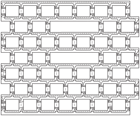
Figure 7. A representative nice flypeable trellis carrying a knot.

5.2. Hyperbolicity

Next we prove the hyperbolicity of our knot complements:

Theorem 5.2.

Let $\mathcal{T}$ be a nice flypeable trellis and let $K=K[a]\subset S^{3}$ be a knot or link carried by $\mathcal{T}$. Assume that $a(f)\geq 3$ for all vertical edges $f$. Assume further that the pair of edges $(e,e^{\prime})$ at the sides of the flype region have twist coefficients $a(e),a(e^{\prime})\geq 4$. Then $X=S^{3}\smallsetminus\operatorname{\mathcal{N}}(K)$ is a hyperbolic manifold.

Note that this gives us hyperbolicity of $S^{3}\smallsetminus\mathcal{N}(K^{r})$ for all $r\in\mathbb{Z}$, since $\{K^{r}\}$ are all isotopic.

Proof.

Recall that $H_{1}$ and $H_{2}$ are the interior and exterior handlebodies, respectively, of the trellis on which $K$ is defined. We first reduce the theorem to statements about annuli in $H_{2}$:

Lemma 5.3.

If the pared manifold $(H_{2},\overline{\mathcal{N}}_{\Sigma}(K))$ is acylindrical, then $X$ has no essential tori.

Proof.

Let $T\subset X$ be an incompressible torus, and let us prove that it is boundary-parallel. Choose $T$ to intersect the surface $\Sigma\smallsetminus\operatorname{\mathcal{N}}(K)$ transversally and with a minimal number of components.

The intersection $T\cap(\Sigma\smallsetminus\operatorname{\mathcal{N}}(K))$ must be non-empty since handlebodies do not contain incompressible tori. Since $K$ satisfies the conditions of Proposition 4.1, the surface $\Sigma\smallsetminus\operatorname{\mathcal{N}}(K)$ is incompressible in both the inner and outer handlebodies $H_{1}$ and $H_{2}$.

The intersection $T\cap\Sigma$ cannot contain essential curves in $\Sigma\smallsetminus\operatorname{\mathcal{N}}(K)$ which are inessential in $T$ and essential curves in $T$ which are inessential in $\Sigma\smallsetminus\operatorname{\mathcal{N}}(K)$ as this would violate the fact that both surfaces are incompressible. Curves that are inessential in both surfaces are ruled out by minimality. Hence $T\cap H_{i}$ ($i=1,2$) is a collection of essential annuli in $T$ which are incompressible in $H_{i}\smallsetminus\mathcal{N}(K)$. By minimality they are not parallel to $\partial H_{i}\smallsetminus\mathcal{N}(K)$.

By the hypothesis of the lemma, $T\cap H_{2}$ is a union of concentric annuli parallel to a neighborhood of $K$ in $\partial H_{2}$.

Suppose first that there is a single such annulus $A$. If we push $A$ to a component $A_{1}$ of a neighborhood of $K$ in $\partial H_{2}$, we obtain a torus $T^{\prime}$ in $H_{1}$ which is homotopically nontrivial, and hence bounds a solid torus $V$ in $H_{1}$. The intersection $V\cap\partial H_{1}$ is $A_{1}$. If $A_{1}$ is a primitive annulus in $V$ then so is its complement, which is just $T^{\prime}\cap H_{1}=T\cap H_{1}$. Hence $T\cap H_{1}$ is boundary parallel to $A_{1}$, so $T$ is an inessential torus in $M_{\infty}$, and we are done.

If $A_{1}$ is not primitive in $V$, then we have exhibited the handlebody $H_{1}$ as a union $V\cup W$, where $W$ is a handlebody of genus greater than one and $W\cap V$ is an annulus $A_{2}$ in $\partial W$. Now $A_{2}$ cannot be primitive in $W$, since $\partial W\smallsetminus A_{2}=\Sigma\smallsetminus A_{1}$, which is incompressible. But the gluing of two handlebodies along an annulus produces a handlebody only if the annulus is primitive to at least one side. (This follows from the fact that any annulus in a handlebody has a boundary compression, which determines a disk on one side intersecting the core of the annulus in a single point.) This is a contradiction.

Now if $T\cap H_{2}$ consists of more than one annulus, then one of the annuli, together with a neighborhood of $K$, bounds a solid torus $U$ in $H_{2}$ which contains all of the other annuli. Naming the annuli $B_{1},\ldots B_{n}$, where $B_{1}$ is the outermost, let $U^{\prime}$ denote $U$ minus a regular neighborhood of $B_{1}$, so that $U^{\prime}$ contains $B_{2}\cup\cdots\cup B_{n}$, and let $H^{\prime}_{1}=H_{1}\cup U^{\prime}$. We can isotope $K$ through $U^{\prime}$ to a knot $K^{\prime}$ on $\partial H^{\prime}_{1}$, so that the isotopy intersects $T$ in a disjoint union of cores of $B_{2},\ldots,B_{n}$. Now $H^{\prime}_{2}=cl(M\smallsetminus H^{\prime}_{1})$ intersects $T$ in the single annulus $B_{2}$, and we can apply the previous argument to show that $T$ bounds a solid torus $V$ in which $K^{\prime}$ is primitive. If $n$ is even, then $K$ is outside $V$, so that $T$ is inessential already. If $n$ is odd then $K$ is inside $V$, and since the isotopy from $K$ to $K^{\prime}$ passed through a sequence of disjoint curves in $T$, we conclude that $K$ is itself primitive in $V$. Hence again $T$ is inessential.

∎

Proposition 5.4.

Let $K$ be a knot carried by a nice flypeable trellis so that $a(e)\geq 3$ for every vertical edge $e$. Then there are no essential annuli in $(H_{2},\mathcal{N}_{\Sigma}(K))$.

Before we prove this proposition we need some definitions and notation. The proof will be somewhat technical and enumerative, but the notation and data we will set up will then be useful in proving Proposition 5.10 which applies to the flyped case.

Denote by $\mathcal{D}$ the collection of disks in $P$ which are the bounded regions of $P\smallsetminus\mathcal{N}_{P}(\mathcal{T})$. The front side of each $D\in\mathcal{D}$ will be denoted by $D^{+}$ and the back side by $D^{-}$. Set $\widehat{\mathcal{D}}=\{D^{+},D^{-}\,:\,D\in\mathcal{D}\}$, the set of “disk sides”. The number of vertical edges of $\mathcal{T}$ adjacent to the top (resp. bottom) edge of a disk $D$ is denoted by $tv(D)$ (resp. $bv(D)$). Each $D\in\mathcal{D}$ is contained in a single component of $P\smallsetminus\mathcal{T}$, and we sometimes abuse notation by calling this larger disk $D$ as well.

Proof of Proposition 5.4.

Assume that $A$ is a properly embedded incompressible annulus in $(H_{2},\overline{\mathcal{N}}_{\Sigma}(K))$ which is not parallel to $\partial H_{2}\smallsetminus\mathcal{N}(K)$. We will show that it is parallel to a neighborhood of $K$ in $\partial H_{2}$ and hence not essential.

The proof will be in two stages. In the first step we will show that, after isotopy, any such annulus $A$ can be decomposed as a cycle of rectangles where two adjacent rectangles meet along an arc of intersection of $A$ with $\mathcal{D}$. In the second step we show that a cycle of rectangles must be parallel to the knot. Throughout we will abuse notation by referring to $\cup_{D\in\mathcal{D}}D$ as just $\mathcal{D}$.

Step 1: The disks of $\mathcal{D}$ are essential disks in the outer handlebody $H_{2}$, and $H_{2}\smallsetminus\operatorname{\mathcal{N}}(\mathcal{D})$ is a $3$-ball. Note that the disk-sides in $\widehat{\mathcal{D}}$ can be identified with disks of $\partial\operatorname{\mathcal{N}}(\mathcal{D})$ that lie in the boundary of this ball. Isotope $A$ to intersect $\mathcal{D}$ transversally and with a minimal number of components. The intersection must be nonempty, as otherwise $A$ will be contained in a $3$-ball and will not be essential. No component of $A\cap\mathcal{D}$ can be a simple closed curve, since this would either violate the the fact that $A$ is essential, or allow us to reduce the number of components in $A\cap\mathcal{D}$ by cutting and pasting.

Let $\mathcal{E}$ denote the set of components of $\Sigma\smallsetminus(K\cup\mathcal{D})$. By Lemma 2.2 of [12] we have that each $E\in\mathcal{E}$ is a 2-cell, and that the intersection of $\partial E$ with any disk $D\in\mathcal{D}$ is either

1. empty or

2. consists of precisely one arc or

3. consists of precisely two arcs along which $E$ meets $\mathcal{D}$ from opposite sides of $P$.

(One can also obtain these facts from the enumeration that we will shortly describe of all local configurations of $\mathcal{E}$, and in fact we will generalize this later).

We claim the arcs of intersection in $A\cap\mathcal{D}$ must be essential in $A$: If not, consider an outermost such arc $\delta$ which, together with a subarc $\alpha\subset\partial A$, bounds a sub-disk $\Delta_{1}$ in $A$. Let $D$ be the component of $\mathcal{D}$ containing $\delta$. By transversality, a neighborhood of $\delta$ in $\Delta_{1}$ exits $P$ from only one side, and hence both ends of $\alpha$ meet $\delta$ from the same side of $P$. The arc $\alpha$ is contained in a single component $E$ of $\Sigma\smallsetminus(K\cup\mathcal{D})$. If $\partial E$ meets $D$ in more than one arc then, by (3) above, it does so from opposite sides of $P$. Hence the endpoints of $\alpha$ can meet only one such arc in $\partial E$. Since $E$ is a polygon, $\alpha$ together with a subarc $\gamma$ of $\partial D\cap\partial E$ bound a sub-disk $\Delta_{2}\subset E$. Now $\gamma$ and $\delta$ must bound a sub-disk $\Delta_{3}$ in $D$. The union $\Delta_{1}\cup\Delta_{2}\cup\Delta_{3}$ is a $2$-sphere in the complement of $K$ which bounds a $3$-ball in $X$. Hence we can isotope $A$ to reduce the number of components in $A\cap\mathcal{D}$ in contradiction to the choice of $A$. We conclude that all arcs of $A\cap\mathcal{D}$ are essential in $A$.

As the intersection arcs in $A\cap\mathcal{D}$ are essential in $A$ they cut it into rectangles. We can summarize this structure in the following lemma:

Lemma 5.5.

After proper isotopy in $(H_{2},\overline{\mathcal{N}}_{\Sigma}(K))$, an incompressible annulus $A$ intersects $\mathcal{D}$ in a set of essential arcs, which cut $A$ into rectangles. The boundary of a rectangle can be written as a union of arcs $\delta_{1},\delta_{2}\subset A\cap\mathcal{D}$, and arcs $\alpha_{1},\alpha_{2}\subset\partial A$, so that $\alpha_{1}$ and $\alpha_{2}$ are contained in distinct components $E_{1},E_{2}\in\mathcal{E}$.

What remains to prove is just the statement that the components $E_{1}$ and $E_{2}$ of $\mathcal{E}$ containing $\alpha_{1}$ and $\alpha_{2}$, respectively, are distinct.

Choose an arc $\delta$ of $A\cap\mathcal{D}$, and let $D$ be the disk in $\mathcal{D}$ containing $\delta$. We claim that $\partial\delta$ separates the points of $K\cap\partial D$ on $\partial D$. For if not, then $\delta$ would define a boundary compression disk for $A$ in $H_{2}$ which misses $K$. After boundary compressing $A$ we will obtain (since $A$ is not parallel to $\partial H_{2}\smallsetminus\mathcal{N}(K)$) an essential disk $\Delta\subset H_{2}$ with $\partial\Delta\subset\Sigma\smallsetminus\operatorname{\mathcal{N}}(K)$, which contradicts Proposition 4.1.

Now for a rectangle $R$ of $A\setminus\mathcal{D}$, since each $\delta_{i}$ in $\partial R$ separates $K\cap\partial D$ on $\partial D$, the arcs $\alpha_{1}$ and $\alpha_{2}$ meet $\partial D$ in different arcs of $\partial D\smallsetminus K$. Using transversality as before, $\alpha_{1}$ and $\alpha_{2}$ exit $D$ from the same side of $P$, and hence by properties (1-3) above (from Lemma 2.2 of [12]), they cannot be contained in the same component $E$ of $\mathcal{E}$. We conclude that $E_{1}\neq E_{2}$. This completes the proof of Lemma 5.5.

We will adopt the notation $(D^{e_{1}}_{1},D^{e_{2}}_{2},E_{1},E_{2})$ to describe the data that determine a rectangle up to isotopy, where $D^{e_{i}}_{i}\in\widehat{\mathcal{D}}$ and $E_{i}\in\mathcal{E}$. That is, the rectangle meets $D_{i}$ along its boundary arcs $\delta_{i}$ on the sides determined by $e_{i}$, and the arcs $\alpha_{i}$ are contained in $E_{i}$. We call a rectangle trivial if $E_{1}$ and $E_{2}$ are adjacent along a single sub-arc of $K\smallsetminus\mathcal{D}$. This is because the rectangle can then be isotoped into a regular neighborhood of this sub-arc.

Step 2: We now show that if $H_{2}=S^{3}\smallsetminus\mathcal{N}(\mathcal{T})$, where $\mathcal{T}$ is a nice flypeable trellis, one cannot embed in $\partial H_{2}\smallsetminus\operatorname{\mathcal{N}}(K)$ a sequence of non-trivial rectangles $R$, as above, which fit together to compose an essential annulus $A$.

We first prove the following lemma:

Lemma 5.6.

If $(D^{e_{1}}_{1},D^{e_{2}}_{2},E_{1},E_{2})$ determines a non-trivial rectangle then $D_{1},D_{2}$ are contained in a single layer of the trellis.

After this we will prove Lemma 5.7 which enumerates the types of nontrivial rectangles which do occur, and Lemma 5.9 which describes the ways in which rectangles can be adjacent along their intersections with $\mathcal{D}$. We will then be able to see that the adjacency graph of nontrivial rectangles contains no cycles, which will complete the proof of Proposition 5.4.

The proof will be achieved by a careful enumeration of how disk-sides in $\widehat{\mathcal{D}}$ are connected by regions in $\mathcal{E}$. We will examine each type of disk in $\mathcal{D}$ on a case by case basis. For each disk we will consider only its connection to disks along $\mathcal{E}$ regions meeting it on the top and sides. The complete picture can be obtained using the fact that a $180$ rotation in $P$ of a nice flypeable trellis is also a nice flypeable trellis (see Figure 7).

Proof of Lemma 5.6.

We use the following notation:

1. Connectivity: The symbol

   $$D^{\pm}\stackrel{{\scriptstyle E}}{{\longleftrightarrow}}D^{\pm}_{1},\dots,D^{\pm}_{n}$$

   where $D^{\pm},D^{\pm}_{1},\dots,D^{\pm}_{n}\in\widehat{\mathcal{D}}$ and $E\in\mathcal{E}$, means that $E$ meets the disks $D,D_{1},\dots,D_{n}$ on the indicated sides. (Although the asymmetry of treating one disk differently from the others seems artificial here, it is suited to the order in which we enumerate cases).

2. Disk coordinates: When considering a given disk $D$ we will use relative “cartesian” coordinates $D_{i,j}$ for $D$ and its neighbors, where $D=D_{0,0}$, $i$ indicates layer and $j$ enumerates disks in a layer from left to right.

3. $\mathcal{E}$ region coordinates: The $\mathcal{E}$ region adjacent to the top edge of a disk will always be enumerated by $E_{0}$. Regions along the left and right edges will be enumerated in a clockwise direction by consecutive integers. Note that we do not enumerate the regions near the bottom of a disk and they can be understood by symmetry.

First we enumerate adjacencies for “front” disks $D^{+}$. In each case we will give a precise figure for the local configuration and a list of connectivity data which can be verified by inspection.

Middle disks

Begin with disks which are not leftmost or rightmost in their layer. Cases will be separated depending on the top valency of the disk in question.

1. $tv(D)=1$. The neighborhood of the top edge of $D=D_{0,0}$ is described in Figure 8.

   

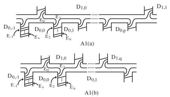
   Figure 8. This figure describes the case discussed in A1(a) and A1(b).

   Note that there are two cases, depending on whether $tv(D_{0,1})$ is zero or not.

   1. $tv(D_{0,1})=0$:

      $$D^{+}_{0,0} \stackrel{{\scriptstyle E_{0}}}{{\longleftrightarrow}}D_{1,0}^{+},D_{0,-1}^{+}$$

      $$D^{+}_{0,0} \stackrel{{\scriptstyle E_{1}}}{{\longleftrightarrow}}D_{1,0}^{+},D_{0,1}^{+},\dots,D^{+}_{0,p},D^{+}_{1,1}$$

      $$D^{+}_{0,0} \stackrel{{\scriptstyle E_{j}}}{{\longleftrightarrow}}D_{0,1}^{+},\,\,2\leq j\leq u$$

      $$D^{+}_{0,0} \stackrel{{\scriptstyle E_{k}}}{{\longleftrightarrow}}D_{0,-1}^{+},\,\,\,v\leq k\leq-1$$

   2. $tv(D_{0,1})>0$:

      $$D^{+}_{0,0} \stackrel{{\scriptstyle E_{0}}}{{\longleftrightarrow}}D_{1,0}^{+},D_{0,-1}^{+}$$

      $$D^{+}_{0,0} \stackrel{{\scriptstyle E_{1}}}{{\longleftrightarrow}}D_{1,0}^{+},D_{1,1}^{+}$$

      $$D^{+}_{0,0} \stackrel{{\scriptstyle E_{2}}}{{\longleftrightarrow}}D_{0,1}^{+},D_{1,1}^{+},\dots,D^{+}_{1,q}$$

      $$D^{+}_{0,0} \stackrel{{\scriptstyle E_{j}}}{{\longleftrightarrow}}D_{0,1}^{+},\,\,\,3\leq j\leq u$$

      $$D^{+}_{0,0} \stackrel{{\scriptstyle E_{k}}}{{\longleftrightarrow}}D_{0,-1}^{+},\,\,\,v\leq k\leq-1$$

2. $tv(D)>1$ (see Figure 9). Note that $D_{1,s}$ is not the rightmost disk in its layer, by the nice flypeable condition.

   $$D^{+}_{0,0} \stackrel{{\scriptstyle E_{0}}}{{\longleftrightarrow}}D_{1,0}^{+},\dots,D^{+}_{1,s},D_{0,-1}^{+}$$

   $$D^{+}_{0,0} \stackrel{{\scriptstyle E_{1}}}{{\longleftrightarrow}}D_{1,s}^{+},D_{1,s+1}^{+}$$

   $$D^{+}_{0,0} \stackrel{{\scriptstyle E_{2}}}{{\longleftrightarrow}}D_{1,s+1}^{+},D_{0,1}^{+}$$

   $$D^{+}_{0,0} \stackrel{{\scriptstyle E_{j}}}{{\longleftrightarrow}}D_{0,1}^{+},\,\,\,3\leq j\leq u$$

   $$D^{+}_{0,0} \stackrel{{\scriptstyle E_{k}}}{{\longleftrightarrow}}D_{0,-1}^{+},\,\,\,v\leq k\leq-1$$

   

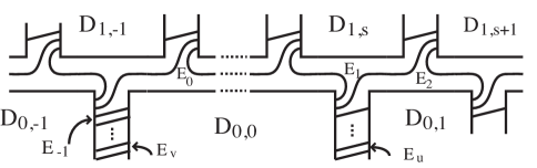
   Figure 9. The case where $tv(D)>1$, discussed in A2.

3. $tv(D)=0$.

   1. $D$ is not in the top row (see Figure 10). In this case $D$ can be one of a sequence $D_{0,s},\dots,D_{0,0},\dots,D_{0,t},\,\,(s\leq 0\leq t)$ of disks whose top edge is adjacent to the bottom edge of $D_{1,0}$. If it is not the rightmost one in the sequence (i.e. $t>0$) then:

      $$D^{+}_{0,0} \stackrel{{\scriptstyle E_{0}}}{{\longleftrightarrow}}D_{0,-1}^{+}$$

      $$D^{+}_{0,0} \stackrel{{\scriptstyle E_{1}}}{{\longleftrightarrow}}D_{1,0}^{+},D_{1,1}^{+},D^{+}_{0,s-1},D^{+}_{0,s},\dots,D^{+}_{0,t}$$

      $$D^{+}_{0,0} \stackrel{{\scriptstyle E_{2}}}{{\longleftrightarrow}}D_{0,1}^{+}$$

      $$D^{+}_{0,0} \stackrel{{\scriptstyle E_{j}}}{{\longleftrightarrow}}D_{0,1}^{+},\,\,\,3\leq j\leq u$$

      $$D^{+}_{0,0} \stackrel{{\scriptstyle E_{k}}}{{\longleftrightarrow}}D_{0,-1}^{+},\,\,\,v\leq k\leq-1$$

      If $D$ is the rightmost disk in the sequence (i.e. $t=0$) then replace

      $$D^{+}_{0,0}\stackrel{{\scriptstyle E_{2}}}{{\longleftrightarrow}}D_{0,1}^{+}$$

      by

      $$D^{+}_{0,0}\stackrel{{\scriptstyle E_{2}}}{{\longleftrightarrow}}D_{0,1}^{+},D_{1,1}^{+}$$

      

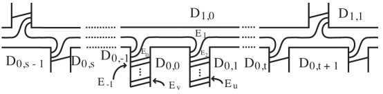
      Figure 10. The case where $tv(D)=0$, discussed in A3(a).

   2. If $D$ is in the top row (see Figure 11) then the region $E_{1}$ connects $D_{0,0}^{+}$ to all disks in the layer as well as to the back of the leftmost disk:

      $$D^{+}_{0,0}\stackrel{{\scriptstyle E_{1}}}{{\longleftrightarrow}}D_{0,s}^{-},D_{0,s}^{+},\dots,D_{0,t}^{+},$$

      where $s<0<t$ and $t-s+1=c$. The other connections are the same as in case $(a)$.

      

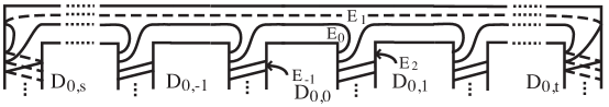
      Figure 11. The case where $tv(D)=0$, discussed in A3(b).

Edge disks

We now consider disks which are either leftmost or rightmost in their layer.

1. Let $D_{0,0}$ be the right disk in the top layer. This case is as in case A3(b) except that we set $t=0$. The region $E_{2}$ now connects $D^{+}_{0,0}$ to the back side $D_{0,i}^{-}$ of all disks in the top layer, and we replace

   $$D^{+}_{0,0}\stackrel{{\scriptstyle E_{j}}}{{\longleftrightarrow}}D_{0,1}^{+},\,\,\,3\leq j\leq u$$

   by

   $$D^{+}_{0,0}\stackrel{{\scriptstyle E_{j}}}{{\longleftrightarrow}}D_{0,0}^{-},\,\,\,3\leq j\leq u$$

2. Let $D_{0,0}$ be the left disk in a top layer.

   This case is as in case A3(b) except that we set $s=0$. Now $E_{k},\,v\leq k\leq 0$, connects $D^{+}_{0,0}$ to $D^{-}_{0,0}$.

   The following cases do not occur in top or bottom layers.

3. Let $D_{0,0}$ be the rightmost disk in a layer protruding to the left (see Figure 12).

   $$D^{+}_{0,0} \stackrel{{\scriptstyle E_{0}}}{{\longleftrightarrow}}D_{0,-1}^{+},D_{1,0}^{+}$$

   $$D^{+}_{0,0} \stackrel{{\scriptstyle E_{1}}}{{\longleftrightarrow}}D_{1,0}^{+},D_{1,0}^{-}$$

   $$D^{+}_{0,0} \stackrel{{\scriptstyle E_{2}}}{{\longleftrightarrow}}D_{1,0}^{-},D_{0,s}^{-},\dots,D_{0,0}^{-}$$

   $$D^{+}_{0,0} \stackrel{{\scriptstyle E_{j}}}{{\longleftrightarrow}}D_{0,0}^{-},\,\,\,3\leq j\leq u$$

   $$D^{+}_{0,0} \stackrel{{\scriptstyle E_{k}}}{{\longleftrightarrow}}D_{0,-1}^{+},\,\,\,v\leq k\leq-1$$

   where $D_{0,s}$ is the leftmost disk in the layer.

   

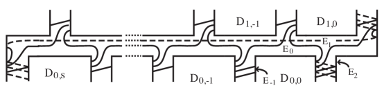
   Figure 12. Rightmost disk in layer protruding to the left as discussed in A6.

4. Let $D_{0,0}$ be the leftmost disk in a layer protruding to the left (see Figure 13).

   $$D^{+}_{0,0} \stackrel{{\scriptstyle E_{0}}}{{\longleftrightarrow}}D_{0,0}^{-},D_{1,0}^{+}$$

   $$D^{+}_{0,0} \stackrel{{\scriptstyle E_{1}}}{{\longleftrightarrow}}D_{1,0}^{+},D_{1,1}^{+}$$

   $$D^{+}_{0,0} \stackrel{{\scriptstyle E_{2}}}{{\longleftrightarrow}}D_{0,1}^{+},D_{1,1}^{+}$$

   $$D^{+}_{0,0} \stackrel{{\scriptstyle E_{j}}}{{\longleftrightarrow}}D_{0,1}^{+},\,\,\,3\leq j\leq u$$

   $$D^{+}_{0,0} \stackrel{{\scriptstyle E_{k}}}{{\longleftrightarrow}}D_{0,0}^{-},\,\,\,v\leq k\leq-1$$

   Note that $tv(D_{0,1})=1$ since we have a nice flypeable trellis.

   

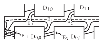
   Figure 13. Leftmost disk in layer protruding to the left as discussed in A7.

5. Let $D_{0,0}$ be the rightmost disk in a layer protruding to the right (see Figure 14).

   $$D^{+}_{0,0} \stackrel{{\scriptstyle E_{0}}}{{\longleftrightarrow}}D_{1,-1}^{-},D_{0,-1}^{+}$$

   $$D^{+}_{0,0} \stackrel{{\scriptstyle E_{1}}}{{\longleftrightarrow}}D_{1,t}^{+},D_{1,t}^{-},\dots,D_{1,-1}^{-}$$

   $$D^{+}_{0,0} \stackrel{{\scriptstyle E_{2}}}{{\longleftrightarrow}}D_{0,s}^{-},\dots,D_{0,0}^{-},D_{1,t}^{+}$$

   $$D^{+}_{0,0} \stackrel{{\scriptstyle E_{j}}}{{\longleftrightarrow}}D_{0,0}^{-},\,\,\,3\leq j\leq u$$

   $$D^{+}_{0,0} \stackrel{{\scriptstyle E_{k}}}{{\longleftrightarrow}}D_{0,-1}^{+},\,\,\,v\leq k\leq-1$$

   where $D_{0,s}$ and $D_{1,t}$ are the leftmost disks in their layers.

   

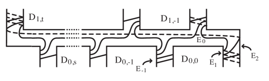
   Figure 14. Rightmost disk in layer protruding to the right as discussed in A8.

6. Let $D_{0,0}$ be the leftmost disk in a layer protruding to the right (see Figure 15).

   Note that $tv(D_{0,1})=1$ as we have a nice flypeable trellis.

   $$D^{+}_{0,0} \stackrel{{\scriptstyle E_{0}}}{{\longleftrightarrow}}D_{0,0}^{-},D_{1,0}^{+}$$

   $$D^{+}_{0,0} \stackrel{{\scriptstyle E_{1}}}{{\longleftrightarrow}}D_{1,0}^{+},D_{1,1}^{+}$$

   $$D^{+}_{0,0} \stackrel{{\scriptstyle E_{2}}}{{\longleftrightarrow}}D_{0,1}^{+},D_{1,1}^{+}$$

   $$D^{+}_{0,0} \stackrel{{\scriptstyle E_{j}}}{{\longleftrightarrow}}D_{0,1}^{+},\,\,\,3\leq j\leq u$$

   $$D^{+}_{0,0} \stackrel{{\scriptstyle E_{k}}}{{\longleftrightarrow}}D_{0,0}^{-},\,\,\,v\leq k\leq-1$$

   

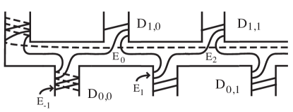
   Figure 15. Leftmost disk in layer protruding to the right as discussed in A9.

Now consider disks of type $D^{-}$ (see Figure 16):

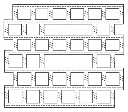
Figure 16. Configuration on the back of $H_{1}$. The sub-arcs of the knot are indicated by the dashed arcs.

In the back of each layer there are two “long” regions $F$ and $F^{\prime}$ which meet every back disk in its top or bottom edge respectively. In addition, in every interior column there is a sequence of regions which meet only the two adjacent disks to the column. The regions that meet the leftmost or rightmost columns (including $F$ and $F^{\prime}$) give connections from back disks to front disks in the same or adjacent layers. These connections were given in the discussion of the front disks.

The cases described above, together with their $180^{\circ}$ rotations, give all possible connections between disks. For example, the connections along the bottoms of the disks in cases (A4) and (A5) are obtained as rotations of the connections in cases (A6–A9).

It can now be checked that any time two $\mathcal{E}$ regions connect disks which are not in the same layer then these regions are adjacent along a single arc of $K\smallsetminus\mathcal{D}$. Here are some examples of this analysis:

In case (A1)(a) the only connections between $D^{+}_{0,0}$ and disks in a different row are

$$D^{+}_{0,0} \stackrel{{\scriptstyle E_{0}}}{{\longleftrightarrow}}D_{1,0}^{+}$$

$$D^{+}_{0,0} \stackrel{{\scriptstyle E_{1}}}{{\longleftrightarrow}}D_{1,0}^{+}\,\,\,and$$

$$D^{+}_{0,0} \stackrel{{\scriptstyle E_{1}}}{{\longleftrightarrow}}D^{+}_{1,1}$$

Note that $E_{0}$ and $E_{1}$ are adjacent along a single arc and hence the rectangle determined by the first two lines is trivial.

In case (A2) the only connections between $D^{+}_{0,0}$ and disks in a different row are:

$$D^{+}_{0,0} \stackrel{{\scriptstyle E_{0}}}{{\longleftrightarrow}}D_{1,0}^{+},\ldots,D_{1,s-1}^{+}$$

$$D^{+}_{0,0} \stackrel{{\scriptstyle E_{0}}}{{\longleftrightarrow}}D_{1,s}^{+}$$

$$D^{+}_{0,0} \stackrel{{\scriptstyle E_{1}}}{{\longleftrightarrow}}D_{1,s}^{+}$$

$$D^{+}_{0,0} \stackrel{{\scriptstyle E_{1}}}{{\longleftrightarrow}}D^{+}_{1,s+1}$$

$$D^{+}_{0,0} \stackrel{{\scriptstyle E_{2}}}{{\longleftrightarrow}}D^{+}_{1,s+1}$$

Here the connections in the first line do not belong to any rectangle. The second and third line define a trivial rectangle, and so do the third and fourth.

In case (A7) the only connections between $D^{+}_{0,0}$ and disks in a different row are:

$$D^{+}_{0,0} \stackrel{{\scriptstyle E_{0}}}{{\longleftrightarrow}}D_{1,0}^{+}$$

$$D^{+}_{0,0} \stackrel{{\scriptstyle E_{1}}}{{\longleftrightarrow}}D_{1,0}^{+}$$

$$D^{+}_{0,0} \stackrel{{\scriptstyle E_{1}}}{{\longleftrightarrow}}D^{+}_{1,1}$$

$$D^{+}_{0,0} \stackrel{{\scriptstyle E_{2}}}{{\longleftrightarrow}}D^{+}_{1,1}$$

Here the first and second lines define a trivial rectangle as do the third and fourth.

Finally, let $D^{-}$ be a back disk in the middle of a layer protruding to the left. It is connected to the the rightmost front disk of the layer below using the connections in (A8) second line, and to the rightmost back disk of the layer above using the connections in (A6) third line. None of these connections is part of a rectangle.

The remaining cases are similar (for the global picture it is helpful to consult Figure 7), and an inspection of them completes the proof of the lemma.

∎

We now compile a list of the nontrivial rectangles. First we list nontrivial rectangles from front disks to front disks.

1. Disks which share a vertical column $e$ (see Figure 17). The disks will be numbered $D_{0,0}$ and $D_{0,1}$. The $\mathcal{E}$ regions will be numbered clockwise around $D_{0,0}$ starting from the top.

   1. $tv(D_{0,1})>0$, $bv(D_{0,0})>0$:

      We obtain a rectangle for ($D^{+}_{0,0},D^{+}_{0,1},E_{i},E_{j}$),

      where $2\leq i<j\leq a(e)$.

   2. $tv(D_{0,1})=0$, $bv(D_{0,0})=0$:

      We obtain a rectangle for ($D^{+}_{0,0},D^{+}_{0,1},E_{i},E_{j}$),

      where $1\leq i<j\leq a(e)+1$.

   3. $tv(D_{0,1})=0$, $bv(D_{0,0})>0$:

      We obtain a rectangle for ($D^{+}_{0,0},D^{+}_{0,1},E_{i},E_{j}$),

      where $1\leq i<j\leq a(e)$.

   4. $tv(D_{0,1})>0$, $bv(D_{0,0})=0$:

      This case is obtained from the previous one by a $180^{\circ}$ rotation.

   In all preceding cases the rectangles are nontrivial when $j-i\geq 2$.

   

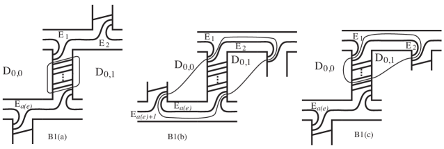
   Figure 17. Case B1. For each subcase one example rectangle is indicated by a simple closed curve tracing out its boundary. In (a), $(i,j)=(2,a(e))$. In (b), $(i,j)=(1,a(e)+1)$. In (c), $(i,j)=(1,a(e)-2)$.

2. Consider a sequence of disks in a layer which is contained in a flype box or is in a top or bottom layer which is adjacent to a flype box. In such cases we obtain a sequence $D_{0,0},\dots,D_{0,p}$ so that

   $$tv(D_{0,k})=0,\,1\leq k\leq p,$$

   $$bv(D_{0,k})=0,\,0\leq k\leq p-1$$

   We obtain a nontrivial rectangle ($D^{+}_{0,0},D^{+}_{0,p},E_{1},E_{-1}$). Note that the case $p=1$ already appears in case (B1).

   

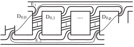
   Figure 18. Case B2.

We now consider rectangles which connect back disks to back disks. The back of every layer has the same structure, which can be seen in Figure 16: There are two “long” $\mathcal{E}$ regions denoted by $F,F^{\prime}$, which meet every disk on its top and bottom edge respectively. Given a column $e$ there is a sequence of at least two regions which connect the disks adjacent to $e$, which we number $F_{1},\dots,F_{a(e)-1}$ from top to bottom.

1. For any two $D_{0,p},D_{0,q}$ in a layer there is a rectangle ($D^{-}_{0,p},D^{-}_{0,q},F,F^{\prime}$).

2. Let $e$ be the column between $D_{0,p}$ and $D_{0,p+1}$, and $F_{1},\ldots,F_{a(e)-1}$ the associated regions. Moreover write $F_{0}=F$ and $F_{a(e)}=F^{\prime}$. These determine rectangles

   $$(D^{-}_{0,p},D^{-}_{0,p+1},F_{i},F_{j}),\,\,0\leq i<j\leq a(e)$$

   which are nontrivial when $j-i\geq 2$.

We now consider rectangles which connect front disks to back disks. These occur at the right and left edges of the trellis.

In $(B5-B10)$ let $D$ be a rightmost or leftmost disk in a layer, and let $e$ be the column to its right or left respectively. We number the regions meeting $D^{+}$ clockwise around $D$, with $E_{0}$ meeting the top edge. We then have the following rectangles, all of which can be seen in Figures 7 and 16:

1. Let $D$ be a rightmost disk in a left protruding inner layer. There are rectangles:

   $$(D^{+},D^{-},E_{i},E_{j}),\,\,2\leq i<j\leq a(e)$$

   Note that $D^{+}$ connects to the back of the first disk in the layer through only one region, hence there is no corresponding rectangle.

2. Let $D$ be a rightmost disk in a right protruding inner layer. There are rectangles:

   $$(D^{+},D^{-},E_{i},E_{j}),\,\,2\leq i<j\leq a(e)$$

3. Let $D$ be a rightmost disk in a right protruding bottom layer. There are rectangles:

   $$(D^{+},D^{-},E_{i},E_{j}),\,\,2\leq i<j\leq a(e)+1$$

   
   

4. Let $D$ be a leftmost disk in a right protruding bottom layer. There are rectangles:

   $$(D^{+},D^{-},E_{i},E_{j}),\,\,-a(e)+2\leq j<i\leq 0$$

5. Let $D$ be a leftmost disk in a right protruding top layer. There are rectangles:

   $$(D^{+},D^{-},E_{i},E_{j}),\,\,-a(e)+2\,\leq j<i\leq 1$$

6. Let $D$ be a rightmost disk in a right protruding top layer. There are rectangles:

   $$(D^{+},D^{-},E_{i},E_{j}),\,\,2\leq i<j\leq a(e)$$

All remaining cases are obtained from the above by a $180^{\circ}$ rotation of the plane $P$. The rectangles are non trivial when $j-i\geq 2$.

Lemma 5.7.

All nontrivial rectangles are described in cases $(B1)-(B10)$.

Proof.

By Lemma 5.6, we need to consider only rectangles between disks contained in a single horizontal layer. The proof is then a case by case inspection, using the same data and techniques as the proof of Lemma 5.6.

∎

Two rectangles $R=(D_{1}^{e_{1}},D_{2}^{e_{2}},E_{1},E_{2})$, and $R^{\prime}=(D_{3}^{e_{3}},D_{4}^{e_{4}},E_{3},E_{4})$, where $e_{i}\in\{\pm 1\},i=1\dots,4$, will be called adjacent along $D_{2}$ if the following holds:

1. $D_{2}=D_{3}$ and $e_{2}=-e_{3}$ and

2. The arcs of intersection $E_{1}\cap D_{2},E_{2}\cap D_{2}$ are equal to the arcs of intersection $E_{3}\cap D_{3},E_{4}\cap D_{3}$.

This condition captures the combinatorial aspects of an adjacency of rectangles in the annulus $A$.

If after renumbering $R$ and $R^{\prime}$ are adjacent along one of the disks, we say that they are adjacent.

Lemma 5.8.

There are no adjacencies between trivial and non trivial rectangles.

Proof.

An inspection of cases (B1 - B10) shows that given a non trivial rectangle $R=(D_{1}^{e_{1}},D_{2}^{e_{2}},E_{1},E_{2})$, the arcs of intersection $E_{1}\cap D_{i}$ and $E_{2}\cap D_{i}$ for each $i=1,2$ are separated by at least two points of $K\cap\partial D_{i}$. Since for a trivial rectangle these arcs are always separated by just one such point, there can be no adjacencies between trivial and nontrivial rectangles.

∎

The adjacency graph of rectangles will be the graph whose vertices are rectangles, where we place and edge between $R$ and $R^{\prime}$, labeled by $D$, whenever $R$ and $R^{\prime}$ are adjacent along $D$. Formally speaking a pair rectangles might have distinct adjacencies labeled by the same disk. However, the arguments in Lemma 5.9 show that this never occurs in our setting.

Lemma 5.9.

In the adjacency graph of rectangles, every cycle contains only trivial rectangles.

Proof.

By Lemma 5.8, if a cycle contains any trivial rectangle then it contains only trivial rectangles. Hence it suffices to restrict to the subgraph of nontrivial rectangles and show that it contains no cycles.

Wrapping around each vertical column there are (several) sequences of adjacent rectangles. Consider for example case (B1)(a). A front rectangle indexed by $(i,j),i\geq 3,$ is adjacent to a back rectangle from case (B4) indexed by $(i-2,j-2)$. If $i-2\geq 2$ then this rectangle is adjacent to a front rectangle indexed by $(i-2,j-2)$. If $i-2\leq 1$ there are no further adjacencies. Hence any such chain terminates in a rectangle that has no further adjacencies and thus is not part of a cycle.

Similar arguments apply to the rest of case (B1), with one proviso: If $tv(D_{0,1})=0$ and a back rectangle is indexed by $(1,j)$, then it is adjacent to one further front rectangle indexed by $(1,j)$ (see Figure 17 case (c)), but that rectangle meets $D_{0,1}$ in two vertical arcs on opposite edges. Any rectangle involving $D_{0,1}^{-}$ meets it either in vertical arcs on the same edge of $\partial D_{0,1}$ (cases (B4 - B10)), one vertical arc and one horizontal edge (case (B4)), or in horizontal edges (case (B3)). Hence the chain terminates at this point.

A front rectangle in case (B2) again meets its disks along vertical arcs on opposite edges, and so is not adjacent to any rectangle.

In cases (B5 - B10), a similar analysis as case (B1) holds. Note that in these cases rectangles are not divided into “front” and “back”, rather each rectangle wraps around from front to back.

Every adjacency of a back rectangle must be to a rectangle of type already discussed, hence back rectangles cannot be a part of a cycle either.

∎

Every essential annulus $A\subset(H_{2},\mathcal{N}(K))$ determines a cycle of rectangles in the adjacency graph, and Lemma 5.9 implies that all these rectangles are trivial. Hence the annulus is parallel to the knot. This finishes the proof of Proposition 5.4

∎

Lemma 5.3 together with Proposition 5.4 and Thurston’s Haken geometrization theorem complete the proof of Theorem 5.2.

∎

5.3. Ruling out $I$-bundles

In order to apply Proposition 3.5 to the proof of Theorem 1.1 we need to further show that $(H^{r}_{2},\overline{\mathcal{N}}_{\Sigma^{r}}(K^{r}))$ is not an $I$-bundle. We do this in the following lemma:

Proposition 5.10.

For each $r\in\mathbb{Z}$ the pared manifold $(H^{r}_{2},\overline{\mathcal{N}}_{\Sigma^{r}}(K^{r}))$ is not an $I$-bundle.

Proof.

For $r=0$ this is a consequence of Proposition 5.4. The rest of the proof will be given for $r>0$. The case $r<0$ will follow from the usual $180^{\circ}$ rotation.

In this case it is easy to see that $(H^{r}_{2},\mathcal{N}_{\Sigma^{r}}(K^{r}))$ does in fact contain essential annuli. In particular Lemma 5.8 fails because now there are columns with $a(e)=1$ and this allows adjacencies between trivial and nontrivial rectangles.

The idea is to prove that there is a union of (one or two) essential annuli in $(H^{r}_{2},\mathcal{N}_{\Sigma^{r}}(K^{r}))$ which separates $(H^{r}_{2},\mathcal{N}_{\Sigma^{r}}(K^{r}))$ into two components, one of which contains no essential annuli. This is impossible in an $I$-bundle, since an $I$-bundle does not have a non-trivial JSJ decomposition (see [8]) hence the proposition follows.

Consider the rectangular closed curve labeled $\tau$ in Figure 19. Let $\tau^{+}$ ($\tau^{-}$) denote the curve in the front (back) of $\Sigma$ lying in front of (back of) $\tau$. The curves $\tau^{+}$, $\tau^{-}$ bound disks denoted by $\Delta_{F}$ and $\Delta_{B}$ in $H_{2}^{r}$, whose projection to $P$ is the disk $\Delta$ bounded by $\tau$. The points between $\Delta_{F}$ and $\Delta_{B}$ which project to $\Delta$ form a $3$-ball denoted by $B^{fl}$ called the flype box.

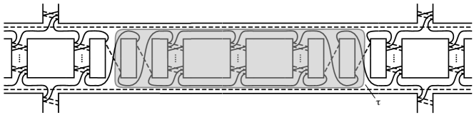
Figure 19. Constructing the flype box for $r=2$. The disk $\Delta$ is shaded and $\tau$ is its boundary.

Let $Y=B^{fl}\cup\mathcal{N}_{S^{3}}(K)$, where we choose the neighborhood $\mathcal{N}(K)$ so small so that $Y$ is a genus two handlebody. Note that $\mathcal{A}=\partial Y\cap H_{2}^{r}$ is a union of one or two annuli, depending on $K$. Furthermore set $\widehat{H}^{r}_{1}=H_{1}^{r}\cup Y,\,\,\widehat{H}^{r}_{2}=S^{3}\smallsetminus int(\widehat{H}^{r}_{1})$. Note also that $\mathcal{A}$ separates $H_{2}^{r}$ into two components one of which has closure $\widehat{H}^{r}_{2}$. We now show that the pared manifold $(\widehat{H}^{r}_{2},\mathcal{A})$ contains no essential annuli.

The core of $\mathcal{A}$ is a link $\widehat{K}^{r}$ on $\widehat{\Sigma}^{r}=\partial\widehat{H}^{r}_{1}=\partial\widehat{H}^{r}_{2}$. The link $\widehat{K}^{r}$ is carried by a new trellis $\widehat{\mathcal{T}}^{r}$ where $B^{fl}$ is replaced by a single vertical column (see Figure 20). The projection into $P$ of $K^{r}$ outside $B^{fl}$ is equal to the projection of $\widehat{K}^{r}$ outside this column.

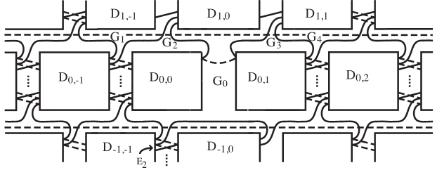
Figure 20. The new trellis $\widehat{\mathcal{T}}^{r}$, obtained by amalgamating the flype box and the columns it meets into one new column. The new column is here between $D_{0,0}$ and $D_{0,1}$.

We apply the same techniques as in the proof of Lemma 5.6. Note that there are four front $\mathcal{E}$ regions $G_{0},G_{1},G_{2},G_{3}$ whose configurations are somewhat different. The other front $\mathcal{E}$ regions stay the same. The back $\mathcal{E}$ regions stay the same but note that in the back of the new column there are no “small” regions connecting just $D^{-}_{0,0}$ and $D^{-}_{0,1}$, because there is only one arc in that column.

Note by inspection that all $\mathcal{E}$ regions are disks and that every region intersects each disk side in $\widehat{\mathcal{D}}$ in at most a single arc. In other words this recovers conditions (1-3) coming from Lemma 2.2 of [12], as used in Step (1) of Proposition 5.4. Therefore we can apply the same proof as in Step (1) to conclude that any annulus in $(\widehat{H}^{r}_{2},\mathcal{A})$, after suitable isotopy, is decomposed into a cycle of rectangles.

An inspection of the diagram yields the following new nontrivial rectangles. (There are also rectangles that have appeared in previous cases, and which are not listed below.)

Front rectangles

1. $(D^{+}_{-1,-1},D^{+}_{-1,0},G_{0},E_{i}),\,\,i\geq 3$. The regions $E_{i}$ are in the column between $D_{-1,-1}$ and $D_{-1,0}$, as indicated in Figure 20.

2. $(D^{+}_{0,1},D^{+}_{1,1},G_{0},G_{4})$

Back rectangles

We denote the “long” back regions in the layer of $D_{0,0}$ by $F$ and $F^{\prime}$, as in case (B3). We also enumerate the “small” back regions in the column between $D_{0,0}$ and $D_{0,-1}$ as $F^{-1}_{1},\ldots,F^{-1}_{q}$, and similarly the “small” back regions in the column between $D_{0,1}$ and $D_{0,2}$ as $F^{1}_{1},\ldots,F^{1}_{p}$. We then obtain:

1. $(D^{-}_{0,1},D^{-}_{0,i},F,F^{\prime}),\,\,i\neq 0$

2. $(D^{-}_{0,0},D^{-}_{0,i},F,F^{\prime}),\,\,i\neq 1$

The last two cases are of a type already discussed in (B4), but we mention them here because we must analyze their potential interaction with the new rectangles.

1. (a) $(D^{-}_{0,1},D^{-}_{0,2},F,F^{1}_{j}),\,\,2\leq j\leq p$ and
   (b) $(D^{-}_{0,1},D^{-}_{0,2},F^{\prime},F^{1}_{j}),\,\,1\leq j\leq p-1$.

2. (a) $(D^{-}_{0,0},D^{-}_{0,-1},F,F^{-1}_{j}),\,\,2\leq j\leq q$ and
   (b) $(D^{-}_{0,0},D^{-}_{0,-1},F^{\prime},F^{-1}_{j}),\,\,1\leq j\leq q-1$.

Note that the $\mathcal{E}$ region $G_{0}$ connects a large number of disks namely $D^{+}_{-1,-1},D^{+}_{-1,0},D^{+}_{1,0},D^{+}_{1,1},D^{+}_{0,0},D^{+}_{0,1}$ and $D^{+}_{0,2}$. However only a few of these participate in nontrivial rectangles as indicated in (C1) and (C2).

The rectangles in case (C1) are not adjacent to any rectangle along $D_{-1,0}$ using the same argument as in case (B1) in the proof of Lemma 5.9. The rectangle in (C2) is adjacent along $D_{0,1}$ to a rectangle in case (C5)(b), for $j=1$. That rectangle has no further adjacencies and hence cannot participate in a cycle.

In case (C3) the rectangles are adjacent on one side to a trivial rectangle. However on the other side they have no further adjacencies since there are no front rectangles meeting opposite horizontal edges of a disk (see the analysis of (B3) in Lemma 5.9). Case (C4) is handled similarly.

Case (C5) (a) The rectangles in this case have no adjacencies along $D_{0,1}$. The rectangles in case (b) have no adjacencies along $D_{0,2}$.

Case (C6) (a) The rectangles there have no adjacencies along $D_{0,-1}$. In case (b) the rectangles have no adjacencies along $D_{0,0}$.

The cases above together with the analysis in Lemma 5.9 show that non-trivial rectangles cannot participate in cycles. This proves that there are essential annuli in $(\widehat{H}^{r}_{2},\mathcal{A})$ and this completes the proof of the proposition.

∎

6. Finishing the proof

We can now assemble the previous results to produce a sequence of primitive stable discrete faithful representations with rank going to infinity which converges geometrically to a knot complement.

Proof of Theorem 1.1.

Let $K\subset S^{3}$ be a knot carried by a nice flypeable trellis $\mathcal{T}$ and satisfying the conditions of Theorem 4.1. The manifold $M_{\infty}=S^{3}-\operatorname{\mathcal{N}}(K)$ is hyperbolic by Proposition 5.2, so we have a discrete faithful representation $\eta:\pi_{1}(M_{\infty})\to PSL_{2}(\mathbb{C})$.

For each $r\in\mathbb{N}$, consider the decomposition of $M_{\infty}$ along $\Sigma^{r}\smallsetminus\operatorname{\mathcal{N}}(K^{r})$ into two handlebodies

$$V^{r}=H_{1}^{r}\smallsetminus\mathcal{N}(K^{r})$$

and

$$W^{r}=H_{2}^{r}\smallsetminus\mathcal{N}(K^{r}).$$

Let $i^{r}_{*}:\pi_{1}(V^{r})\to\pi_{1}(M_{\infty})$ be induced by the inclusion map. Recall that $\pi_{1}(V^{r})=F_{n_{r}}$, where $n_{r}=n_{0}+2r$.

(1)

We let $K_{\Sigma^{r}}(p/q)$ denote the $p/q$ Dehn filling of $K^{r}$ with respect to the framing of $\Sigma^{r}$ as in Subsection 4.2, where we have abbreviated $K_{\Sigma^{r}}=K^{r}_{\Sigma^{r}}$. For each $m\in\mathbb{Z}$, let $q_{m}:\pi_{1}(M_{\infty})\to\pi_{1}(K_{\Sigma^{r}}(1/m))$ be the quotient map induced by surgery.

By Thurston’s Dehn filling theorem, for large enough $|m|$ the manifolds $K_{\Sigma^{r}}(1/m)$ are hyperbolic, and there are discrete faithful representations $\eta_{m}:\pi_{1}(K_{\Sigma^{r}}(1/m))\to PSL_{2}(\mathbb{C})$ such that the representations $\eta_{m}\circ q_{m}$ converge to $\eta$. Moreover the quotient manifolds converge geometrically to $M_{\infty}$.

Because the surgered manifold $K_{\Sigma^{r}}(1/m)$ is obtained by an $m$-fold Dehn twist on $K^{r}$, the images of $V^{r}$ and $W^{r}$ determine a Heegaard splitting for this manifold, and in particular the map $q_{m}\circ i^{r}_{*}$ is surjective.

Letting $m\to\infty$, the representations $\rho^{r}_{m}=\eta_{m}\circ q_{m}\circ i^{r}_{*}$ converge to $\rho^{r}_{\infty}=\eta\circ i^{r}_{*}$.

The representation $\rho^{r}_{\infty}$ satisfies the hypotheses of Proposition 3.5: Hypothesis (1) (a cut point free Whitehead graph) follows from Lemma 5.1; hypothesis (2) (incompressibility of $\Sigma^{r}\smallsetminus K^{r}$) follows from Theorem 4.1; and hypothesis (3) (the pared manifold $(W^{r},\overline{\mathcal{N}}(K^{r})\cap\partial W^{r})$ is not an $I$ bundle) follows from Proposition 5.10. We conclude, by Proposition 3.5, that $\rho^{r}_{\infty}$ is primitive stable.

Since the primitive stable set $PS(F_{n_{r}})$ is open (see Minsky [15]), for each $r$ there exists $m_{r}$ such that $\rho^{r}_{m_{r}}$ is primitive stable as well. In particular the image of $\rho^{r}\equiv\rho^{r}_{m_{r}}$ is the whole group $\eta_{m_{r}}(\pi_{1}(K_{\Sigma^{r}}(1/m_{r}))$, and by choosing $m_{r}$ sufficiently large for each $r$, this sequence of groups converges geometrically to $\eta(\pi_{1}(M_{\infty}))$ as $r\to\infty$. This is the desired sequence of representations.

∎

References

- [1] I. Agol, Tameness of hyperbolic 3-manifolds, Preprint, 2004, arXiv:math.GT/0405568.
- [2] F. Bonahon, Bouts des variétés hyperboliques de dimension 3, Ann. of Math. 124 (1986), 71–158.
- [3] F. Bonahon, Geometric structures on 3-manifolds, Handbook of geometric topology, North-Holland, Amsterdam, 2002, pp. 93–164.
- [4] D. Calegari and D. Gabai, Shrinkwrapping and the taming of hyperbolic 3-manifolds, J. Amer. Math. Soc. 19 (2006), no. 2, 385–446 (electronic).
- [5] R. D. Canary, A covering theorem for hyperbolic 3-manifolds and its applications, Topology 35 (1996), 751–778.
- [6] J. Hempel, 3-manifolds, Annals of Math. Studies no. 86, Princeton University Press, 1976.
- [7] W. Jaco, Lectures on three-manifold topology, CBMS Regional Conference Series in Mathematics, vol. 43, American Mathematical Society, Providence, R.I., 1980.
- [8] W. H. Jaco and P. B. Shalen, Seifert fibered spaces in 3-manifolds, vol. 21, Memoirs of the Amer. Math. Soc., no. 220, A.M.S., 1979.
- [9] K. Johannson, Homotopy equivalences of 3-manifolds with boundary, Lecture Notes in Mathematics, vol. 761, Springer-Verlag, 1979.
- [10] R. S. Kulkarni and P. B. Shalen, On Ahlfors’ finiteness theorem, Adv. Math. 76 (1989), no. 2, 155–169.
- [11] A. Lubotzky, Dynamics of actions on group presentations and representations, Preprint, 2008.
- [12] M. Lustig and Y. Moriah, 3-manifolds with irreducible Heegaard splittings of high genus, Topology 39 (2000), no. 3, 589–618.
- [13] D. McCullough, Compact submanifolds of 3-manifolds with boundary, Quart. J. Math. Oxford 37 (1986), 299–306.
- [14] D. McCullough, A. Miller, and G. A. Swarup, Uniqueness of cores of noncompact -manifolds, J. London Math. Soc. (2) 32 (1985), no. 3, 548–556.
- [15] Y. Minsky, Note on dynamics of on -characters, Preprint, 2009, arXiv:0906.3491.
- [16] J. W. Morgan, On Thurston’s uniformization theorem for three-dimensional manifolds, The Smith Conjecture (H. Bass and J. Morgan, eds.), Academic Press, 1984, pp. 37–125.
- [17] Y. Moriah and J. Schultens, Irreducible Heegaard splittings of Seifert fibered spaces are either vertical or horizontal, Topology 37 (1998), no. 5, 1089–1112.
- [18] G. P. Scott, Compact submanifolds of 3-manifolds, J. London Math. Soc. 7 (1973), 246–250.
- [19] W. Thurston, The geometry and topology of 3-manifolds, Princeton University Lecture Notes, online at http://www.msri.org/publications/books/gt3m, 1982.
- [20] F. Waldhausen, On irreducible 3-manifolds which are sufficiently large, Ann. of Math. 87 (1968), 56–88.
- [21] J. H. C. Whitehead, On certain sets of elements in a free group, Proc. London Math. Soc. 41 (1936), 48–56.
- [22] by same author, On equivalent sets of elements in a free group, Annals of Math. 37 (1936), 782–800.