Optimal Power Allocation for Secrecy Fading Channels Under Spectrum-Sharing Constraints

Abstract

In the spectrum-sharing technology, a secondary user may utilize the primary user’s licensed band as long as its interference to the primary user is below a tolerable value. In this paper, we consider a scenario in which a secondary user is operating in the presence of both a primary user and an eavesdropper. Hence, the secondary user has both interference limitations and security considerations. In such a scenario, we study the secrecy capacity limits of opportunistic spectrum-sharing channels in fading environments and investigate the optimal power allocation for the secondary user under average and peak received power constraints at the primary user with global channel side information (CSI). Also, in the absence of the eavesdropper’s CSI, we study optimal power allocation under an average power constraint and propose a suboptimal on/off power control method.

Index Terms: Spectrum sharing, cognitive radio, physical-layer security, fading channel, power control.

I introduction

The proliferation of wireless systems and services has increased the need to efficiently use the scarce spectrum in wireless applications. This, together with the recently observed fact that the spectrum resources are not being utilized effectively, have spurred much interest in the study of cognitive radio networks. In cognitive radio networks, the secondary users may be allowed to transmit concurrently in the same frequency band with the primary users as long as the resulting interference power at the primary receivers is kept below the interference temperature limit [1]. A significant amount of work has been done to study the transmitter design under such interference constraints, e.g., in [2] and [3] for the fading channel, in [4] for the multiple-input multiple-output (MIMO) channel, in [5] for the relay channel.

On the other hand, the broadcast nature of wireless transmissions allows for the signals to be received by all users within the communication range, making wireless communications vulnerable to eavesdropping. The problem of secure transmission in the presence of an eavesdropper was first studied from an information-theoretic perspective in [6] where Wyner considered a wiretap channel model. Wyner showed that secure communication is possible without sharing a secret key if the eavesdropper’s channel is a degraded version of the main channel, and identified the rate-equivocation region and established the secrecy capacity of the degraded discrete memoryless wiretap channel. The secrecy capacity is defined as the maximum achievable rate from the transmitter to the legitimate receiver, which can be attained while keeping the eavesdropper completely ignorant of the transmitted messages. Later, Wyner’s result was extended to the Gaussian channel in [8] and recently to fading channels in [9] and [10]. In addition to the single antenna case, secrecy in multi-antenna models was addressed in [11] and [12]. Cooperative relaying under secrecy constraints was also recently studied in [13]–[15].

In this paper, we consider a scenario in which second users communicate in the presence of a primary user and an eavesdropper. Hence, secondary users need to both control the interference levels on the primary user and send the information securely. Hence, we combine the challenges seen in studies of cognitive radio networks and information-theoretic security. We note that, despite its practical relevance, security considerations in cognitive transmissions have received relatively little attention in research. Capacity of cognitive interference channel with secrecy is studied in [16]. Recently, [17] has studied secure communication over MISO cognitive radio channels. The secrecy capacity of the channel is characterized, and finding the capacity-achieving transmit covariance matrix under the joint transmit power and interference power constraints is formulated as a quasiconvex optimization problem.

Our contributions in this paper are as follows. We initially assume that the transmitter has global channel side information (CSI), i.e., perfectly knows the fading coefficients of all channels, and we study the secrecy capacity limits of opportunistic spectrum-sharing channels in fading environments and identify the optimal power allocation for the secondary user under average and peak received power constraints at the primary user. Subsequently, we consider the case in which the eavesdropper’s CSI is unavailable at the source. In this scenario, we study the optimal power allocation under average power constraints, and propose a simplified on/off power control method.

II Channel Model

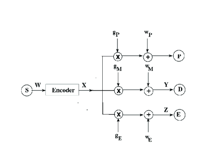
Figure 1: Channel Model

As depicted in Fig.1, we consider a cognitive radio channel model with a secondary user source $S$, a primary user $P$, a secondary user destination $D$, and an eavesdropper $E$. In this model, the source $S$ tries to transmit confidential messages to destination $D$ on the same band as the primary user’s while keeping the interference on the primary user below some predefined interference temperature limit and keeping the eavesdropper $E$ ignorant of the information. During any coherence interval $i$, the signal received by the destination and the eavesdropper are given, respectively, by

$$y(i) = g_{M}(i)x(i)+w_{M}(i),$$ (1)

$$z(i) = g_{E}(i)x(i)+w_{E}(i),$$ (2)

where $g_{M}(i),g_{E}(i)$ are the channel gains from the secondary source to the secondary receiver (main channel) and from the secondary source to the eavesdropper (eavesdropper channel), respectively, and $w_{M}(i),w_{E}(i)$ represent the i.i.d additive Gaussian noise with zero-mean and unit-variance at the destination and the eavesdropper, respectively. We denote the fading power gains of the main and eavesdropper channels by $h_{M}(i)=|g_{M}(i)|^{2}$ and $h_{E}(i)=|g_{E}(i)|^{2}$, respectively. Similarly, we denote the channel gain from the secondary source to the primary receiver by $g_{P}(i)$ and its fading power gain by $h_{P}(i)=|g_{P}(i)|^{2}$. We assume that both channels experience block fading, i.e., the channel gains remain constant during each coherence interval and change independently from one coherence interval to the next. The fading process is assumed to be ergodic with a bounded continuous distribution. Moreover, the fading coefficients of the destination and the eavesdropper in any coherence interval are assumed to be independent of each other.

Since transmissions pertaining to the secondary user should not harm the signal quality at the receiver of the primary user, we impose constraints on the received-power at the primary user $P$. Hence, denoting the average and peak received-power values by $Q_{avg}$ and $Q_{peak}$, respectively, we define the corresponding constraints as:

$$\mathbb{E}_{h_{M},h_{E},h_{P}}\{P(h_{M},h_{E},h_{P})h_{P}\}\leq Q_{avg}$$ (3)

and

$$P(h_{M},h_{E},h_{P})h_{P}\leq Q_{peak},~{}~{}~{}\forall h_{M},h_{E},h_{P}.$$ (4)

Note that $Q_{avg}$ can be seen as a long-term average received power constraint. Additionally, although we call $Q_{peak}$ as the peak received-power constraint, it is actually a peak constraint on the average instantaneous received power and can be regarded as a short-term constraint.

III Power Allocation under Average Received-Power Constraints

In a fading environment, following the the same line of development as in [10], it is straightforward but tedious to show that the channel capacity is achieved by optimally distributing the transmitted power over time such that the primary user received power constraint is met. By assuming that $h_{M}$, $h_{E}$, and $h_{P}$ are independent of each other and global CSI is available, the secrecy capacity under an average received power constraint is the solution to the following optimization problem,

$$\max_{P(h_{M},h_{E},h_{P})\geq 0}\int\int\int\Big{[}\log\left(1+h_{M}P(h_{M},h_{E},h_{P})\right)$$

$$\hskip 99.58464pt-\log\left(1+h_{E}P(h_{M},h_{E},h_{P})\right)\Big{]}^{+}$$

$$\hskip 93.89418pt\times f(h_{M})f(h_{E})f(h_{P}){\mathrm{d}}h_{M}{\mathrm{d}}h_{E}{\mathrm{d}}h_{P}$$

$$s.t~{}~{}~{}\int\int\int h_{P}P(h_{M},h_{E},h_{P})$$

$$~{}~{}~{}~{}~{}~{}~{}~{}~{}~{}~{}~{}~{}~{}\times f(h_{M})f(h_{E})f(h_{P}){\mathrm{d}}h_{M}{\mathrm{d}}h_{E}{\mathrm{d}}h_{P}\leq Q_{avg}$$ (5)

where $[x]^{+}=\max\{0,x\}$. To find the optimal power allocation $P(h_{M},h_{E},h_{P})$, we form the Lagrangian:

$$L(P,\lambda)=\int\int\int\Big{[}\log\left(1+h_{M}P(h_{M},h_{E},h_{P})\right)$$

$$-\log\left(1+h_{E}P(h_{M},h_{E},h_{P})\right)\Big{]}^{+}f(h_{M})f(h_{E})f(h_{P}){\mathrm{d}}h_{M}{\mathrm{d}}h_{E}{\mathrm{d}}h_{P}$$

$$-\lambda\Big{(}\int\int\int h_{P}P(h_{M},h_{E},h_{P})$$

$$~{}~{}~{}~{}\times f(h_{M})f(h_{E})f(h_{P}){\mathrm{d}}h_{M}{\mathrm{d}}h_{E}{\mathrm{d}}h_{P}-Q_{avg}\Big{)}.$$ (6)

By using the Lagrangian maximization approach, we get the following optimality condition:

$$\frac{\partial L(P,\lambda)}{\partial P(h_{M},h_{E},h_{P})}$$

$$=(\frac{h_{M}}{1+h_{M}P(h_{M},h_{E},h_{P})}-\frac{h_{E}}{1+h_{E}P(h_{M},h_{E},h_{P})}-\lambda h_{P})$$

$$\hskip 14.22636pt\times f(h_{M})f(h_{E})f(h_{P})~{}=~{}0.$$ (7)

Solving (III) with the constraint $P(h_{M},h_{E},h_{P})\geq 0$ yields the optimal power allocation policy at the transmitter as

$$P(h_{M},h_{E},h_{P})=\frac{1}{2}\Bigg{[}\sqrt{\left(\frac{1}{h_{E}}-\frac{1}{h_{M}}\right)^{2}+\frac{4}{\lambda h_{P}}\left(\frac{1}{h_{E}}-\frac{1}{h_{M}}\right)}$$

$$-\left(\frac{1}{h_{M}}+\frac{1}{h_{E}}\right)\Bigg{]}^{+},$$ (8)

where $\lambda$ is a constant that is introduced to satisfy the receive power constraint (5) at the primary user.

Remark 1

It is easy to see that when $h_{E}>h_{M}$, $P(h_{M},h_{E},h_{P})=0$, which is in accordance with our intuition. Transmitter only spends power for transmission when the main channel is better than the eavesdropper’s channel. With little calculation, we can also see that when $h_{P}>\frac{h_{M}-h_{E}}{\lambda}$, we have $P(h_{M},h_{E},h_{P})=0$. Thus, the power allocation can be rewritten as

$$P(h_{M},h_{E},h_{P})=\left\{\begin{array}[]{ll}\frac{1}{2}\Bigg{[}\sqrt{\left(\frac{1}{h_{E}}-\frac{1}{h_{M}}\right)^{2}+\frac{4}{\lambda h_{P}}\left(\frac{1}{h_{E}}-\frac{1}{h_{M}}\right)}\\ -\left(\frac{1}{h_{M}}+\frac{1}{h_{E}}\right)\Bigg{]}~{}~{}~{}~{}~{}~{}~{}\frac{h_{M}-h_{E}}{h_{P}}>\lambda\\ 0~{}~{}~{}~{}~{}~{}~{}~{}~{}~{}~{}~{}~{}~{}~{}~{}~{}~{}~{}~{}~{}~{}~{}~{}~{}~{}\frac{h_{M}-h_{E}}{h_{P}}\leq\lambda\end{array}\right..$$ (12)

Remark 2

From the expression of the optimal power allocation obtained in (III), we can easily see that more transmission power is used when either $h_{M}$ increases or $h_{P}$ decreases. Also the derivative of (III) with regard to $h_{E}$ is

$$-\frac{1}{2h_{E}^{2}}\Big{[}\frac{\frac{1}{h_{E}}-\frac{1}{h_{M}}+\frac{2}{\lambda h_{P}}}{\sqrt{\left(\frac{1}{h_{E}}-\frac{1}{h_{M}}\right)^{2}+\frac{4}{\lambda h_{P}}\left(\frac{1}{h_{E}}-\frac{1}{h_{M}}\right)}}-1\Big{]}.$$ (13)

We can see that the derivative is negative, so $P(h_{M},h_{E},h_{P})$ decreases when $h_{E}$ increases. These observations are also intuitively appealing. The secondary user takes advantage of the weak link between its transmitter and the primary receiver, and the stronger main channel. Also, a weaker eavesdropper’s channel is preferred for secure message transmission.

Remark 3

When there is no eavesdropper, the channel is the standard cognitive radio channel. By letting $h_{E}=0$ in (III) and solving the problem, we can obtain the optimal power allocation as $(\frac{1}{\lambda h_{P}}-\frac{1}{h_{M}})^{+}$, which has also been shown in [2] and [3].

Remark 4

When there is no primary user, the channel is the standard secrecy fading channel. By replacing $h_{P}$ with $1$ in (5) and correspondingly replacing $h_{P}$ with $1$ in (III), we get the optimal power allocation for the fading secrecy channel given in [10].

IV Power Allocation under both Average and Peak Received-Power Constraints

The average received power constraint is reasonable when the primary user’s QoS is determined by the average long-term interference. However, we note that in many cases, the primary user’s QoS is also limited by the instantaneous interference at the primary receiver. With this motivation, we in this section study the power allocation under both average and peak received power constraints.

We first introduce a real-valued function $\beta$ which is defined as

$$\beta^{2}\triangleq\frac{Q_{peak}}{h_{P}}-P(h_{M},h_{E},h_{P}).$$ (14)

To satisfy the peak power constraint, the right-hand side of (14) must be nonnegative over all the possible values of the channel gain. Using (14), we form an equivalent problem of (5), which contains an equality constraint for the peak power.

$$\max_{P(h_{M},h_{E},h_{P})\geq 0,\beta}\int\int\int\Big{[}\log\left(1+h_{M}P(h_{M},h_{E},h_{P})\right)$$

$$\hskip 99.58464pt-\log\left(1+h_{E}P(h_{M},h_{E},h_{P})\right)\Big{]}^{+}$$

$$\hskip 93.89418pt\times f(h_{M})f(h_{E})f(h_{P}){\mathrm{d}}h_{M}{\mathrm{d}}h_{E}{\mathrm{d}}h_{P}$$ (15)

$$s.t~{}~{}~{}\int\int\int h_{P}P(h_{M},h_{E},h_{P})$$

$$~{}~{}~{}~{}~{}~{}~{}~{}~{}~{}~{}~{}~{}~{}\times f(h_{M})f(h_{E})f(h_{P}){\mathrm{d}}h_{M}{\mathrm{d}}h_{E}{\mathrm{d}}h_{P}\leq Q_{avg}\$$ (16)

$$\text{and}~{}~{}~{}~{}~{}~{}~{}~{}~{}~{}~{}\beta^{2}+P(h_{M},h_{E},h_{P})=\frac{Q_{peak}}{h_{P}}.$$ (17)

Now, the Lagrangian becomes

$$L(P,\lambda)=\int\int\int\Big{[}\log\left(1+h_{M}P(h_{M},h_{E},h_{P})\right)$$

$$-\log\left(1+h_{E}P(h_{M},h_{E},h_{P})\right)\Big{]}^{+}f(h_{M})f(h_{E})f(h_{P}){\mathrm{d}}h_{M}{\mathrm{d}}h_{E}{\mathrm{d}}h_{P}$$

$$-\lambda\Big{(}\int\int\int h_{P}P(h_{M},h_{E},h_{P})$$

$$~{}~{}~{}~{}\times f(h_{M})f(h_{E})f(h_{P}){\mathrm{d}}h_{M}{\mathrm{d}}h_{E}{\mathrm{d}}h_{P}-Q_{avg}\Big{)}$$

$$-\lambda_{0}\Big{(}\beta^{2}+P(h_{M},h_{E},h_{P})-\frac{Q_{peak}}{h_{P}}\Big{)}.$$ (18)

Setting each of the partial derivatives of the Lagrangian with respect to $P$ and $\beta$ to zero, we obtain, respectively, the necessary conditions for the optimal solution to problem (17) as

$$\frac{h_{M}}{1+h_{M}P(h_{M},h_{E},h_{P})}- \frac{h_{E}}{1+h_{E}P(h_{M},h_{E},h_{P})}-\lambda h_{P}-\lambda_{0}=0$$ (19)

$$2\beta\lambda_{0}=0.$$ (20)

Note that (20) implies either $\beta=0$ or $\lambda_{0}=0$. $\beta=0$ means that the peak power constraint is active and hence, the optimal transmission power in this case is given by (21)

$$P(h_{M},h_{E},h_{P})=\frac{Q_{peak}}{h_{P}}.$$ (21)

On the other hand, $\lambda_{0}=0$ in (20) means that the peak transmission power constraint is inactive and it can be ignored. Solving (19) with $\lambda_{0}=0$, we get the expression for the optimal transmitter power as

$$\frac{1}{2}\Bigg{[}\sqrt{\left(\frac{1}{h_{E}}-\frac{1}{h_{M}}\right)^{2}+\frac{4}{\lambda h_{P}}\left(\frac{1}{h_{E}}-\frac{1}{h_{M}}\right)}-\left(\frac{1}{h_{M}}+\frac{1}{h_{E}}\right)\Bigg{]}^{+},$$

which is the same expression as in (III) obtained when there is only an average received power constraint. Combining the two cases, the optimal power allocation under both average and peak power constraints becomes

$$\hskip 28.45274ptP(h_{M},h_{E},h_{P})=\min\Bigg{(}\frac{Q_{peak}}{h_{P}},$$

$$\frac{1}{2}\Bigg{[}\sqrt{\left(\frac{1}{h_{E}}-\frac{1}{h_{M}}\right)^{2}+\frac{4}{\lambda h_{P}}\left(\frac{1}{h_{E}}-\frac{1}{h_{M}}\right)}-\left(\frac{1}{h_{M}}+\frac{1}{h_{E}}\right)\Bigg{]}^{+}\Bigg{)}$$ (22)

where $\lambda$ is a constant with which the average power constraint is satisfied. We should note that $\lambda$ here is generally not the same as $\lambda$ in the optimal power allocation in (III).

Remark 5

We can see from (IV) with little computation that when the condition

$$\frac{1}{\frac{h_{E}}{h_{P}}+1/Q_{peak}}-\frac{1}{\frac{h_{M}}{h_{P}}+1/Q_{peak}}>\lambda Q_{peak}^{2}$$ (23)

is satisfied, we have $P(h_{M},h_{E},h_{P})=\frac{Q_{peak}}{h_{P}}$

V Power Allocation without Eavesdropper’s CSI

Since eavesdropping is a passive operation (i.e., does not involve any transmission), the source may not be able to get the CSI of the eavesdropper’s channel in certain circumstances. With this motivation, we in this section study the optimal power allocation when the source knows only $h_{M}$ and $h_{P}$. To simplify the analysis, we consider only average receive power constraints here.

V-A Optimal Power Allocation

Based on the results of [10], the secrecy capacity in this case is the solution of the following optimization problem:

$$\max_{P(h_{M},h_{P})\geq 0}\int\int\int\Big{[}\log\left(1+h_{M}P(h_{M},h_{P})\right)$$

$$\hskip 99.58464pt-\log\left(1+h_{E}P(h_{M},h_{P})\right)\Big{]}^{+}$$

$$\hskip 93.89418pt\times f(h_{M})f(h_{E})f(h_{P}){\mathrm{d}}h_{M}{\mathrm{d}}h_{E}{\mathrm{d}}h_{P}$$

$$s.t~{}~{}~{}\int\int\int h_{P}P(h_{M},h_{P})$$

$$~{}~{}~{}~{}~{}~{}~{}~{}~{}~{}~{}~{}~{}~{}\times f(h_{M})f(h_{E})f(h_{P}){\mathrm{d}}h_{M}{\mathrm{d}}h_{E}{\mathrm{d}}h_{P}\leq Q_{avg}.$$ (24)

Similarly, using the Lagrangian approach, we get the optimal condition as

$$\frac{h_{M}\Pr\left(h_{E}\leq h_{M}\right)}{1+h_{M}P(h_{M},h_{P})}$$

$$-\int_{0}^{h_{M}} \left(\frac{h_{E}}{1+h_{E}P(h_{M},h_{P})}\right)f(h_{E}){\mathrm{d}}h_{E}-\lambda h_{P}~{}=~{}0,$$ (25)

where $\lambda$ is a constant that satisfies the power constraints in (24) with equality. By solving (V-A), we can get the optimal transmit power allocation $P(h_{M},h_{P})$. If the obtained value turns out to be negative, then the optimal value of $P(h_{M},h_{P})$ is equal to 0. The exact solution to this optimization problem depends on the fading distributions.

If Rayleigh fading scenario is considered with ${\mathbb{E}}\{h_{M}\}=\overline{\gamma}_{M}$, ${\mathbb{E}}\{h_{E}\}=\overline{\gamma}_{E}$ and ${\mathbb{E}}\{h_{P}\}=\overline{\gamma}_{P}$ , then the optimal power allocation is the solution of the following equation:

$$\left(1-e^{-(h_{M}/\overline{\gamma}_{E})}\right)\left(\frac{h_{M}}{1+h_{M}P(h_{M},h_{P})}\right)\lambda h_{P}$$

$$-\frac{\left(1-e^{-(h_{M}/\overline{\gamma}_{E})}\right)}{P(h_{M},h_{P})}+\frac{\exp\left(\frac{1}{\overline{\gamma}_{E}P(h_{M},h_{P})}\right)}{\overline{\gamma}_{E}(P(h_{M},h_{P}))^{2}}\Bigg{[}\textrm{Ei}\left(\frac{1}{\overline{\gamma}_{E}P(h_{M},h_{P})}\right)$$

$$-\textrm{Ei}\left(\frac{h_{M}}{\overline{\gamma}_{E}}+\frac{1}{\overline{\gamma}_{E}P(h_{M},h_{P})}\right)\Bigg{]}~{}=~{}0$$ (26)

where $\textrm{Ei}(x)~{}=~{}\int_{x}^{\infty}\frac{e^{-t}}{t}~{}{\mathrm{d}}t$ is the exponential integral function. Again, if there is no positive solution to (V-A), the optimal $P(h_{M},h_{P})=0$.

V-B On/Off power control

As seen above, the computation of the optimal power allocation is in general complicated. In this section, we use a simplified suboptimal on/off power control method [10]. That is, the source sends information only when the channel gain $h_{M}$ exceeds a pre-determined constant threshold $\tau>0$. Moreover, when $h_{M}>\tau$, the transmitter always uses the same power level $P$ . It is easy to compute that the constant power level used for transmission should be

$$P=\frac{Q_{avg}}{\overline{\gamma}_{P}\Pr(h_{M}>\tau)}.$$ (27)

For the Rayleigh fading scenario for which $f(h_{M})=\frac{1}{\overline{\gamma}_{M}}e^{-(h_{M}/\overline{\gamma}_{M})}$, we get

$$P=\frac{Q_{avg}}{\overline{\gamma}_{P}}e^{(\tau/\overline{\gamma}_{M})}.$$ (28)

Then, the secrecy rate can be computed as

$$R_{s}=\int_{0}^{\infty}\int_{\tau}^{\infty}\left[\log\left(1+h_{M}P\right)-\log\left(1+h_{E}P\right)\right]^{+}$$

$$\hskip 56.9055pt\times f(h_{M})f(h_{E}){\mathrm{d}}h_{M}{\mathrm{d}}h_{E}$$

$$=e^{-(\tau/\overline{\gamma}_{M})}\log\left(1+\tau\frac{Q_{avg}}{\overline{\gamma}_{P}}e^{(\tau/\overline{\gamma}_{M})}\right)+\exp\left(\frac{1}{\overline{\gamma}_{M}\frac{Q_{avg}}{\overline{\gamma}_{P}}e^{(\tau/\overline{\gamma}_{M})}}\right)$$

$$\textrm{Ei}\left(\frac{\tau}{\overline{\gamma}_{M}}+\frac{1}{\overline{\gamma}_{M}\frac{Q_{avg}}{\overline{\gamma}_{P}}e^{(\tau/\overline{\gamma}_{M})}}\right)+\exp\left(\frac{1}{\overline{\gamma}_{E}\frac{Q_{avg}}{\overline{\gamma}_{P}}e^{(\tau/\overline{\gamma}_{M})}}-\frac{\tau}{\overline{\gamma}_{M}}\right)$$

$$\left[\textrm{Ei}\left(\frac{\tau}{\overline{\gamma}_{E}}+\frac{1}{\overline{\gamma}_{E}\frac{Q_{avg}}{\overline{\gamma}_{P}}e^{(\tau/\overline{\gamma}_{M})}}\right)-\textrm{Ei}\left(\frac{1}{\overline{\gamma}_{E}\frac{Q_{avg}}{\overline{\gamma}_{P}}e^{(\tau/\overline{\gamma}_{M})}}\right)\right]$$

$$-\exp\left(\frac{\left[\frac{1}{\overline{\gamma}_{M}}+\frac{1}{\overline{\gamma}_{E}}\right]}{\frac{Q_{avg}}{\overline{\gamma}_{P}}e^{(\tau/\overline{\gamma}_{M})}}\right)\textrm{Ei}\left(\left[\frac{1}{\overline{\gamma}_{M}}+\frac{1}{\overline{\gamma}_{E}}\right]\left[\tau+\frac{1}{\frac{Q_{avg}}{\overline{\gamma}_{P}}e^{(\tau/\overline{\gamma}_{M})}}\right]\right).$$ (29)

Note that the secrecy rate depends on the threshold $\tau$. Hence, we can get the maximum achievable secrecy rate under the on/off power control policy by optimizing the threshold $\tau$.

VI Numerical Results

In this section, we numerically illustrate the secrecy rate studied in this paper. In all simulations, we assume that the fading is Rayleigh distributed.

We first consider the case in which the global CSI is available. In Fig. 2, we plot the secrecy rate versus $Q_{avg}$ for different values of the peak received power constraint $Q_{peak}$. We can see from the figure that, as expected, the larger the $Q_{peak}$, the closer the rate is to the case of no peak power constraint. We also observe that the constraint on the peak received power does not have much impact on the secrecy rate for low values of $Q_{avg}$. On the other hand, as the value of the average received power limit approaches the peak received power constraint, the rate plots become flat and the performance gets essentially limited by the peak received-power constraint.

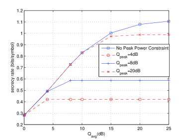
Figure 2: secrecy rate vs. $Q_{avg}$ for different peak power constraint with global CSI available, $\overline{\gamma}_{M}=\overline{\gamma}_{E}=1,\overline{\gamma}_{P}=2$.

In Fig. 3, we plot the ergodic secrecy rate as a function of $Q_{avg}$ while keeping the ratio $\frac{Q_{peak}}{Q_{avg}}$ fixed. We should point out that eavesdropper’s channel is stronger than the main channel on average (i.e., $\overline{\gamma}_{M}=1<\overline{\gamma}_{E}=2$) in this figure. Note that positive secrecy rate can not achieved without fading in such a case. In the figure, we again see that the higher the ratio $\frac{Q_{peak}}{Q_{avg}}$, the closer the curve is to the no peak power constraint case. Also, since the peak power constraint becomes more relaxed with increasing $Q_{avg}$, we do not see the flattening of the rate curve in contrast to what is observed in Fig. 2.

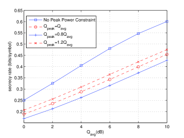
Figure 3: secrecy rate vs. $Q_{avg}$ for different peak power constraint with global CSI available, $\overline{\gamma}_{M}=1,\overline{\gamma}_{E}=2,\overline{\gamma}_{P}=2$.

Next, we consider the case in which the eavesdropper’s CSI is not available. In Fig.4, we plot the ergodic secrecy rate vs. $Q_{avg}$ curves achieved with optimal power allocation and with the on/off power control method. The fading variances $\bar{\lambda}$ are the same as in Fig. 3. By comparing the secrecy rates in Fig. 4 with the secrecy rate in Fig. 3 obtained in the absence of peak constraints, we observe that not having the eavesdropper’s channel information result in a certain loss in the secrecy rate. We also see that the performance of the on/off power control scheme is very close to the optimal secrecy capacity (when only the main channel and primary channel CSI is available) for a wide range of SNRs, and approach the optimal rate when SNR is high. Note that the optimality of the on/off power control scheme at high SNRs has been proved in [10] for the secrecy fading channel. Thus, the on/off power control method has great utility in practical systems due to its advantage of simple implementation.

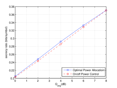
Figure 4: secrecy rate vs. $Q_{avg}$ without eavesdropper’s CSI, $\overline{\gamma}_{M}=1,\overline{\gamma}_{E}=2,\overline{\gamma}_{P}=2$.

VII Conclusion

In this paper, we have considered a spectrum-sharing system subject to security considerations and studied the optimal power allocation strategies for the secrecy fading channel under average and peak received power constraints at the primary user. In particular, we have considered two scenarios regarding the availability of the CSI. When global CSI is available, we have obtained analytical expressions for the optimal power allocation under average and peak received power constraints. When only main channel’s and primary channel’s CSI is available, we have characterized the optimal power allocation as the solution to a certain equation. We have also derived the analytical secrecy rate expression for the simplified on/off power control scheme in this scenario. Numerical results corroborating our theoretical analysis have also been provided. Specially, it is shown that the constraint on the peak received power does not have much impact on the secrecy rate for low values of $Q_{avg}$ as long as the average power constraints remain active, and that the performance of the suboptimal on/off power control scheme approaches the optimal performance when the eavesdropper’s CSI is not available.

References

- [1] S. Haykin, “Cognitive radio: brain-empowered wireless communicatioins,” IEEE J. Sel. Areas Commun, vol.23, no.2, pp.201-220, Feb 2005.
- [2] A. Ghasemi and E. S. Sousa, “Fundamental Limits of spectrum-sharing in fading environments,” IEEE Trans. Wireless. Commun, vol.6, no.2, pp.649-658, Feb 2007.
- [3] L. Musavian,and S. Aissa, “Capacity and power allocation for spectrum-sharing communications in fading channels ,” IEEE Trans. Wireless. Commun, vol.8, no.1, pp.148-156, Jan. 2009.
- [4] R. Zhang, and Y-C. Liang, “Exploiting multi-antenna for opportunistic spectrum sharing in cognitive radio networks,” IEEE J. Sel. Topics Signal Process., vol. 2, pp. 88 - 102, Feb. 2008.
- [5] J. Mietzner, L. Lampe, and R. Schober, “Distributed Transmit Power Allocation for Multihop Cognitive-Radio Systems,” IEEE Trans. Wireless. Commun,vol. 8, no. 10, pp. 5187-5201, Oct. 2009.
- [6] A. Wyner, “The wire-tap channel,” Bell. Syst Tech. J, vol.54, no.8, pp.1355-1387, Jan 1975.
- [7] I. Csiszar and J. Korner, “Broadcast channels with confidential messages,” IEEE Trans. Inform. Theory, vol.IT-24, no.3, pp.339-348, May 1978.
- [8] S. K. Leung-Yan-Cheong and M. E. Hellman, “The Gaussian wire-tap channel,” IEEE Trans. Inform. Theory, vol.IT-24, no.4, pp.451-456, July 1978.
- [9] Y. Liang, H. V. Poor, and S. Shamai (Shitz), “Secure communication over fading channels,” IEEE Trans. Inform. Theory, vol. 54, pp. 2470 - 2492, June 2008.
- [10] P. K. Gopala, L. Lai, and H. E. Gamal, “On the secrecy capacity of fading channels” IEEE Trans. Inform. Theory, vol.54, no.10, pp.4687-4698, Oct 2008.
- [11] S. Shafiee and S. Ulukus, “Achievable rates in Gaussian MISO channels with secrecy constraint,” IEEE Intl Symp. on Inform. Theory, Nice, France, June 2007.
- [12] A. Khisti, “ Algorithms and architectures for multiuser, multiterminal, and multilayer information-theoretic security ” Doctoral Thesis, MIT 2008.
- [13] L. Dong, Z. Han, A. Petropulu and H. V. Poor, “Secure wireless communications via cooperation,” Proc. 46th Annual Allerton Conf. Commun., Control, and Computing, Monticello, IL, Sept. 2008.
- [14] J. Zhang and M. C. Gursoy, “Collaborative relay beamforming for secrecy,” Proc. of the IEEE International Conference on Communication (ICC), Cape Town, South Africa, May 2010.
- [15] J. Zhang and M.C. Gursoy, “Relay Beamforming Strategies for Physical-Layer Security,” Proc. of the 44th Annual Conference on Information Sciences and Systems, Princeton, March 2010
- [16] Y. Liang, A. S-Baruch, H. V. Poor, and S. Shamai (Shitz), “Capacity of Cognitive Interference Channels With and Without Secrecy,” IEEE Trans. Inform. Theory, vol. 55 no. 2, pp. 604 - 619, Feb 2009.
- [17] Y. Pei, Y-C. Liang, L. Zhang, K. C. Teh, and K. H. Li, “Secure Coommunication Over MISO Cognitive Radio Channel,” IEEE Trans. Wireless. Commun, vol.9, no.4, pp.1494-1502, April. 2010.