Holographic field theory models of dark energy in interaction with dark matter

Abstract

We discuss two lagrangian interacting dark energy models in the context of the holographic principle. The potentials of the interacting fields are constructed. The models are compared with CMB distance information, baryonic acoustic oscilations, lookback time and the Constitution supernovae sample. For both models the results are consistent with a non vanishing interaction in the dark sector of the universe - with more than three standard deviations of confidence for one of them. Moreover, in both cases, the sign of coupling is consistent with dark energy decaying into dark matter, alleviating the coincidence problem.

I Introduction

In the last years, there have been several papers where an interaction in the dark sector of the universe is considered 1 - sandro3 . A motivation to considering the interaction is that dark energy and dark matter will evolve coupled to each other, alleviating the coincidence problem 1 . A further motivation is that, assuming dark energy to be a field, it would be more natural that it couples with the remaining fields of the theory, in particular with dark matter, as it is quite a general fact that different fields generally couple. In other words, it is reasonable to assume that there is no symmetry preventing such a coupling between dark energy and dark matter fields. Using a combination of several observational datasets, as supernovae data, CMB shift parameter, BAO, etc., it has been found that the coupling constant is small but non vanishing within at least $1\sigma$ confidence level 1 - sandro2 . In two recent works, the effect of an interaction between dark energy and dark matter on the dynamics of galaxy clusters was investigated through the Layser-Irvine equation, the relativistic equivalent of virial theorem peebles . Using galaxy cluster data, it has been shown that a non vanishing interaction is preferred to describe the data within several standard deviations virial . However, in most of these papers, the interaction term in the equation of motion is derived from phenomenological arguments. It is interesting to obtain the interaction term from a field theory. Some works have already taken a step in such a direction sandro2 , sandro3 , bean . On the other hand, scalar fields have been largely used as candidates to dark energy. They naturally arise in particle physics and string theory. Good reviews on this subject can be found in copeland . A motivation to use scalar fields as candidates to dark energy is that their pressure can be negative, making possible to reproduce the recent period of accelerated expansion of the universe. For example, for canonical scalar field, the equation of state parameter varies between $1$ and $-1$. Dark energy modeled as a canonical scalar field is called quintessence and was investigated, for example, in bean , canonico . For tachyon scalar field, the equation of state is always negative. The tachyon field has been studied in recent years in the context of string theory, as a low energy effective theory of D-branes and open strings sen . Tachyon field as dark energy was studied, for example, in sandro2 , taquions , taqholo . The first question about scalar fields concerns the choice of the potential. Common choices are the power law and the exponential potentials. However, these choices are in fact arbitrary. In principle, any other form for the potential which leads to recent accelerated expansion would be acceptable.

On the other hand, it is possible that a complete understanding of the nature of dark energy will only be possible within a quantum gravity theory context. Although results for quantum gravity are still missing, or at least premature, it is possible to introduce, phenomenologically, some of its principles in a model of dark energy. Recently combinations of quintessence, quintom and tachyon models with holographic dark energy had been proposed - in escalarholo , quintomholo and taqholo , respectively. Specifically, by imposing that the energy density of the scalar field must match the holographic dark energy density, namely $\rho_{\Lambda}=3c^{2}M_{Pl}^{2}L^{-2}$, where $c$ is a numerical constant and $L$ is the infrared cutoff, it was demonstrated that the equation of motion of fields for the non-interacting case reproduces the equation of motion for holographic dark energy. In fact, to impose that the energy density of scalar field must match the holographic dark energy density corresponds to specify its potential. This can be seen as a physical criterion to choose the potential. Here, we generalize this idea for two kinds of interacting scalar fields.

II The models

We consider the general action

$$S=\int d^{4}x\sqrt{-g}\left\{\frac{M_{Pl}^{2}}{2}R+\mathcal{L}_{\varphi}\left(x\right)+\frac{i}{2}[\bar{\Psi}\gamma^{\mu}\nabla_{\mu}\Psi-\bar{\Psi}\overleftarrow{\nabla}_{\mu}\gamma^{\mu}\Psi]-(M-\beta\varphi)\bar{\Psi}\Psi+\sum\limits_{j}\mathcal{L}_{j}\left(x\right)\right\}$$ (1)

where $M_{Pl}\equiv\left(8\pi G\right)^{-1/2}$ is the reduced Planck mass, $R$ is the curvature scalar, $\mathcal{L}_{\varphi}\left(x\right)$ is, unless of the coupling term, the lagrangian density for the scalar field, which we will identify with dark energy, $\Psi$ is a massive fermionic field, which we will identify with dark matter, $\beta$ is the dimensionless coupling constant and $\sum\limits_{j}\mathcal{L}_{j}\left(x\right)$ contains the lagrangian densities for the ramaining fields. Notice that, in this work, we will only consider an interaction of dark energy with dark matter. If there was a coupling between the scalar field and baryonic matter, the corresponding coupling constant $\beta_{b}$ should satisfy the solar system constraint solarsystem

$$\beta_{b}\lesssim 10^{-2}\text{ .}$$ (2)

We assume $\beta_{b}\equiv 0$, which trivially satisfy the constraint (2).

We consider two kinds of scalar fields: the canonical scalar field, or quintessence field, for which

$$\mathcal{L}_{\varphi}\left(x\right)=\frac{1}{2}\partial_{\mu}\varphi\partial^{\mu}\varphi-V(\varphi)\text{ ,}$$ (3)

and the tachyon scalar field, for which

$$\mathcal{L}_{\varphi}\left(x\right)=-V(\varphi)\sqrt{1-\alpha\partial^{\mu}\varphi\partial_{\mu}\varphi}\text{ ,}$$ (4)

where $\alpha$ is a constant with dimension $MeV^{-4}$. Notice that in both cases, we assume a Yukawa coupling with the dark matter field $\Psi$.

II.1 Quintessence field

For the quintessence field, $\mathcal{L}_{\varphi}\left(x\right)$ in the action (1) is given by (3). From a variational principle, we obtain

$$i\gamma^{\mu}\nabla_{\mu}\Psi-M^{\ast}\Psi=0\text{ ,}$$ (5)

$$i(\nabla_{\mu}\bar{\Psi})\gamma^{\mu}+M^{\ast}\bar{\Psi}=0\text{ ,}$$ (6)

where $M^{\ast}\equiv M-\beta\varphi$, and

$$\nabla_{\mu}\partial^{\mu}\varphi+\frac{dV(\varphi)}{d\varphi}=\beta\bar{\Psi}\Psi\text{ .}$$ (7)

Eqs. (5) and (6) are, respectively, the covariant Dirac equation and its adjoint, in the case of a non vanishing interaction between the Dirac field and the scalar field $\varphi$. For homogeneous fields and adopting the Friedmann-Robertson-Walker metric, $g_{\mu\nu}$=diag$\left(1,-a^{2}\left(t\right),-a^{2}\left(t\right),-a^{2}\left(t\right)\right)$, where $a^{2}\left(t\right)$ is the scale factor, eqs. (5) and (6) lead to

$$\frac{d(a^{3}\bar{\Psi}\Psi)}{dt}=0$$

which is equivalent to

$$\bar{\Psi}\Psi=\bar{\Psi}_{0}\Psi_{0}\left(\frac{a_{0}}{a}\right)^{3}$$ (8)

and (7) reduces to

$$\ddot{\varphi}+3H\dot{\varphi}+\frac{dV(\varphi)}{d\varphi}=\beta\bar{\Psi}\Psi\text{ ,}$$ (9)

where $H\equiv\frac{\dot{a}}{a}$ is the Hubble parameter.

From the energy-momentum tensor, we get

$$\rho_{\varphi} =\frac{1}{2}\dot{\varphi}^{2}+V(\varphi)\text{ ,}$$ (10)

$$P_{\varphi} =\frac{1}{2}\dot{\varphi}^{2}-V(\varphi)\text{ ,}$$ (11)

$$\rho_{\Psi} =M^{\ast}\bar{\Psi}\Psi\text{ ,}$$ (12)

$$P_{\Psi} =0\text{ .}$$

From (10) and (11) we have $\omega_{\varphi}\equiv\frac{P_{\varphi}}{\rho_{\varphi}}=\frac{\frac{1}{2}\dot{\varphi}^{2}-V(\varphi)}{\frac{1}{2}\dot{\varphi}^{2}+V(\varphi)}$. Deriving (10) and (12) with respect to time and using (8) and (9), we obtain

$$\dot{\rho}_{\varphi}+3H\rho_{\varphi}(\omega_{\varphi}+1)=\beta\dot{\varphi}\bar{\Psi}_{0}\Psi_{0}\left(\frac{a_{0}}{a}\right)^{3}$$ (13)

and

$$\dot{\rho}_{\Psi}+3H\rho_{\Psi}=-\beta\dot{\varphi}\bar{\Psi}_{0}\Psi_{0}\left(\frac{a_{0}}{a}\right)^{3}\text{ ,}$$ (14)

where the dot represents derivative with respect to time.

For baryonic matter and radiation, we have respectively

$$\dot{\rho}_{b}+3H\rho_{b}=0$$ (15)

and

$$\dot{\rho}_{r}+3H\rho_{r}(\omega_{r}+1)=0\text{ ,}$$ (16)

where $\omega_{r}=\frac{1}{3}$. Eqs. (15) and (16) implies that $\rho_{b}=\frac{\rho_{b0}}{a^{3}}$ and $\rho_{r}=\frac{\rho_{r0}}{a^{4}}$, respectively. The subscript $0$ denotes the quantities today. We are considering the radiation as composed by photons and massless neutrinos, so that $\rho_{r0}=\left(1+0.2271N_{eff}\right)\rho_{\gamma 0}$, where $N_{eff}=3.04$ is the effective number of relativistic degrees of freedom and $\rho_{\gamma 0}$ is the energy density of photons, given by $\rho_{\gamma 0}=\frac{\pi^{2}}{15}T_{CMB}$, being $T_{CMB}=2.725K$ the CMB temperature today. The Friedmann equation for a flat universe reads

$$H^{2}=\frac{1}{3M_{Pl}^{2}}\left[M^{\ast}\bar{\Psi}_{0}\Psi_{0}\left(\frac{a_{0}}{a}\right)^{3}+\frac{1}{2}\dot{\varphi}^{2}+V(\varphi)+\frac{\rho_{b0}}{a^{3}}+\frac{\rho_{r0}}{a^{4}}\right]\text{ .}$$ (17)

In order to determine the dynamics of the interacting quintessence field, it is necessary to specify the potential $V(\varphi)$. Instead of choosing an explicit form for $V(\varphi)$, we will specify it implicitly, by imposing that the energy density of the quintessence field, given by (10), must match the holographic dark energy density, $\rho_{\Lambda}=3c^{2}M_{Pl}^{2}L^{-2}$, where $c$ is a numerical constant and $L$ is the infrared cutoff. The evolution of the interacting quintessence field with redshift will be given by the equation of evolution for the holographic dark energy density, with a certain expression for the equation of state parameter $\omega_{\varphi}$. In fact, we will see that imposing the energy density of the quintessence field to match the holographic dark energy density leads to an expression for the potential.

In Li it has been argued that, in order that holographic dark energy drives the recent period of accelerated expansion, the IR cutoff $L$ must be the event horizon $R_{h}=a\left(t\right)\int_{t}^{\infty}\frac{dt^{\prime}}{a\left(t^{\prime}\right)}$. Substituting $R_{h}$ in the expression of the holographic dark energy, we get $R_{h}=\frac{c}{H\sqrt{\Omega_{\varphi}}}$, therefore,

$$\int_{t}^{\infty}\frac{dt^{\prime}}{a\left(t^{\prime}\right)}=\frac{c}{a\left(t\right)H\sqrt{\Omega_{\varphi}}}\text{ .}$$

Differentiating both sides with respect to time, using the Friedmann equation (17) together with conservation equations (13) and (14), we obtain

$$\frac{d\Omega_{\varphi}}{dz}=-\frac{\Omega_{\varphi}}{1+z}\left(2\frac{\sqrt{\Omega_{\varphi}}}{c}+3\Omega_{\varphi}\omega_{\varphi}+\Omega_{r}+1\right)\text{ .}$$ (18)

Equation (18) is just the equation of evolution for the holographic dark energy Li . Using the Friedmann equation (17), the conservation equations (15) and (16) can be written as

$$\frac{d\Omega_{b}}{dz}=-\frac{\Omega_{b}}{1+z}\left(3\Omega_{\varphi}\omega_{\varphi}+\Omega_{r}\right)$$ (19)

and

$$\frac{d\Omega_{r}}{dz}=-\frac{\Omega_{r}}{1+z}\left(3\Omega_{\varphi}\omega_{\varphi}+\Omega_{r}-1\right)\text{ .}$$ (20)

We define $r\equiv\frac{\rho_{\Psi}}{\rho_{\varphi}}$. Deriving $r$ with respect to time, using (13), (14), (10) and (11) we obtain

$$\dot{r}=3Hr\omega_{\varphi}-sign\left[\dot{\varphi}\right]\frac{\beta\left(1+r\right)}{\sqrt{3}M_{Pl}H}\sqrt{\frac{1+\omega_{\varphi}}{\Omega_{\varphi}}}\bar{\Psi}_{0}\Psi_{0}\left(\frac{1+z}{1+z_{0}}\right)^{3}\text{ .}$$ (21)

We can rewrite $\bar{\Psi}_{0}\Psi_{0}$ in terms of observable quantities. In fact, by imposing that the dark matter density today matches the observed value, we obtain $\bar{\Psi}_{0}\Psi_{0}=\frac{3M_{Pl}^{2}H_{0}^{2}\left(1-\Omega_{\varphi 0}-\Omega_{b0}-\Omega_{r0}\right)}{M-\beta\phi_{0}}$. The sign of $\dot{\varphi}$ is arbitrary, as it can be modified by redefinitions of the field, $\varphi\rightarrow-\varphi$, and of the coupling constant, $\beta\rightarrow-\beta$. Noticing that $r=\frac{1-\Omega_{\varphi}-\Omega_{b}-\Omega_{r}}{\Omega_{\varphi}}$, we can substitute $r$ and $\dot{r}$ in (21) by $\Omega_{\varphi}$, $\Omega_{b}$, $\Omega_{r}$, $\dot{\Omega}_{\varphi}$, $\dot{\Omega}_{b}$ and $\dot{\Omega}_{r}$. Using (18), (19) and (20) we obtain, after some algebra

$$\omega_{\varphi}\left(z\right)=-\frac{1}{3}-\frac{2\sqrt{\Omega_{\varphi}}}{3c}+\frac{\gamma\left(z\right)}{3}\left[\gamma\left(z\right)+\sqrt{\gamma\left(z\right)^{2}+4\left(1-\frac{\sqrt{\Omega_{\varphi}}}{c}\right)}\right]\text{ ,}$$ (22)

where

$$\gamma\left(z\right)=\frac{1}{\sqrt{2}}\delta M_{Pl}\frac{\left(1-\Omega_{\varphi 0}-\Omega_{b0}-\Omega_{r0}\right)}{E\left(z\right)^{2}\sqrt{\Omega_{\varphi}}}\left(\frac{1+z}{1+z_{0}}\right)^{3}\text{ ,}$$ (23)

with

$$E\left(z\right)\equiv\frac{H\left(z\right)}{H_{0}}=\sqrt{\frac{\left[\left(1-\delta\Delta\varphi\right)\left(1-\Omega_{\varphi 0}-\Omega_{b0}-\Omega_{r0}\right)+\Omega_{b0}\right]}{1-\Omega_{\varphi}}\left(\frac{1+z}{1+z_{0}}\right)^{3}+\frac{\Omega_{r0}}{1-\Omega_{\varphi}}\left(\frac{1+z}{1+z_{0}}\right)^{4}}\text{ ,}$$ (24)

where $\Delta\varphi\left(z\right)\equiv\varphi\left(z\right)-\varphi_{0}$ and $\delta\equiv\frac{\beta}{M-\beta\varphi_{0}}$ is an effective coupling constant. Notice that, if $\delta=0$, (22) reproduces the equation of state parameter obtained in Li .

The evolution of the quintessence field is given by

$$\frac{d\varphi}{dz}=-\frac{\sqrt{3}M_{Pl}\sqrt{\Omega_{\varphi}\left(z\right)\left(1+\omega_{\varphi}\left(z\right)\right)}}{1+z}$$ (25)

From (18), (19), (20) and (25) we can calculate the evolution with redshift of all observables in the model. If we wish to calculate the time dependence, we need to integrate the Friedmann equation (17), which can be written in the form

$$\frac{dt}{dz}=-\frac{1}{H_{0}E(z)(1+z)}\text{ .}$$

From (10), we can compute the potential $V\left(z\right)$ as

$$\frac{V\left(z\right)}{\rho_{c0}}=\frac{E^{2}(z)\Omega_{\varphi}(z)}{2}\left(1-\omega_{\varphi}(z)\right)\text{ ,}$$ (26)

where $\rho_{c0}=3M_{Pl}^{2}H_{0}^{2}$, $E\left(z\right)$ is given by (24), $\omega_{\varphi}\left(z\right)$ is given by (22) and $\Omega_{\varphi}\left(z\right)$ is the solution of (18). From (26) and (25), we can compute $V(\varphi)$.

Here it is worth saying that in the holographic dark energy model, in the non interacting case - (22) with $\delta=0$ - $\omega_{\varphi}$ can be less than $-1$. However, as already mentioned in escalarholo , if we wish that the holographic dark energy is the quintessence field, then because (25), $\omega_{\varphi}$ must be more than $-1$. Nevertheless, in the interacting case considered here, due to the fact that $\omega_{\varphi}$ depends explicitly on $\varphi$, $\omega_{\varphi}$ can not be less than $-1$. On the other hand, the square root in (22) must be real. We can verify that $\omega_{\varphi}$ is real and $\omega_{\varphi}>-1$ if (i) $\frac{\sqrt{\Omega_{\varphi 0}}}{c}<1$ or (ii) $\frac{\sqrt{\Omega_{\varphi 0}}}{c}>1$ and $\left|\delta\right|M_{Pl}\geq\frac{2\sqrt{2\Omega_{\varphi 0}}}{1-\Omega_{\varphi 0}-\Omega_{b0}-\Omega_{r0}}\sqrt{\frac{\sqrt{\Omega_{\varphi 0}}}{c}-1}$. However, case (ii) is irrelevant, as it corresponds to large values of $\left|\delta\right|M_{Pl}$. For example, if $\Omega_{\varphi 0}=0.7$ and $c=0.8$, we have $\left|\delta\right|M_{Pl}\gtrsim 1.69$. Below, we will see that the observational data constrain $\left|\delta\right|M_{Pl}\sim 10^{-1}$. In order that $\omega_{\varphi}$ be real for all future times, as $\Omega_{\varphi}\rightarrow 1$, it is necessary that $c\geq 1$.

It is interesting to notice that the condition $\frac{\sqrt{\Omega_{\varphi 0}}}{c}<1$ is precisely the same one for which the entropy of the universe increases Li . As $\Omega_{\varphi}\rightarrow 1$ in the future, it is necessary that $c\geq 1$. Therefore, the condition for $\omega_{\varphi}$ be real is precisely the same one for the entropy to increase. So the model respects the second law of thermodynamics.

In figure 1 we see the evolution of the equation of state parameter $\omega_{\varphi}$ with the scale factor $a$. For the non interacting case, $\delta=0$, we have $\omega_{\varphi}\rightarrow-1/3$, as $\Omega_{\varphi}(z)\ll 1$ for $z\gg 1$. For $\delta<0$, $\omega_{\varphi}>-1$ in the matter era, then approaches $-1$ in the radiation era. For $\delta>0$, $\omega_{\varphi}$ will eventually turns out positive and possibly $\omega_{\varphi}\gg 1$ in very early times, as in the case showed in figure 1. This behaviour is explained as follows. In the matter era, $E^{2}(z)\sim\left(1+z\right)^{3}$ so that $\gamma\left(z\right)\sim\frac{1}{\sqrt{\Omega_{\varphi}}}$. From (18) $\frac{d\Omega_{\varphi}}{dz}<0$, so $\left|\gamma\left(z\right)\right|$ increases with redshift. This increasing of $\left|\gamma\left(z\right)\right|$ will continue until the radiation era, when $E^{2}(z)\sim\left(1+z\right)^{4}$ and $\Omega_{\varphi}(z)\sim\left(1+z\right)^{-2}$ so that $\left|\gamma\left(z\right)\right|\rightarrow cte$. Tipically this constant will be much more than one. Therefore, for high redshifts $\omega_{\varphi}\left(z\right)\simeq-\frac{1}{3}+\frac{\gamma}{3}\left[\gamma+\left|\gamma\right|+\frac{2}{\left|\gamma\right|}\right]$. If $\delta<0$ then $\gamma<0$ and $\omega_{\varphi}\left(z\right)\simeq-1$ in the radiation era. If $\delta>0$ then $\gamma>0$ and $\omega_{\varphi}\left(z\right)\simeq\frac{1}{3}+\frac{2}{3}\gamma^{2}\rightarrow cte$. Notice from (26) that if $\omega_{\varphi}\left(z\right)>1$ then $V<0$. In order to avoid it, we impose the condition $\omega_{\varphi}\leq 1$ for all $z$. This condition is satisfied if $\delta M_{Pl}\lesssim\frac{\sqrt{2}\left(1-\Omega_{\varphi 0}\right)}{1-\Omega_{\varphi 0}-\Omega_{b0}}\sqrt{\Omega_{\varphi}}$. As we have $\Omega_{\varphi}\ll 1$ as $z$ increase, there will be an abrupt decrease in the positive tail of the probability distribuction of $\delta$, as well as in the confidence regions of $\delta$ with other parameters.

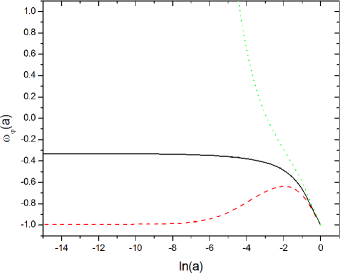
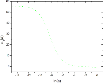
Figure 1: (a) Equation of state parameter of the holographic quintessence model, for $c=0.85$ and $\delta M_{Pl}=-0.1$ (red dashed line), $\delta M_{Pl}=0$ (black solid line) and $\delta M_{Pl}=+0.1$ (green dotted line). (b) Full range of the equation of state parameter for $\delta M_{Pl}=+0.1$.

In figure 2, $V(\varphi)$ is shown for some values of $\delta$ and $c$. Notice that there is a region where $V(\varphi)$ is almost constant, that is, there is a slow-roll region. As we chose $\dot{\varphi}$ positive, then $\varphi$ evolves to this slow-roll region. However, if we had chosen $\dot{\varphi}$ negative, then because the right hand side of (25) would have the opposite sign, so $\frac{dV(\varphi)}{d\varphi}$ would have also the opposite sign and again $\varphi$ would evolve to the slow-roll region. Notice also that for $\delta M_{Pl}=+0.1$, the potential is negative in the past.

The equation for evolution of $\varphi$ (25) can be written in an integral form as

$$\Delta\varphi\left(z\right)=-\sqrt{3}M_{Pl}\int_{0}^{z}\frac{\sqrt{\Omega_{\varphi}(z)\left(1+\omega_{\varphi}\left(z\right)\right)}}{1+z}dz\text{ .}$$

Since the model depends on $\Delta\varphi$ - through $E\left(z\right)$ - and neither on $\varphi$ nor on $\varphi_{0}$, then it is independent of $\varphi_{0}$. In other words, $\varphi_{0}$ is not a parameter of the model and can be chosen arbitrarily. Therefore, the parameters of the model are $\delta$, $c$, $h,$ $\Omega_{b0}$ and $\Omega_{\varphi 0}$.

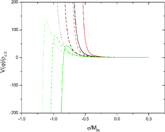
Figure 2: Potential of the holographic quintessence field $V(\varphi)$, in units of $\rho_{c0}=3M_{Pl}^{2}H_{0}^{2}$. $\varphi$ is in units of $M_{Pl}$. The solid lines are for $c=0.95$, the dashed ones are for $c=1.1$ and the dotted are for $c=1.25$. For each value of $c$ the curves from right to left are for $\delta M_{Pl}=-0.1$ (red), $\delta M_{Pl}=0$ (black) and $\delta M_{Pl}=+0.1$ (green), respectively.

II.2 Tachyon scalar field

In the case of dark energy modeled as the tachyon scalar field, $\mathcal{L}_{\varphi}\left(x\right)$ in the action (1) is given by (4). From a variational principle, we obtain

$$i\gamma^{\mu}\nabla_{\mu}\Psi-M^{\ast}\Psi=0\text{ ,}$$ (27)

$$i(\nabla_{\mu}\bar{\Psi})\gamma^{\mu}+M^{\ast}\bar{\Psi}=0\text{ ,}$$ (28)

where $M^{\ast}\equiv M-\beta\varphi$, and

$$\nabla_{\mu}\partial^{\mu}\varphi+\alpha\frac{\partial^{\mu}\varphi(\nabla_{\mu}\partial_{\sigma}\varphi)\partial^{\sigma}\varphi}{1-\alpha\partial_{\mu}\varphi\partial^{\mu}\varphi}+\frac{1}{\alpha}\frac{dlnV(\varphi)}{d\varphi}=\frac{\beta\bar{\Psi}\Psi}{\alpha V(\varphi)}\sqrt{1-\alpha\partial^{\mu}\varphi\partial_{\mu}\varphi}\text{ .}$$ (29)

The equations of motion for $\Psi$ and $\bar{\Psi}$ (27) and (28) are the interacting covariant Dirac equation and its adjoint, respectively, i. e., (27) and (28) are almost the same as eqs. (5) and (6), the only difference is that the scalar field $\varphi$ in $M^{\ast}$ now is the tachyon field. For homogeneous fields and adopting the Friedmann-Robertson-Walker metric, $g_{\mu\nu}$=diag$\left(1,-a^{2}\left(t\right),-a^{2}\left(t\right),-a^{2}\left(t\right)\right)$, where $a^{2}\left(t\right)$ is the scale factor, (29) reduces to

$$\ddot{\varphi}=-(1-\alpha\dot{\varphi}^{2})\left[\frac{1}{\alpha}\frac{dlnV(\varphi)}{d\varphi}+3H\dot{\varphi}-\frac{\beta\bar{\Psi}\Psi}{\alpha V(\varphi)}\sqrt{1-\alpha\dot{\varphi}^{2}}\right]\text{ ,}$$ (30)

whereas for the fermions, the equations of motion will reduce to eq. (8), as already obtained above:

$$\bar{\Psi}\Psi=\bar{\Psi}_{0}\Psi_{0}\left(\frac{a_{0}}{a}\right)^{3}\text{ .}$$ (8)

From the energy-momentum tensor, we get

$$\rho_{\varphi} =\frac{V(\varphi)}{\sqrt{1-\alpha\dot{\varphi}^{2}}}\text{ ,}$$ (31)

$$P_{\varphi} =-V(\varphi)\sqrt{1-\alpha\dot{\varphi}^{2}}\text{ ,}$$ (32)

$$\rho_{\Psi} =M^{\ast}\bar{\Psi}\Psi\text{ ,}$$

$$P_{\Psi} =0\text{ .}$$

From (31) and (32) we have $\omega_{\varphi}\equiv\frac{P_{\varphi}}{\rho_{\varphi}}=\alpha\dot{\varphi}^{2}-1$. Deriving (31) and (32) with respect to time and using (30) and (8), we get

$$\dot{\rho}_{\varphi}+3H\rho_{\varphi}(\omega_{\varphi}+1)=\beta\dot{\varphi}\bar{\Psi}_{0}\Psi_{0}\left(\frac{a_{0}}{a}\right)^{3}$$ (33)

and

$$\dot{\rho}_{\Psi}+3H\rho_{\Psi}=-\beta\dot{\varphi}\bar{\Psi}_{0}\Psi_{0}\left(\frac{a_{0}}{a}\right)^{3}\text{ ,}$$ (34)

where the dot represents derivative with respect to time.

For baryonic matter and radiation, the conservation equations are the same as in the quintessence model. We have

$$\dot{\rho}_{b}+3H\rho_{b}=0$$ (15)

and

$$\dot{\rho}_{r}+3H\rho_{r}(\omega_{r}+1)=0\text{ ,}$$ (16)

where $\omega_{r}=\frac{1}{3}$. Eqs. (15) and (16) implies that $\rho_{b}=\frac{\rho_{b0}}{a^{3}}$ and $\rho_{r}=\frac{\rho_{r0}}{a^{4}}$, respectively. The subscript $0$ denotes the quantities today. We are considering the radiation as composed by photons and massless neutrinos, so that $\rho_{r0}=\left(1+0.2271N_{eff}\right)\rho_{\gamma 0}$, where $N_{eff}=3.04$ is the effective number of relativistic degrees of freedom and $\rho_{\gamma 0}$ is the energy density of photons, given by $\rho_{\gamma 0}=\frac{\pi^{2}}{15}T_{CMB}$, being $T_{CMB}=2.725K$ the CMB temperature today. The Friedmann equation for a flat universe reads

$$H^{2}=\frac{1}{3M_{Pl}^{2}}\left[M^{\ast}\bar{\Psi}_{0}\Psi_{0}\left(\frac{a_{0}}{a}\right)^{3}+\frac{V(\varphi)}{\sqrt{1-\alpha\dot{\varphi}^{2}}}+\frac{\rho_{b0}}{a^{3}}+\frac{\rho_{r0}}{a^{4}}\right]\text{ .}$$ (35)

Now, as done in the case of the quintessence field, we will identify the tachyon energy density (31) with the holographic dark energy density $\rho_{\Lambda}=3c^{2}M_{Pl}^{2}L^{-2}$. From a similar reasoning, we obtain again the equations (18), (19) and (20),

$$\frac{d\Omega_{\varphi}}{dz}=-\frac{\Omega_{\varphi}}{1+z}\left(2\frac{\sqrt{\Omega_{\varphi}}}{c}+3\Omega_{\varphi}\omega_{\varphi}+\Omega_{r}+1\right)\text{ ,}$$ (18)

$$\frac{d\Omega_{b}}{dz}=-\frac{\Omega_{b}}{1+z}\left(3\Omega_{\varphi}\omega_{\varphi}+\Omega_{r}\right)$$ (19)

and

$$\frac{d\Omega_{r}}{dz}=-\frac{\Omega_{r}}{1+z}\left(3\Omega_{\varphi}\omega_{\varphi}+\Omega_{r}-1\right)\text{ .}$$ (20)

Also we obtain

$$\dot{r}=3Hr\omega_{\varphi}-sign\left[\dot{\varphi}\right]\frac{\beta\left(1+r\right)^{2}\sqrt{1+\omega_{\varphi}}}{3M_{Pl}^{2}\sqrt{\alpha}H^{2}}\bar{\Psi}_{0}\Psi_{0}\left(\frac{1+z}{1+z_{0}}\right)^{3}\text{ ,}$$ (36)

with $r\equiv\frac{\rho_{\Psi}}{\rho_{\varphi}}$. The sign of $\dot{\varphi}$ is arbitrary, as it can be modified by redefinitions of the field, $\varphi\rightarrow-\varphi$, and of the coupling constant, $\beta\rightarrow-\beta$. We can rewrite $\bar{\Psi}_{0}\Psi_{0}$ in terms of observable quantities, by imposing that the dark matter density today matches the observed value. We obtain $M\bar{\Psi}_{0}\Psi_{0}=\frac{3M_{Pl}^{2}H_{0}^{2}\left(1-\Omega_{\phi 0}-\Omega_{b0}-\Omega_{r0}\right)}{1-\frac{\beta}{M\sqrt{\alpha}}\phi_{0}}$, where we defined $\phi\equiv\sqrt{\alpha}\varphi$. Furthermore, noticing that $r=\frac{1-\Omega_{\varphi}-\Omega_{b}-\Omega_{r}}{\Omega_{\varphi}}$, we can eliminate $r$ and $\dot{r}$ in favor of $\Omega_{\varphi}$, $\Omega_{b}$, $\Omega_{r}$, $\dot{\Omega}_{\varphi}$, $\dot{\Omega}_{b}$ and $\dot{\Omega}_{r}$ in (36). Using (18), (19) and (20) we obtain, after some algebra

$$\omega_{\phi}\left(z\right)=-\frac{1}{3}-\frac{2\sqrt{\Omega_{\phi}\left(z\right)}}{3c}+\frac{\gamma\left(z\right)}{3}\left[\gamma\left(z\right)+\sqrt{\gamma\left(z\right)^{2}+4\left(1-\frac{\sqrt{\Omega_{\phi}\left(z\right)}}{c}\right)}\right]\text{ ,}$$ (37)

where

$$\gamma\left(z\right)\equiv\frac{1}{\sqrt{6}}\frac{\delta}{H_{0}}\frac{1-\Omega_{\phi 0}-\Omega_{b0}-\Omega_{r0}}{\Omega_{\phi}\left(z\right)E^{3}\left(z\right)}\left(\frac{1+z}{1+z_{0}}\right)^{3}\text{ ,}$$ (38)

with

$$E\left(z\right)\equiv\frac{H\left(z\right)}{H_{0}}=\sqrt{\frac{\left[\left(1-\delta\Delta\phi\right)\left(1-\Omega_{\phi 0}-\Omega_{b0}-\Omega_{r0}\right)+\Omega_{b0}\right]}{1-\Omega_{\phi}}\left(\frac{1+z}{1+z_{0}}\right)^{3}+\frac{\Omega_{r0}}{1-\Omega_{\phi}}\left(\frac{1+z}{1+z_{0}}\right)^{4}}\text{ ,}$$ (39)

where $\Delta\phi\left(z\right)\equiv\phi\left(z\right)-\phi_{0}$ and $\delta\equiv\frac{\frac{\beta}{M\sqrt{\alpha}}}{1-\frac{\beta}{M\sqrt{\alpha}}\phi_{0}}$ is an effective coupling constant. As in the quintessence field case, if $\delta=0$, (37) reproduces the equation of state parameter obtained in Li .

The evolution of the tachyon scalar field is given by

$$\frac{d\phi}{dz}=-\frac{\sqrt{1+\omega_{\phi}\left(z\right)}}{H_{0}E\left(z\right)\left(1+z\right)}\text{ .}$$ (40)

From (18), (19), (20) and (40) we can calculate the evolution with redshift of all observables in the model. If we wish to calculate the time dependence, we need to integrate the Friedmann equation (35), which can be written in the form

$$\frac{dt}{dz}=-\frac{1}{H_{0}E(z)(1+z)}\text{ .}$$

From (31), we can compute the potential $V\left(z\right)$ as

$$\frac{V\left(z\right)}{\rho_{c0}}=E^{2}\left(z\right)\Omega_{\phi}\left(z\right)\sqrt{-\omega_{\phi}\left(z\right)}\text{ ,}$$ (41)

where $\rho_{c0}=3M_{Pl}^{2}H_{0}^{2}$, $E\left(z\right)$ is given by (39), $\omega_{\phi}\left(z\right)$ is given by (37) and $\Omega_{\phi}\left(z\right)$ is the solution of (18). From (41) and (40), we can compute $V(\phi)$.

The square root in (37) must be real. Furthermore, in analogous manner to the quintessence model, $\omega_{\phi}$ must be more than $-1$ because (40). We can verify that $\omega_{\phi}$ is real and $\omega_{\phi}>-1$ if (i) $\frac{\sqrt{\Omega_{\phi 0}}}{c}<1$ or (ii) $\frac{\sqrt{\Omega_{\phi 0}}}{c}>1$ and $\frac{\left|\delta\right|}{H_{0}}>2\sqrt{6}\frac{\Omega_{\phi 0}}{1-\Omega_{\phi 0}-\Omega_{b0}-\Omega_{r0}}\sqrt{\frac{\sqrt{\Omega_{\phi 0}}}{c}-1}$. However, case (ii) is irrelevant, as it corresponds to large values of $\frac{\left|\delta\right|}{H_{0}}$. For example, if $\Omega_{\phi 0}=0.7$ and $c=0.8$, we have $\frac{\left|\delta\right|}{H_{0}}\gtrsim 2.45$. Below, we will see that the observational data constrain $\frac{\left|\delta\right|}{H_{0}}\sim 10^{-1}$. In order that $\omega_{\phi}$ be real for all future times, as $\Omega_{\phi}\rightarrow 1$, it is necessary that $c\geq 1$. As already mentioned in the quintessence case, this is also the condition for the entropy to increase for all future times, so the tachyon model also respects the second law of thermodynamics.

The evolution of the equation of state parameter $\omega_{\phi}$ is showed in figure 3. We have $\omega_{\phi}\rightarrow-1/3$ for $z\gg 1$. In the non interacting case - $\delta=0$ - this occurs simply because $\Omega_{\phi}(z)\ll 1$ in high redshifts. The behaviour for the interacting case - $\delta\neq 0$ - is explained as follows. In the matter era $E^{2}(z)\sim\left(1+z\right)^{3}$ so that $\gamma\left(z\right)\sim\frac{1}{\Omega_{\phi}\left(z\right)\left(1+z\right)^{1,5}}$. Using (18) we infer $\frac{d\left|\gamma\left(z\right)\right|}{dz}>0$, that is $\left|\gamma\left(z\right)\right|$ increases with redshift $z$. Therefore, if $\delta<0$ then $\gamma\left(z\right)<0$ and $\omega_{\phi}$ increases slower than in the non interacting case. If $\delta>0$ then $\gamma\left(z\right)>0$ and $\omega_{\phi}$ increases faster than in the non interacting case. In the radiation era $\gamma\left(z\right)\sim\frac{1}{1+z}$ and it turns out to be negligible, so that $\omega_{\phi}\simeq-1/3$.

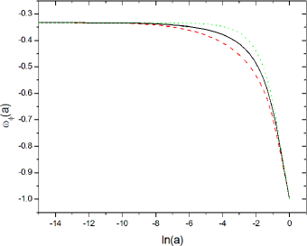
Figure 3: Equation of state parameter of the holographic tachyon model, for $c=0.85$ and $\frac{\delta}{H_{0}}=-0.1$ (red dashed line), $\frac{\delta}{H_{0}}=0$ (black solid line) and $\frac{\delta}{H_{0}}=+0.1$ (green dotted line).

In figure 4, $V(\phi)$ is shown for some values of $\delta$ and $c$. Notice that - as in the case of the quintessence field potential - there is a region where $V(\phi)$ is almost constant, that is, there is a slow-roll region. As we chose $\dot{\phi}$ positive, then $\phi$ evolves to this slow-roll region. However, if we had chosen $\dot{\phi}$ negative, then because the right hand side of (40) would have the opposite sign, so $\frac{dV(\phi)}{d\phi}$ would have also the opposite sign and again $\phi$ would evolve to the slow-roll region.

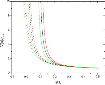
Figure 4: Potential of the holographic tachyon field $V(\phi)$, in units of $\rho_{c0}=3M_{Pl}^{2}H_{0}^{2}$. $\phi$ is in units of $H_{0}^{-1}$. The solid lines are for $c=0.85$, the dashed ones are for $c=1.1$ and the dotted are for $c=1.35$. For each value of $c$ the curves from right to left are for $\frac{\delta}{H_{0}}=-0.1$ (red), $\frac{\delta}{H_{0}}=0$ (black) and $\frac{\delta}{H_{0}}=+0.1$ (green), respectively.

The equation for evolution of $\phi$ (40) can be written in an integral form as

$$\Delta\phi=-\frac{1}{H_{0}}\int_{0}^{z}\frac{\sqrt{1+\omega_{\phi}\left(z\right)}}{E(z)(1+z)}dz\text{ .}$$

As before, the model depends on $\Delta\phi$ - through $E\left(z\right)$ - and neither on $\phi$ nor on $\phi_{0}$, then it is independent of $\phi_{0}$. Therefore, the parameters of the model are $\delta$, $c$, $h,$ $\Omega_{b0}$ and $\Omega_{\phi 0}$. Below, we discuss the comparison with observational data and the results obtained.

III Constraints from observational data

In lookback , the lookback time method has been discussed. Given an object $i$ at redshift $z_{i}$, its age $t(z_{i})$ is defined as the difference between the age of the universe at $z_{i}$ and the age of the universe at the formation redshift of the object, $z_{F}$, that is,

$$t(z_{i}) =H_{0}^{-1}\left[\int_{z_{i}}^{\infty}\frac{dz^{\prime}}{(1+z^{\prime})E(z^{\prime})}-\int_{z_{F}}^{\infty}\frac{dz^{\prime}}{(1+z^{\prime})E(z^{\prime})}\right]$$

$$=H_{0}^{-1}\int_{z_{i}}^{z_{F}}\frac{dz^{\prime}}{(1+z^{\prime})E(z^{\prime})}=t_{L}(z_{F})-t_{L}(z_{i})\text{ ,}$$ (42)

where $t_{L}$ is the lookback time, given by

$$t_{L}(z)=H_{0}^{-1}\int_{0}^{z}\frac{dz^{\prime}}{(1+z^{\prime})E(z^{\prime})}\text{ .}$$

Using (42), the observational lookback time $t_{L}^{obs}(z_{i})$ is

$$t_{L}^{obs}(z_{i}) =t_{L}(z_{F})-t(z_{i})=[t_{0}^{obs}-t(z_{i})]-[t_{0}^{obs}-t_{L}(z_{F})]$$

$$=t_{0}^{obs}-t(z_{i})-df\text{ ,}$$ (43)

where $t_{0}^{obs}$ is the estimated age of the universe today and $df$ is the delay factor,

$$df\equiv t_{0}^{obs}-t_{L}(z_{F})\ .$$

We now minimize $\chi_{lbt}^{2}$,

$$\chi_{lbt}^{2}=\sum_{i=1}^{N}\frac{[t_{L}(z_{i},\vec{p})-t_{L}^{obs}(z_{i})]^{2}}{\sigma_{i}^{2}+\sigma_{t_{0}^{obs}}^{2}}\text{ ,}$$

where $t_{L}(z_{i},\vec{p})$ is the theoretical value of the lookback time in $z_{i}$, $\vec{p}$ denotes the theoretical parameters, $t_{L}^{obs}(z_{i})$ is the corresponding observational value given by (43), $\sigma_{i}$ is the uncertainty in the estimated age $t(z_{i})$ of the object at $z_{i}$, which appears in (43) and $\sigma_{t_{0}^{obs}}$ is the uncertainty in getting $t_{0}^{obs}$. The delay factor $df$ appears because of our ignorance about the redshift formation $z_{F}$ of the object and has to be adjusted. Note, however, that the theoretical lookback time does not depend on this parameter, and we can marginalize over it.

In age35 and age32 the ages of 35 and 32 red galaxies are respectively given. For the age of the universe one can adopt $t_{0}^{obs}=13.75\pm 0.11Gyr$ wmap7yr . Although this estimate for $t_{0}^{obs}$ has been obtained assuming a $\Lambda CDM$ universe, it does not introduce systematical errors in the calculation: any systematical error eventually introduced here would be compensated by the adjust of $df$, in (43). On the other hand, such an estimate is in perfect agreement with other estimates, which are independent of the cosmological model, as for example $t_{0}^{obs}=12.6_{-2.4}^{+3.4}Gyr$, obtained from globular cluster ages krauss and $t_{0}^{obs}=12.5\pm 3.0Gyr$, obtained from radioisotopes studies cayrel .

The WMAP distance information used by the WMAP colaboration includes the “shift parameter” $R$, the “acoustic scale” $l_{A}$ and the redshift of decoupling $z_{\ast}$. These quantities are very weakly model dependent liR . $R$ and $l_{A}$ are given by

$$R=\sqrt{\Omega_{m0}}H_{0}r\left(z_{\ast}\right)$$

and

$$l_{A}=\pi\frac{r\left(z_{\ast}\right)}{r_{s}\left(z_{\ast}\right)}\text{ ,}$$

where $r\left(z_{\ast}\right)$ is the comoving distance to $z_{\ast}$ and $r_{s}\left(z_{\ast}\right)$ is the comoving sound horizon at $z_{\ast}$. For a flat universe, $r\left(z_{\ast}\right)$ and $r_{s}\left(z_{\ast}\right)$ are given by

$$r\left(z_{\ast}\right)=\frac{1}{H_{0}}\int_{0}^{z_{\ast}}\frac{dz}{E(z)}$$

and

$$r_{s}\left(z_{\ast}\right)=\frac{1}{H_{0}}\int_{0}^{z_{\ast}}\frac{dz}{E(z)\sqrt{3\left(1+\bar{R}_{b}/(1+z)\right)}}\text{ ,}$$

where $\bar{R}_{b}=3\Omega_{b0}/\left(4\Omega_{\gamma 0}\right)$. For the redshift of decoupling $z_{\ast}$ we use the fitting function proposed by Hu and Sugiyama sugiyama :

$$z_{\ast}=1048\left[1+0.00124\left(\Omega_{b0}h^{2}\right)^{-0.738}\right]\left[1+g_{1}\left(\Omega_{m0}h^{2}\right)^{g_{2}}\right]\text{ ,}$$

where

$$g_{1}=\frac{0.0783\left(\Omega_{b0}h^{2}\right)^{-0.238}}{1+39.5\left(\Omega_{b0}h^{2}\right)^{0.763}}$$

and

$$g_{2}=\frac{0.560}{1+21.1\left(\Omega_{b0}h^{2}\right)^{1.81}}\text{ .}$$

Thus we add to $\chi^{2}$ the term

$$\chi_{CMB}^{2}={\displaystyle\sum\limits_{ij}}\left(x_{i}^{th}-x_{i}^{data}\right)\left(C^{-1}\right)_{ij}\left(x_{j}^{th}-x_{j}^{data}\right)\text{ ,}$$

where $x=\left(l_{A},R,z_{\ast}\right)$ is the parameter vector and $\left(C^{-1}\right)_{ij}$ is the inverse covariance matrix for the seven-year WMAP distance information wmap7ykomatsu .

Baryonic Acoustic Oscilations (BAO) are described in terms of the parameter

$$A=\sqrt{\Omega_{M}}E(z_{BAO})^{-1/3}\left[\frac{1}{z_{BAO}}\int_{0}^{z_{BAO}}\frac{dz^{\prime}}{E(z^{\prime})}\right]^{2/3}\text{ ,}$$

where $z_{BAO}=0.35$. It has been estimated that $A_{obs}=0.493\pm 0.017$ BAO1 . We thus add to $\chi^{2}$ the term

$$\chi_{BAO}^{2}=\frac{\left(A-A_{obs}\right)^{2}}{\sigma_{A}^{2}}\ \text{.}$$

The BAO distance ratio $r_{BAO}\equiv D_{V}\left(z=0.35\right)/D_{V}\left(z=0.20\right)=1.812\pm 0.060$, estimated from the joint analysis of the 2dFGRS (Two Degree Field Galaxy Redshift Survey) and SDSS (Sloan Digital Sky Survey) data BAO2 , has also been included. It was demonstrated in BAO2 that this quantity is weakly model dependent. The quantity $D_{V}\left(z_{BAO}\right)$ is given by

$$D_{V}\left(z_{BAO}\right)=c\left[\frac{z_{BAO}}{H\left(z_{BAO}\right)}\left(\int_{0}^{z_{BAO}}\frac{dz^{\prime}}{H\left(z^{\prime}\right)}\right)^{2}\right]^{1/3}\text{ .}$$

So we have the contribution

$$\chi_{r_{BAO}}^{2}=\frac{\left(r_{BAO}-r_{BAO}^{obs}\right)^{2}}{\sigma_{r_{BAO}}^{2}}\text{ .}$$

Finally, we add the 397 supernovae data from Constitution compilation constitution . Defining the distance modulus

$$\mu(z)=5log_{10}\left[c(1+z)\int_{0}^{z}\frac{dz^{\prime}}{E(z^{\prime})}\right]+25-5log_{10}H_{0}\text{ ,}$$

we have the contribution

$$\chi_{SN}^{2}=\sum_{j=1}^{397}\frac{[\mu(z_{j})-\mu_{obs}(z_{j})]^{2}}{\sigma_{j}^{2}}\text{ .}$$

Using the expression $\chi^{2}=\chi_{lbt}^{2}+\chi_{CMB}^{2}+\chi_{BAO}^{2}+\chi_{r_{BAO}}^{2}+\chi_{SN}^{2}$, the likelihood function is given by

$$\mathcal{L}(\delta,c,h,\Omega_{b0},\Omega_{\phi_{0}})\propto exp[-\frac{\chi^{2}(\delta,c,h,\Omega_{b0},\Omega_{\phi_{0}})}{2}]\ \text{.}$$

III.1 Quintessence field

In table 1 we present the values of the individual best fit parameters, with respective $1\sigma$, $2\sigma$ and $3\sigma$ confidence intervals.

Table 1: Values of the holographic quintessence model parameters from lookback time, CMB, BAO and SNe Ia. In the last line, $\chi_{\min}^{2}/dof$ is the minimum $\chi^{2}$ per degree of freedom.

$\delta M_{Pl}$	$-0.170_{-0.072-0.123-0.225}^{+0.067+0.148.+0.187}$
$c$	$0.891_{-0.016-0.028-0.035}^{+0.048+0.134+0.234}$
$\Omega_{\phi 0}$	$0.7733_{-0.0087-0.0217-0.0353}^{+0.0092+0.0162+0.0264}$
$\Omega_{b0}$	$0.0450_{-0.0028-0.0048-0.0066}^{+0.0026+0.0061+0.0089}$
$h$	$0.687\pm 0.013\pm 0.026\pm 0.039$
$\chi_{\min}^{2}/dof$	$1.185$

Figure 5 shows the marginalized probability distributions for $\delta$ and $c$. The coupling constant $\delta$ is non vanishing at $2\sigma$ confidence level. Figure 6 shows some joint confidence regions of two parameters. Notice the effect of the condition $\omega_{\phi}\leq 1$ on the positive tail of the probability distribuction of $\delta$ and also in the confidence regions of $\delta$ with other parameters.

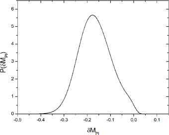
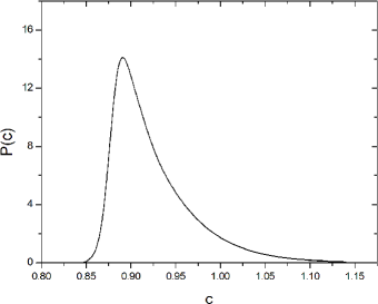
Figure 5: Probability distribuctions of the coupling constant $\delta$ (left panel) and of the parameter $c$ (right panel) of the holographic quintessence model.

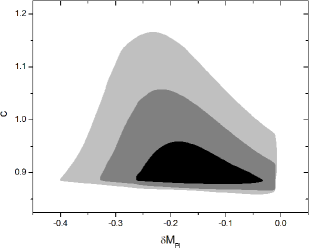
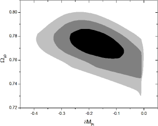
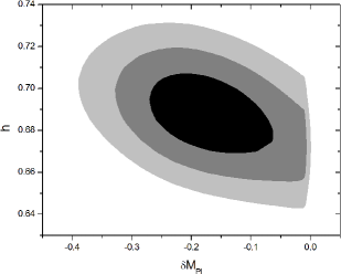
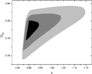
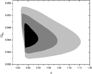
Figure 6: Two parameters confidence regions of $1\sigma$, $2\sigma$ and $3\sigma$ of the holographic quintessence model.

III.2 Tachyon scalar field

In table 2 we present the values of the individual best fit parameters, with respective $1\sigma$, $2\sigma$ and $3\sigma$ confidence intervals.

Table 2: Values of the holographic tachyon model parameters from lookback time, CMB, BAO and SNe Ia. In the last line, $\chi_{\min}^{2}/dof$ is the minimum $\chi^{2}$ per degree of freedom.

$\frac{\delta}{H_{0}}$	$-0.201_{-0.059-0.138-0.249}^{+0.063+0.117+0.176}$
$c$	$0.868_{-0.020-0.030-0.038}^{+0.059+0.165+0.235}$
$\Omega_{\phi 0}$	$0.724_{-0.012-0.026-0.040}^{+0.013+0.025+0.036}$
$\Omega_{b0}$	$0.0480\pm 0.0021\pm 0.0041\pm 0.0062$
$h$	$0.669\pm 0.012\pm 0.025\pm 0.037$
$\chi_{\min}^{2}/dof$	$1.148$

Figure 7 shows the marginalized probability distributions for $\delta$ and $c$. The coupling constant $\delta$ is non vanishing at more than $3\sigma$ confidence level. So for this model we obtained strong evidence for interaction. Figure 8 shows some confidence regions of two parameters for this model.

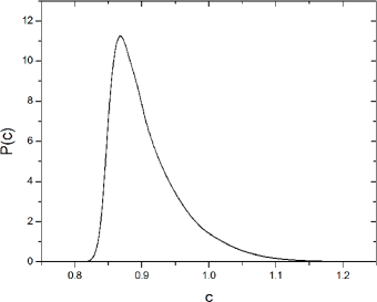
Figure 7: Probability distribuctions of the coupling constant $\delta$ (left panel) and of the parameter $c$ (right panel) of the holographic tachyon model.

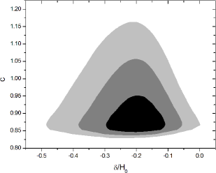
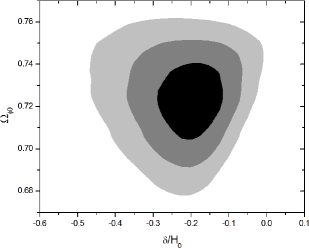
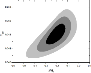
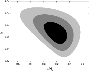
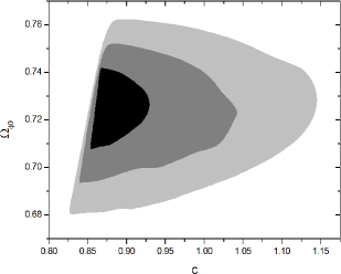
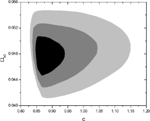
Figure 8: Two parameters confidence regions of $1\sigma$, $2\sigma$ and $3\sigma$ of the holographic tachyon model.

IV Discussion and conclusions

The minimum $\chi^{2}$ per degree of freedom values indicate that both models fit well the observational data. Moreover, we see that the tachyon model is a bit more favored by the observational data than the quintessence one. The dimensionless coupling constants, $\delta M_{Pl}$ for the quintessence field and $\frac{\delta}{H_{0}}$ for the tachyon, agree at $1\sigma$ level and for both models we obtained significative evidence for a non vanishing interaction in the dark sector. Furthermore, both the results implies in dark energy decaying into dark matter, alleviating the coincidence problem. These results are consistent with previous ones, as for example those obtained in sandro2 , where an interacting tachyonic dark energy model with a power law potential was assumed and the results were consistent with the interaction at $90\%$ confidence level. We must also mention that in sandro and virial evidence for interaction was found using completely different models and data sets. So those results combined with the present ones furnish sensible evidence in favor of an interaction in the dark sector of the universe.

The results obtained for $c$, $\Omega_{b0}$ and $h$ for the two models also agree at $1\sigma$ confidence level. The values obtained for $\Omega_{\phi 0}$ agree only at $2\sigma$ level. For the quintessence model, $\Omega_{\phi 0}$ is almost superestimated, corresponding to a matter relative density today $\Omega_{m0}=0.231\pm 0.010$. This value agrees at inferior limit of $1\sigma$ with the cosmological model independent estimative $\Omega_{Mobs}=0.28\pm 0.04$ riess . For the tachyon model, $\Omega_{\phi 0}$ corresponds to a matter relative density today $\Omega_{m0}=0.276_{-0.012}^{+0.013}$, which is in perfect agreement with that observational estimative. For both models, the baryionic density and the Hubble parameter today are very reasonable. We have obtained $\Omega_{b0}h^{2}=0.0212\pm 0.0015$ and $\Omega_{b0}h^{2}=0.0215\pm 0.0012$ from quintessence and tachyon models, respectively. Let’s compare these values, for example, with that obtained from deuterium to hydrogen abundance ratio omeara , $\Omega_{b0}h^{2}=0.0213\pm 0.0013\pm 0.0004$, where the errors terms represents the $1\sigma$ errors from deuterium to hydrogen abundance ratio and the uncertainties in the nuclear reaction rates, respectively. For the Hubble parameter, we have obtained $h=0.687\pm 0.013$ and $h=0.669\pm 0.012$ from the quintessence and tachyon models, respectively, both in excellent agreement with observational values, independent of cosmological model, as for example $h_{obs}=0.69\pm 0.12$ age35 and $h_{obs}=0.72\pm 0.08$ key . We can also compare the ratios $\Omega_{b0}/\Omega_{m0}=0.248_{-0.023}^{+0.022}$, from the quintessence model, and $\Omega_{b0}/\Omega_{m0}=0.211\pm 0.016$, from the tachyon model, with the observational value of 2dFGRS colaboration, $\Omega_{b0}/\Omega_{m0}=0.185\pm 0.046$ 2dFGRS .

We have obtained $c<1$ at $1\sigma$ confidence level for both models. As already said above, this implies that the equation of state parameter $\omega_{\phi}$ will not be real for all future times. However, this is not a very serious problem, because $c$ is compatible with values above unit at $2\sigma$ confidence level. Moreover, one could say that $c<1$ is only an effect due to lack of more precise observational data. Anyway, the very simple models presented here are expected to be only alternatives to an effective description of a more sophisticated subjacent theory of dark energy. In principle, nothing guarantees that they will be good descriptions for all future times.

Figures 6 and 8 shows some joint confidence regions of two parameters for both models. In the confidence regions for $\delta$ versus $c$ and for $c$ versus $\Omega_{\phi 0}$, we see that there is a lower limit on $c$ $\approx 0.8$. This also can be seen in the marginalized probability distributions of $c$, which dies for $c\lesssim 0.85$. This lower limit is explained by the condition $\frac{\sqrt{\Omega_{\phi 0}}}{c}<1$, necessary for $\omega_{\phi}$ to be real and $\omega_{\phi}>-1$, discussed above. This limit can be seen more clearly in $c$ versus $\Omega_{\phi 0}$ confidence regions. Moreover, we have $c\simeq\sqrt{\Omega_{\phi 0}}$ for the best fit values of these parameters. This implies that $\omega_{\phi 0}\simeq-1$ and both models approaches $\Lambda CDM$ today. This is consistent with the fact that, as $\Lambda CDM$ fits all observational data, then any alternative model must not deviates much from $\Lambda CDM$ for $z\approx 0$. However, for $z>0$, both models are qualitatively different from $\Lambda CDM$. For the quintessence field we have very different qualitative behaviours for $\delta<0$, $\delta=0$ and $\delta>0$, as showed in figure 1 and discussed in II A. For the tachyon model its behaviour is qualitatively the same in the three cases, $\omega_{\phi}$ approximates $-1/3$, as showed in figure 3 and discussed in II B.

It is interesting to compare the results obtained in the present work for the holographic tachyon model with the previous ones, presented in sandro3 , where a simpler version of the holographic tachyon model, without barions nor radiation, had been compared with observational data. The values obtained here for $c,$ $\Omega_{\phi 0}$ and $h$ are the same as before and with minor incertainty intervals, despite the fact that here we have one more parameter - $\Omega_{b0}$ -, as we can see by comparing table 2 in the present work with table 1 in sandro3 . This is because now it was possible to use all WMAP distance information $R,$ $l_{A}$ and $z_{\ast}$, as the model was generalized to include barions and radiation. However the dark energy coupling constant $\delta$ now is non vanishing and compatible with dark energy decaying into dark matter with more than $3\sigma$ confidence level, whereas in sandro3 no evidence of interaction had been found. This can be understood as follows. In low redshifts, the universe is dominated by dark energy. The dynamics of dark energy in low redshifts is essentially determined by the equation of state parameter $\omega_{\phi}\left(z\right)$, as can be seen in (18). As in this period the data sets were the same in both the works, so $\omega_{\phi}\left(z\right)$ must be almost the same in this period in both the works. But $\omega_{\phi}\left(z\right)$ explicitly depends on the product $\delta\Omega_{\Psi 0}$, were $\delta$ is the coupling constant and $\Omega_{\Psi 0}=1-\Omega_{\varphi 0}-\Omega_{b0}-\Omega_{r0}$ is the dark matter relative density, as we can see in (37) and (38). As in the present work $\Omega_{\Psi 0}$ is less than that in sandro3 - where $\Omega_{b0}=\Omega_{r0}\equiv 0$ -, it turns out that $\delta$ in the present work is bigger (in modulus) than that in sandro3 . However it is important to point out that in sandro3 the model was less realistic, as it wasn’t include barions nor radiation. Therefore, the present result favorable to interaction is more robust.

In summary, combinations of holographic dark energy model and scalar fields were implemented. It was showed that it is possible to fix the potential of interacting scalar fields by imposing that the energy density of the scalar field must match the energy density of the holographic dark energy. A comparison of the models with recent observational data was made and the coupling is non vanishing at more than $2\sigma$ for the quintessence field and at more than $3\sigma$ for the tachyon. In both cases the results are consistent with dark energy decaying into dark matter, alleviating the coincidence problem.

Acknowledgements

This work has been supported by CNPq (Conselho Nacional de Desenvolvimento Científico e Tecnológico) of Brazil.

References

- (1) W. Zimdahl and D. Pavon Phys. Lett. B521 (2001) 133; L. P. Chimento, A. S. Jakubi, D. Pavon and W. Zimdahl Phys. Rev. D67 (2003) 083513.
- (2) J.-H. He and B. Wang JCAP 06 (2008) 010; C. Feng, B. Wang, E. Abdalla and R.-K. Su Phys. Lett. B665 (2008) 111; J.-H. He, B. Wang and E. Abdalla, Phys. Lett. B671 (2009), 139.
- (3) B. Wang, J. Zang, C.-Y. Lin, E. Abdalla and S. Micheletti, Nucl. Phys. B778 (2007) 69.
- (4) S. Micheletti, E. Abdalla and B. Wang, Phys. Rev. D79 (2009) 123506.
- (5) B. Gumjudpai, T. Naskar, M. Sami and S. Tsujikawa JCAP 06 (2005) 007; B. Wang, Y.-G. Gong and E. Abdalla, Phys. Lett. B624 (2005) 141; M. R. Setare, Phys. Lett. B642 (2006) 1; Eur. Phys. J. C50 (2007) 991; idem, Phys. Lett. B654 (2007) 1; E. Abdalla and B. Wang Phys. Lett. B651 (2007) 89; R. Rosenfeld Phys. Rev. D75 (2007) 083509; M. Quartin, M. O. Calvao, S. E. Joras, R. R. R. Reis and I. Waga JCAP 05 (2008) 007; Q. Wu, Y. Gong, A. Wang and J.S. Alcaniz Phys. Lett. B659 (2008) 34; M.R. Setare and E. C. Vagenas Phys. Lett. B666 (2008) 111; M. Jamil, M. A. Rashid Eur. Phys. J. C56 (2008) 429; Eur. Phys. J. C58 (2008) 111; M.R. Setare and E. C. Vagenas, Int. J. Mod. Phys. D18 (2009) 147; X.-M. Chen, Y.-G. Gong and E. N. Saridakis,JCAP 04 (2009) 001; Z.-K. Guo, N. Ohta and S. Tsujikawa, Phys. Rev. D76 (2007) 023508; O. Bertolami, F. Gil Pedro and M. Le Delliou, Phys. Lett. B654 (2007) 165; O. Bertolami, F.Gil Pedro and M.Le Delliou, Gen. Rel. Grav. 41 (2009) 2839; L. P. Chimento, Phys. Rev. D81 (2010) 043525.
- (6) S. Micheletti, JCAP 05 (2010) 009.
- (7) P. J. E. Peebles, Physical Cosmology, (Princeton U. Press, 1993).
- (8) E. Abdalla, L. R. W. Abramo, L. Sodre Jr. and B. Wang, Phys. Lett. B673, (2009) 107; E. Abdalla, L. R. W. Abramo and J. C. C. de Souza, Phys. Rev. D82 (2010) 023508.
- (9) R. Bean, E. E. Flanagan, I. Laszlo and M. Trodden Phys. Rev. D78 (2008) 123514.
- (10) E. J. Copeland, M. Sami and S. Tsujikawa, Int. J. Mod. Phys. D15 (2006) 1753; M. Sami Curr. Sci. 97 (2009) 887.
- (11) I. Zlatev, L. Wang and P. J. Steinhardt, Phys. Rev. Lett. 82 (1999) 896; P. J. Steinhardt, L. Wang and I. Zlatev, Phys. Rev. D59 (1999) 123504; L. Amendola Phys. Rev. D62 (2000) 043511; R.R. Caldwell and E. V. Linder, Phys. Rev. Lett.95 (2005) 141301; R. J. Scherrer and A. A. Sen, Phys. Rev. D77 (2008) 083515; A. A. Sen, G. Gupta and S. Das, JCAP 09 (2009) 027.
- (12) A. Sen JHEP 04 (2002) 048; JHEP 07 (2002) 065; Mod. Phys. Lett. A17 (2002) 1797.
- (13) T. Padmanabhan Phys. Rev. D66 (2002) 021301; A. Feinstein Phys. Rev. D66 (2002) 063511; J. S. Bagla, H. K. Jassal and T. Padmanabhan Phys. Rev. D67 (2003) 063504; L. R. W. Abramo and F. Finelli Phys. Lett. B575 (2003) 165; R. Herrera, D. Pavon and W. Zimdahl, Gen. Rel. Grav. vol. 36 no 9 (2004) 2161; A. Ali, M. Sami and A. A. Sen, Phys. Rev. D79 (2009) 123501.
- (14) J. Zhang, X. Zhang and H. Liu, Phys. Lett. B651, (2007) 84; M. R. Setare, Phys. Lett. B653, (2007) 116.
- (15) X. Zhang, Phys. Lett. B648 (2007) 1.
- (16) X. Zhang, Phys. Rev. D74 (2006) 103505.
- (17) T. Damour, G. W. Gibbons and C. Gundlach, Phys. Rev. Lett. 64 (1990) 123.
- (18) M. Li, Phys. Lett. B603, (2004) 1; Q.-G. Huang and M. Li, JCAP 08, (2004) 013.
- (19) S. Capozziello, V. F. Cardone, M. Funaro and S. Andreon Phys. Rev. D70 (2004) 123501.
- (20) R. Jimenez, L. Verde, T. Treu and D. Stern Astrophys. J. 593 (2003) 622.
- (21) J. Simon, L. Verde and R. Jimenez Phys. Rev. D71 (2005) 123001.
- (22) N. Jarosik et. al., Astrophys. J. Suppl. 192, (2011) 14. WMAP Cosmological Parameters Model/Dataset Matrix homepage, http://lambda.gsfc.nasa.gov/product/map/current/best_params.cfm
- (23) L. M. Krauss astro-ph/0301012.
- (24) R. Cayrel et. al. Nature 409 (2001) 691.
- (25) H. Li, J.-Q. Xia, G.-B. Zhao, Z.-H. Fan and X. Zhang, Astrophys. J. 683 (2008) L1; Y. Wang and P. Mukherjee Phys. Rev. D76 (2007) 103533.
- (26) W. Hu and N. Sugiyama, Astrophys. J. 471 (1996) 542.
- (27) E. Komatsu, et. al., Astrophys. J. Suppl. 192 (2011) 18.
- (28) B. A. Reid et. al. 0907.1659 [astro-ph.CO].
- (29) W. J. Percival et. al. Mon. Not. Roy. Astron. Soc. 381 (2007) 1053.
- (30) M. Hicken et. al. Astrophys. J. 700 (2009) 1097.
- (31) A. G. Riess et. al., Astrophys. J. 659 (2007) 98.
- (32) J. M. O’Meara, et. al., Astrophys. J. 649 (2006) L61.
- (33) W. L. Freedman et. al., Astrophys. J. 553 (2001) 47.
- (34) S. Cole, et. al., Mon. Not. Roy. Astron. Soc. 362 (2005) 505