The connection between black hole mass and Doppler boosted emission in BL Lacertae type objects.

Abstract

We investigate the relationship between black hole mass (M_BH) and Doppler boosted emission for BL Lacertae type objects (BL Lacs) detected in the SDSS and FIRST surveys. The synthesis of stellar population and bidimensional decomposition methods allows us to disentangle the components of the host galaxy from that of the nuclear black hole in their optical spectra and images, respectively. We derive estimates of black hole masses via stellar velocity dispersion and bulge luminosity. We find that masses delivered by both methods are consistent within errors. There is no difference between the black hole mass ranges for high-synchrotron peaked BL Lacs (HBL) and low-synchrotron peaked BL Lacs (LBL). A correlation between the black-hole mass and radio, optical and X-ray luminosity has been found at a high significance level. The optical-continuum emission correlates with the jet luminosity as well. Besides, X-ray and radio emission are correlated when HBLs and LBLs are considered separately. Results presented in this work: (i) show that the black hole mass does not decide the SED shapes of BL Lacs, (ii) confirm that X-ray and optical emission is associated to the relativistic jet, and (iii) present evidence of a relation between M_BH and Doppler boosted emission, which among BL Lacs may be understood as a close relation between faster jets and more massive black holes.

1 INTRODUCTION

BL Lac type objects and flat-spectrum radio quasars populate the class of Active Galactic Nuclei (AGN) denominated as blazars. The spectral energy distribution (SED) in BL Lacs usually shows a doble-peaked shape. Depending on whether the first peak (synchrotron contribution) lies in the optical-IR bands or if the peak is located at X-ray regime, the BL Lac is classified as low-peaked BLLac (LBL) or high-peaked BLLac (HBL), respectively. The large majority of AGN detected by the Fermi Large Area Telescope in its first 11 months of sky survey are blazars and about $40\%$ of these sources are classified as BL Lac type objects (Abdo et al. 2010). As has been shown by recent studies (Lister et al. 2009, Savolainen et al. 2010, Tornikoski et al. 2010), $\gamma$-ray blazars tend to have preferentially higher Doppler factors. Using a sample of radio-loud AGN (including mostly blazars), Arshakian et al. (2005) and Valtaoja et al. (2008) have drawn attention to a positive correlation between black hole mass and Doppler factors. According to these two pieces of observational evidence, we may rise the following question: should we expect a population of heavier black holes for those blazars detected at high-energies? In order to address this question, it is extremely important to obtain reliable estimates of the black hole masses in blazars.

Besides, in order to successfully interpret and model the variability in blazars, it is not sufficient to reproduce the observed spectral energy distributions (SEDs), the variability must occur on a physical timescales that is consistent with the chosen model. Thus, in order to discriminate between theoretical models and get a true estimation of the physical scales in the central engine of blazars, a reliable estimation of the black-hole mass must be known.

When measuring black hole masses in strongly beamed radio-loud sources (i.e. blazars) using the gas in the broad line region (BLR) and assuming its virial motion (Kaspi 2000, Peterson et al. 2004), we should be aware of the potential biases in the measurements: (i) a possible flat-geometry of the BLR would introduce an orientational dependence of the FWHM, (ii) the contamination of the optical continuum emission by non-thermal radiation from the jets and (iii) non-virialized motions in the BLR (Arshakian et al. 2010, León-Tavares et al. 2010, Ilić et al. 2009). All these potential biases make black hole estimations in radio-loud AGN a considerable challenge.

However, nature is particularly kind and provides us the BL Lac type objects, which are those blazars where the host galaxy is not outshone by the AGN emission. Thus, enabling us to study radio-loud AGN host-galaxy properties and obtain reliable and bias-free estimations of the black hole mass via the tight relation between the mass of massive black holes and the stellar velocity dispersion (Ferrarese et al 2001; Tremaine et al. 2002).

In this work we perform measurements of the velocity dispersion and bulge magnitudes in a sample of BL Lacs to enable reliable estimations of black hole masses. By comparing our black hole estimates to multiwavelegth luminosities and broad-band spectral indices, we re-examine the relationship between black hole mass and Doppler factors. In the following, we use a $\Lambda$CDM cosmology with values within $1\sigma$ of the WMAP results (Komatsu et al. 2009); in particular, H₀=71 km s^-1 Mpc^-1, $\Omega_{m}=0.27$, $\Omega_{\Lambda}=0.73$.

2 THE SAMPLE

Our BL Lac sample consists of the sub-sample of objects in the large sample of BL Lacs from SDSS and FIRST (Plotkin et al. 2008) for which reliable host galaxy and AGN decomposition has been performed in the SDSS spectrum and optical images. The Plotkin et al. (2008) sample of BL Lacs was selected jointly from SDSS DR5 optical spectroscopy and the FIRST radio imaging. Their selection criteria was based on positional matching between SDSS and FIRST surveys, and spectral constraints commonly used in recent works to classify and characterize BL Lacs, such as no exhibition of broad emission lines and a Ca II H/K break measured depression $C~{}\leq~{}0.4$.

Within the 256 higher confidence BL Lac candidates in the original sample, we have selected 179 objects in the redshift interval z$\sim[0.06,0.50]$, within which strong stellar absorption lines can be measured reliably. As such, it will be in the following identified as the original BL Lac sample. In order to separate the spectral contribution of the host galaxy and AGN, we used the spectral synthesis of the stellar component method. This allows the star formation history, stellar velocity dispersion of the host galaxy and continuum spectra of AGN to be modeled and recovered (see section 3.1 for details). After a visual inspection of the modeled spectra, 101 out of 179 objects have been excluded from the analysis because of the poor fitting in the spectral range available, leaving us with 78 BL Lacs. We found that the spectra fitting goodness depends mainly on the signal-to-noise ratio and the rather moderate contribution of AGN optical continuum emission ($<80\%$). Based on the X-ray to radio flux ratio (Padovani and Giommi, 1995), we may classify our sample in 45 HBL and 33 LBL.

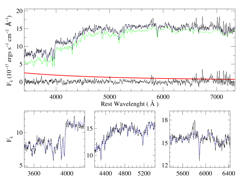
Figure 1: Top panel Spectral synthesis for the BL Lac type object J000157.23-103117.3, performed by STARLIGHT (blue line) using 150 SSP and six power laws to simulate the AGN continuum emission. The observed spectra (top black line), host galaxy model (green line), AGN component (red line) and residuals (bottom black line) are shown. Bottom panel: We show details of the fittings around the absorption features.

3 MEASUREMENTS

3.1 Stellar velocity dispersion

The 179 BL Lac spectra from the original sample have been retrieved from SDSS-DR7 and corrected for Galactic extinction using the maps of Schlegel, Finkenber & Davis (1998). Then they are brought to the rest frame and resampled from 3400 to 9100 Å in steps of 1Å with a flux normalization by the median flux in the 4010-4060 Å  region. We use the stellar population synthesis code STARLIGHT to obtain the best fit to an observed spectrum $O_{\lambda}$ , taking into account the corresponding error $\sigma_{obs}$. The best fit is a combination of single stellar populations (SSP) from the evolutionary synthesis models of Bruzual & Charlot (2003) and power-laws to represent the AGN continuum emission.

The code finds the minimum $\chi^{2}$,

$$\chi^{2}=\sum_{\lambda}\left(\frac{O_{\lambda}-M_{\lambda}}{\sigma_{obs}}\right)$$ (1)

where $M_{\lambda}$ is the model spectrum (SSP and power-laws), obtaining the corresponding physical parameters of the modeled spectrum: Star formation history, $x_{j}$, as a function of a base of SSP models normalized at $\lambda_{0}$, $b_{j,\lambda}$, extinction coefficient of predefined extinction laws, $r_{\lambda}$, and velocity dispersion $\sigma_{\star}$ which obeys the relation:

$$M_{\lambda}=M_{\lambda 0}\left(\sum_{j=1}^{N_{SSP}}x_{j},b_{j,\lambda}r_{\lambda}\right)\otimes G(v_{\star},\sigma_{\star})$$ (2)

In order to model the line-of-sight stellar motions, the code uses a Gaussian distribution of $G$ centered at the velocity $v_{\star}$ with dispersion $\sigma_{\star}$. We use a base of 150 SSPs plus 6 power laws in the form F($\lambda$) = 10²⁰($\lambda$ / 4020)^β, where $\beta$= -0.5, -1, -1.5, -2, -2.5, -3. Each SSP spans six metallicities, Z = 0.005, 0.02, 0.2, 0.4, 1 and 2.5, $Z_{\odot}$, with 25 different ages between 1 Myr and 18 Gyr. Extinction in the galaxy is taken into account in the synthesis, assuming that it arises from a foreground screen with the extinction law of Cardelli et al (1989).

A detailed description of the STARLIGHT code can be found in the publications of the SEAGal collaboration (Cid Fernandes et al. 2005; Mateus et al. 2006; Cid-Fernandes et al. 2007; Asari et al. 2007). We fit all the wavelength range available in the observed spectra (3800-9100 Å) . To estimate the reliable starlight contribution to the optical spectrum we used a uniform weighting to fit all the absorption features within the spectral range mentioned above. When fitting the observed spectrum, we combined a set of power-laws (to account for the AGN continuum luminosity) with stellar populations. This allows the reliable simultaneous decomposition of the host galaxy and AGN optical continuum emission to be performed. However, in the case where the host galaxy is under on-going star formation we should consider the possibility that AGN continuum emission may include a contribution from young stars (Cid-Fernandes et al. 2004).

Table 1 lists the values of the stellar velocity dispersion and AGN continuum luminosity (L₅₁₀₀) for those 78 BL Lacs which were successfully modeled with STARLIGHT. The uncertainties in $\sigma_{\star}$ are the typical errors in the synthesis method, suggested by Cid Fernandes (2005) based on the S/N at 4020 Å . The spectral synthesis result for the BL Lac type object J000157.23-103117.3 is shown in Figure 1, the top-panel shows observed spectra (top black line), host galaxy model (green line), AGN component (red line) and residuals (bottom black line) are shown. In the bottom-panel , we show details of the modeling around the absorption features.

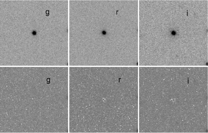
Figure 2: GALFIT decomposition for the BL Lac type object J084225.51+025252.7. We show (top panel) the 2D original images in the $g,r$ and $i$ SDSS-bands, and (bottom panel) residuals after subtracting the galaxy model from the original images.

3.2 Bulge luminosity

We have modelled the surface brightness profiles of the BL Lac host galaxies with the two dimensional image decomposition program GALFIT (Peng et al. 2002). The host galaxy imaging has been retrieved from the SDSS photometry images in $g,r$ and $i$ bands. Previous studies (Falomo et al. 2000, Scarpa et al. 2000, Urry et al. 2000, Nilsson et al. 2003, O’Dowd & Urry 2005 ) have shown that the luminosity profile of BL Lac host galaxies is better represented by an $r^{1/4}$ law (de Vaucouleurs profile). Therefore, we assume a de Vaucouleurs profile to model the host galaxy surface brightness in the sample of 78 BL Lac objects selected as mentioned in the previous section (3.1). The initial guesses of the parameters were obtained using Sextractor (Bertin 1996). Also, we used Sextractor to create mask images for the fitting. We selected bright non-saturated stars in the BL Lacs fields as PSFs. Sky background was fitted first and left fixed during model fitting. In this way, the total number of parameters is reduced when de Vaucouleurs profiles are being computed.

Every BL Lac galaxy is modeled in the g, r and i  SDSS bands, independently. Then, by comparing the quality of the fittings in the 3 bands we decide on the total quality of the fitting. Only the galaxies with good fittings in all three bands are considered as part of our analysis. In Table 1, we list the 71 BL Lac host galaxies best fitted with a simple de Vaucouleurs profile. The bulge magnitude in each band is estimated by using the total magnitude of the galaxy and finally the bulge magnitude in R-band (M_R) has been computed using the photometric transformation equations found by Jester et al. (2005). The final bulge R-band magnitudes have been corrected for Galactic extinction (Schlegel et al. 1998) and we apply the K-correction from Poggianti (1997). We include in Table 1 the absolute bulge magnitudes for our best fits. Figure 2 shows the results of the structural decomposition for the BL Lac object J084225.51+025252.7.

SDSS	Other name	$\sigma_{\star}$	MBH($\sigma_{\star}$)	MR	MBH(MR)	L5GHz	L5100	L1keV	$\nu_{peak}$	Class
(1)	(2)	(3)	(4)	(5)	(6)	(7)	(8)	(9)	(10)	(11)
J000157.23-103117.3	NVSS J000157-103118	286.26$\pm$ 9.47	8.76$\pm$0.10	…	…	31.82	28.32	25.91	13.60	LBL
J005620.07-093629.7	PMN J0056-0936	309.43$\pm$ 4.06	8.89$\pm$0.09	-22.24$\pm$…	8.39$\pm$0.17	31.51	28.55	$<$26.41	16.88	HBL
J020106.17+003400.2	NVSS J020106+003402	208.79$\pm$15.92	8.21$\pm$0.15	-22.48$\pm$0.01	8.51$\pm$0.17	31.60	28.96	$<$27.29	19.85	HBL
J073701.86+284646.0		171.92$\pm$11.56	7.87$\pm$0.13	-21.96$\pm$0.02	8.25$\pm$0.17	31.57	28.89	$<$26.66	17.47	HBL
J075437.07+391047.7		188.47$\pm$10.15	8.03$\pm$0.11	-22.04$\pm$0.01	8.29$\pm$0.17	31.14	28.46	$<$25.40	14.20	LBL
J075846.99+270515.5		198.80$\pm$11.71	8.12$\pm$0.12	-20.46$\pm$0.01	7.50$\pm$0.15	31.29	27.99	25.01	12.12	LBL
J080018.79+164557.1		279.41$\pm$15.16	8.71$\pm$0.12	-22.80$\pm$0.06	8.67$\pm$0.18	32.25	29.10	27.39	17.77	HBL
J080938.88+345537.1	B2 0806+35	261.81$\pm$17.39	8.60$\pm$0.14	-21.47$\pm$…	8.00$\pm$0.16	31.52	28.13	$<$26.22	18.29	HBL
J084225.51+025252.7	NVSS J084225+025251	209.30$\pm$11.83	8.21$\pm$0.12	-22.94$\pm$0.01	8.74$\pm$0.17	32.00	29.28	$<$26.75	16.28	HBL
J085036.20+345522.6	GB6 J0850+3455	244.58$\pm$12.05	8.48$\pm$0.11	-22.44$\pm$0.01	8.49$\pm$0.17	31.31	28.63	$<$25.87	15.39	LBL
J085638.50+014000.6	NVSS J085638+014000	190.96$\pm$22.76	8.05$\pm$0.22	-22.65$\pm$0.26	8.60$\pm$0.22	31.65	29.06	26.53	16.58	HBL
J085749.80+013530.3	PMN J0857+0135	260.24$\pm$ 8.70	8.59$\pm$0.09	-23.24$\pm$0.01	8.89$\pm$0.18	32.32	29.29	$<$26.61	14.50	LBL
J090314.70+405559.8		199.99$\pm$21.12	8.13$\pm$0.19	…	…	31.52	28.31	$<$26.60	17.47	HBL
J090953.28+310603.1		264.78$\pm$ 8.99	8.62$\pm$0.09	-23.19$\pm$0.02	8.87$\pm$0.18	32.24	29.09	$<$27.18	17.40	HBL
J091045.30+254812.8		223.21$\pm$24.20	8.32$\pm$0.20	-22.47$\pm$0.02	8.50$\pm$0.17	32.27	28.80	26.41	13.90	LBL
J091651.94+523828.3		238.27$\pm$11.69	8.44$\pm$0.11	…	…	31.92	28.77	$<$26.82	17.22	HBL
J093037.57+495025.6	NVSS J093037+495026	276.72$\pm$13.08	8.70$\pm$0.11	-21.61$\pm$0.01	8.07$\pm$0.16	31.24	28.81	$<$27.48	21.13	HBL
J094022.44+614826.1	NVSS J094022+614825	228.58$\pm$17.25	8.36$\pm$0.15	-21.95$\pm$0.01	8.25$\pm$0.16	31.10	28.55	$<$26.55	18.96	HBL
J094542.23+575747.7	GB6 J0945+5757	256.76$\pm$11.30	8.57$\pm$0.10	-23.00$\pm$0.01	8.77$\pm$0.18	32.12	29.20	$<$25.65	11.52	LBL
J100444.76+375211.9	87GB 100148.8+380726	236.25$\pm$15.77	8.42$\pm$0.13	-22.98$\pm$0.01	8.76$\pm$0.18	32.44	29.22	$<$26.90	15.09	LBL
J100811.42+470521.4	NVSS J100811+470526	212.18$\pm$11.26	8.23$\pm$0.11	-22.08$\pm$0.02	8.31$\pm$0.17	31.21	28.98	$<$27.70	19.67	HBL
J101706.67+520247.2		240.21$\pm$17.79	8.45$\pm$0.14	-22.37$\pm$0.01	8.45$\pm$0.17	32.26	28.89	$<$26.00	12.41	LBL
J102013.76+625010.1		230.21$\pm$20.52	8.38$\pm$0.17	…	…	31.82	28.60	$<$26.14	14.50	LBL
J102523.04+040229.0	PMN J1025+0402	171.02$\pm$14.44	7.86$\pm$0.16	-21.69$\pm$0.01	8.12$\pm$0.16	31.82	28.49	$<$26.30	15.09	LBL
J103317.94+422236.4	GB6 J1033+4222	245.46$\pm$24.05	8.49$\pm$0.18	-22.03$\pm$0.01	8.28$\pm$0.17	31.67	28.34	$<$25.74	13.60	LBL
J103346.39+370825.1		311.21$\pm$15.68	8.90$\pm$0.12	…	…	31.45	29.06	$<$26.83	18.66	HBL
J104029.01+094754.2		315.35$\pm$11.63	8.93$\pm$0.11	-22.44$\pm$0.01	8.49$\pm$0.17	31.74	28.94	27.17	18.96	HBL
J105606.61+025213.4	NVSS J105606+025227	184.21$\pm$19.86	7.99$\pm$0.20	-21.69$\pm$0.25	8.12$\pm$0.21	30.93	28.59	$<$27.43	22.83	HBL
J110222.94+380122.5		262.50$\pm$21.49	8.60$\pm$0.16	-22.29$\pm$0.02	8.42$\pm$0.17	32.04	28.86	26.22	13.90	LBL
J110356.14+002236.3		249.22$\pm$23.42	8.51$\pm$0.18	-22.42$\pm$0.02	8.48$\pm$0.17	32.08	28.79	25.96	12.71	LBL
J112059.74+014456.9		210.44$\pm$22.18	8.22$\pm$0.19	-22.19$\pm$0.12	8.36$\pm$0.18	32.02	28.71	$<$26.83	16.28	HBL
J114023.48+152809.7		262.01$\pm$13.73	8.60$\pm$0.12	-22.88$\pm$…	8.71$\pm$0.17	32.07	29.21	$<$27.24	17.77	HBL
J114535.10-034001.4		186.99$\pm$19.43	8.01$\pm$0.19	-21.66$\pm$0.03	8.10$\pm$0.16	30.98	28.04	$<$26.81	20.45	HBL
J115404.55-001009.8		209.72$\pm$12.32	8.21$\pm$0.12	-22.17$\pm$0.01	8.35$\pm$0.17	31.30	28.65	$<$26.95	19.55	HBL
J120208.65+444422.4	B3 1159+450	262.82$\pm$ 7.52	8.61$\pm$0.09	-22.75$\pm$0.09	8.65$\pm$0.18	32.18	29.32	25.84	15.92	LBL
J120303.50+603119.1	GB6 J1203+6031	195.69$\pm$12.86	8.09$\pm$0.13	-21.46$\pm$…	8.00$\pm$0.16	31.35	28.92	$<$25.14	12.41	LBL
J120412.11+114555.4		251.26$\pm$19.47	8.53$\pm$0.15	-22.90$\pm$0.10	8.72$\pm$0.18	31.70	29.44	$<$26.76	17.47	HBL
J122300.30+515313.9		187.26$\pm$21.14	8.02$\pm$0.21	-21.81$\pm$0.02	8.18$\pm$0.16	31.16	28.85	26.13	16.88	HBL
J122809.13-022136.1		177.01$\pm$22.48	7.92$\pm$0.23	-21.74$\pm$0.02	8.14$\pm$0.16	30.69	28.39	$<$26.82	21.64	HBL
J123123.90+142124.4	GB6 J1231+1421	312.09$\pm$10.34	8.91$\pm$0.10	-23.00$\pm$…	8.77$\pm$0.18	32.00	29.39	26.48	14.91	LBL
J123623.01+390001.0	GB6 J1236+3859	253.51$\pm$14.53	8.54$\pm$0.12	-23.22$\pm$0.01	8.88$\pm$0.18	32.25	29.23	$<$26.51	16.61	LBL
J123739.08+625842.8		215.18$\pm$11.40	8.26$\pm$0.11	-22.68$\pm$0.02	8.61$\pm$0.17	31.54	29.00	$<$27.06	15.98	HBL
J123831.24+540651.8		264.56$\pm$20.68	8.62$\pm$0.15	-22.17$\pm$0.01	8.36$\pm$0.17	31.70	28.71	25.46	12.41	LBL
J124834.30+512807.8	87GB 124615.8+514411	263.17$\pm$ 8.24	8.61$\pm$0.09	-23.39$\pm$0.01	8.96$\pm$0.18	32.56	29.44	$<$26.38	12.41	LBL
J125347.00+032630.3		218.17$\pm$17.82	8.28$\pm$0.16	-21.81$\pm$0.01	8.18$\pm$0.16	31.02	28.18	$<$25.53	15.09	LBL
J131330.12+020105.9		254.58$\pm$13.41	8.55$\pm$0.11	-22.72$\pm$0.02	8.63$\pm$0.17	32.33	29.06	$<$26.54	14.20	LBL
J132301.00+043951.3		280.33$\pm$20.30	8.72$\pm$0.15	-22.28$\pm$0.01	8.41$\pm$0.17	31.67	28.50	$<$26.90	18.07	HBL
J132617.70+122958.7		269.02$\pm$16.43	8.65$\pm$0.13	-21.95$\pm$0.01	8.24$\pm$0.16	31.59	28.49	$<$26.89	16.32	HBL
J133102.91+565541.8		224.27$\pm$22.19	8.33$\pm$0.18	-21.67$\pm$0.03	8.10$\pm$0.16	30.88	28.46	$<$26.27	18.66	HBL
J133105.70-002221.2		181.24$\pm$19.87	7.96$\pm$0.20	-21.61$\pm$0.01	8.07$\pm$0.16	31.21	28.41	$<$26.00	16.28	HBL
J134105.10+395945.4		258.51$\pm$14.22	8.58$\pm$0.12	-22.18$\pm$0.01	8.36$\pm$0.17	31.59	28.19	$<$26.82	20.06	HBL
J134136.23+551437.9	87GB 133948.0+552941	222.53$\pm$13.45	8.32$\pm$0.12	-21.90$\pm$0.02	8.22$\pm$0.16	31.65	28.65	$<$26.16	15.39	LBL
J134502.30+553914.2		229.72$\pm$20.08	8.37$\pm$0.16	-21.52$\pm$0.01	8.03$\pm$0.16	29.94	28.39	24.96	17.17	HBL
J134633.98+244058.4	NVSS J134634+244100	209.73$\pm$15.24	8.21$\pm$0.14	-22.24$\pm$0.01	8.39$\pm$0.17	31.37	28.34	25.16	12.41	LBL
J135314.08+374113.9	87GB 135107.4+375518	289.96$\pm$18.72	8.78$\pm$0.14	-22.75$\pm$0.26	8.64$\pm$0.22	31.70	28.76	$<$26.13	14.79	LBL
J140121.13+520928.9		227.32$\pm$20.68	8.35$\pm$0.17	-22.69$\pm$0.02	8.61$\pm$0.17	32.07	29.06	$<$26.87	16.28	HBL
J140330.85+360651.1		122.47$\pm$21.26	7.27$\pm$0.32	-21.20$\pm$0.02	7.87$\pm$0.16	30.78	28.50	25.47	15.98	HBL
J140923.50+593940.7		258.21$\pm$17.87	8.58$\pm$0.14	-23.45$\pm$0.01	9.00$\pm$0.18	32.27	29.11	$<$27.26	16.63	HBL
J141030.84+610012.8		300.91$\pm$23.53	8.84$\pm$0.16	-22.47$\pm$0.02	8.50$\pm$0.17	31.40	28.62	$<$27.25	20.25	HBL
J142832.60+424021.0	87GB 142634.5+425353	260.35$\pm$14.53	8.59$\pm$0.12	-22.14$\pm$…	8.34$\pm$0.17	31.35	28.85	$<$27.40	18.55	HBL
J144248.28+120040.2		310.80$\pm$13.44	8.90$\pm$0.11	-22.00$\pm$0.01	8.27$\pm$0.17	31.77	29.02	$<$26.98	16.45	HBL
J145326.52+545322.4		211.80$\pm$22.71	8.23$\pm$0.20	-21.45$\pm$0.01	8.00$\pm$0.16	29.62	28.14	$<$24.78	17.77	HBL
J153447.21+371554.5	87GB 153254.4+372523	154.11$\pm$12.19	7.67$\pm$0.15	-21.48$\pm$0.02	8.01$\pm$0.16	31.15	28.70	$<$25.35	14.26	LBL
J160519.04+542059.9		165.26$\pm$18.65	7.80$\pm$0.21	-21.02$\pm$0.03	7.78$\pm$0.16	30.90	28.30	$<$26.93	21.04	HBL
J161541.21+471111.7		218.22$\pm$13.65	8.28$\pm$0.13	-22.13$\pm$…	8.34$\pm$0.17	32.09	28.81	25.43	10.63	LBL
J161706.32+410647.0		184.60$\pm$ 9.41	7.99$\pm$0.11	-22.55$\pm$0.01	8.54$\pm$0.17	32.16	29.10	$<$26.71	14.41	LBL
J162839.03+252755.9		311.76$\pm$19.34	8.91$\pm$0.14	-22.38$\pm$0.02	8.46$\pm$0.17	31.90	28.72	$<$26.65	16.28	HBL
J163709.50+432600.3	NVSS J163709+432600	299.05$\pm$11.90	8.83$\pm$0.11	-23.09$\pm$0.01	8.81$\pm$0.18	32.29	29.18	$<$25.94	11.82	LBL
J163726.66+454749.0	B3 1635+458	245.11$\pm$23.43	8.49$\pm$0.18	-22.10$\pm$0.01	8.32$\pm$0.17	31.28	28.44	$<$26.11	16.58	HBL
J164419.97+454644.4	B3 1642+458	304.30$\pm$17.31	8.86$\pm$0.13	-22.24$\pm$0.23	8.39$\pm$0.20	32.27	28.72	$<$26.63	14.79	LBL
J165109.19+421253.4		175.21$\pm$18.60	7.90$\pm$0.20	-21.35$\pm$0.01	7.94$\pm$0.16	31.60	28.54	25.60	17.82	LBL
J171427.40+560156.0		268.51$\pm$23.41	8.64$\pm$0.17	…	…	31.53	28.70	$<$26.59	17.47	HBL
J172918.78+525559.2		175.31$\pm$14.80	7.90$\pm$0.16	-22.85$\pm$0.36	8.69$\pm$0.25	31.91	29.08	$<$26.79	16.58	HBL
J211037.75-072412.9	NVSS J211038-072408	254.84$\pm$17.50	8.55$\pm$0.14	-21.79$\pm$0.03	8.17$\pm$0.16	30.59	28.47	25.59	17.17	HBL
J211611.89-062830.4		293.34$\pm$13.26	8.80$\pm$0.11	-22.19$\pm$0.01	8.37$\pm$0.17	31.61	28.93	26.13	15.39	LBL
J221109.88-002327.4		273.75$\pm$24.05	8.68$\pm$0.17	…	…	32.40	28.86	26.70	14.50	LBL
J222944.18-003426.6		260.27$\pm$12.75	8.59$\pm$0.11	-22.90$\pm$0.05	8.72$\pm$0.18	30.93	28.65	26.82	20.74	HBL
J235604.01-002353.7		182.99$\pm$20.81	7.97$\pm$0.21	-21.83$\pm$0.01	8.19$\pm$0.16	31.12	28.68	$<$26.20	17.47	HBL

Table 1: Column description: (1) SDSS name, (2) alias given by radio surveys, (3) stellar velocity dispersions in units (km s^-1), (4) log of black hole mass estimated from stellar velocity dispersion in units of (M_⊙), (5) R-band bulge absolute magnitude, (6) log of black hole mass estimated from R-band bulge luminosity in units of (M_⊙), (7) log of radio luminosity at 5GHz, (8) log of nuclear optical continuum luminosity at 5100 Å , (9) log of X-ray luminosity at 1 keV, (10) log of synchrotron peak frequency in (Hz) and (11) the classification of BL Lacs based on the X-ray to radio flux ratio, following Padovani & Giommi (1995). Note: All luminosities in this table are in units of erg s^-1 Hz^-1 and synchrotron peak frequencies in italic font have been taken from Nieppola et al. (2006)

4 BLACK HOLE MASSES

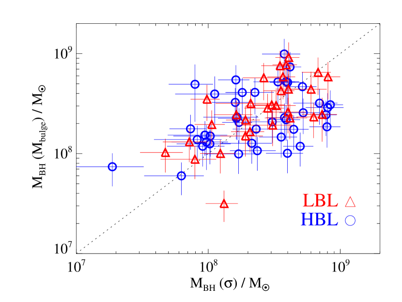
Figure 3: Comparison of black hole mass estimates of 71 BL Lac type objects from the stellar velocity dispersion and from the R-band bulge magnitude. There is no significant difference in the black hole mass range between LBL (open-triangles) and HBL (open-circles) objects. The dashed line respresents the one-to-one correspondence.

Following Tremaine et al. (2002) and McLure and Dunlop (2002), the expressions to estimate black hole masses can be expressed in the following forms:

$$\log M_{BH}(\sigma_{\star})=4.02(\pm 0.32)\log\left(\frac{\sigma_{\star}}{\sigma_{0}}\right)+8.13(\pm 0.06)$$ (3)

$$\log M_{BH}(M_{R})=-0.50(\pm 0.02)~{}M_{R}+2.73(\pm 0.48)$$ (4)

where $\sigma_{\star}$ is the stellar velocity dispersion, $\sigma_{0}=$ 200 km s^-1 and M_R is the absolute bulge magnitude in R band (corrected to our adopted cosmology). The black hole masses derived from $\sigma_{\star}$ and M_R are designated as M${}_{BH}(\sigma_{\star})$ and M${}_{BH}(M_{R})$, respectively in columns 4 and 6 of Table 1. As can be seen from Figure 3, there is a generally good agreement between black hole masses estimated by both methods. The average values derived from $\sigma_{\star}$ and $M_{R}$ are $\langle log~{}M_{BH}\rangle_{\sigma_{\star}}=8.38\pm 0.04$ and $\langle log~{}M_{BH}\rangle_{M_{R}}=8.38\pm 0.03$, respectively, with an average difference of $\langle\Delta log~{}M_{BH}\rangle=-0.008\pm 0.038$ . This result gives us additional confidence in the reliability of our black hole mass estimations. Since the relation M${}_{BH}-\sigma_{\star}$ suffers of less intrinsic dispersion, is the most accurate (Vestergaard 2009) and $\sigma_{\star}$ measurements are not affected by potential beaming effects, in the following we focus our analysis on black hole masses estimated via stellar velocity dispersion.

Figure 4 shows the distribution of black hole masses estimated for HBL and LBL objects. As can be seen, the ranges of black hole mass in both populations are consistent with each other. The Kolmogorov-Smirnov test shows that there is no a significant difference between the distributions of black hole mass for HBL and LBL objects, confirming results in previous BL Lacs studies(Falomo et al. 2002; 2003, Woo et al. 2005)

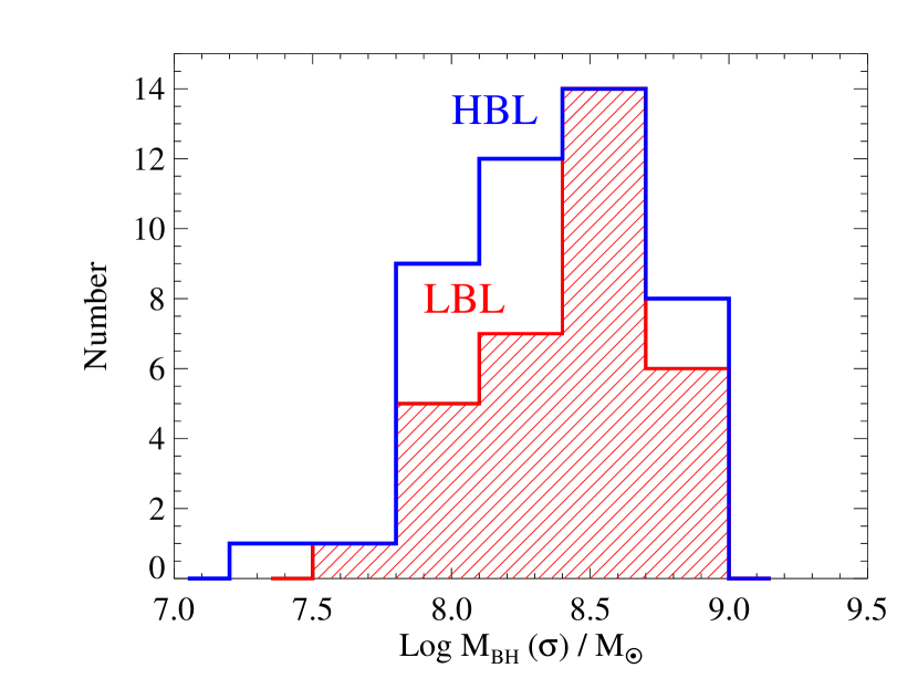
Figure 4: M_BH distribution for 78 BL Lac type objects. There is no a significant difference in the black hole mass distribution between HBL (blue) and LBL (red) objects.

5 THE BLACK HOLE MASS- LUMINOSITY RELATIONSHIP

Figure 5: Correlation between black hole mass and luminosity at $5GHz$ (top panel), $5100\AA~{}$ (middle panel) and $1keV$ (bottom panel). HBL and LBL are shown by open circles and open triangles, respectively. The solid line gives the ordinary least-squares fit to the data, whereas fitted relations for LBL and HBL separately are shown as dotted and dashed lines, respectively. See Table 2 for the correlation and best-fit parameters.

In Figure 5 we plot our black hole mass estimations versus multiwavelength luminosities. Luminosities at 5 GHz and 1keV have been taken from Plotkin et al. (2008). Disentangling the AGN component from the host galaxy contribution as described in section 3.1 allowed us to recover the optical nuclear continuum luminosity at 5100 Å. The solid green lines in the panels of Figure 5 represent our fit to the data. Treating M_BH as the independent variable, an ordinary least-squares fit yields

$$L_{5GHz}\propto M_{BH}^{\ 0.63\pm 0.16}$$ (5)

$$L_{5100\AA}\propto M_{BH}^{\ 0.30\pm 0.11}$$ (6)

$$L_{1keV}\propto M_{BH}^{\ 0.48\pm 0.21}$$ (7)

The Spearman rank correlation coefficients listed in Table 2, confirm a positive correlation for the above relations at high significance level. These relations are fits for the combined HBL and LBL populations. However, the best-fit parameters and correlation strengths are slightly changed when HBLs and LBLs are considered separately. The fitted relations for LBL and HBL are shown in Figure 5 as dotted and dashed lines, respectively. Table 3 lists the best-fit parameters for each BL Lac population. It is worth noticing that the slopes derived for the LBL population are somewhat steeper than those derived for the HBL population.

The correlation between black hole mass and X-ray luminosity becomes stronger and more significant when computed separately for LBL and HBL populations (see Table 2). This arises naturally if we bear in mind that HBL and LBL are by definition two different populations in the X-ray regime. The Spearman rank correlation test provides evidence of a positive correlation between M_BH and L_5GHz, L₅₁₀₀ and L_1keV at a confidence level $>98\%$ when restricted only to LBL. We note that when considering exclusively HBLs, the correlations between M_BH and L_5GHz, L_1keV are weaker, though still significant ($>95\%$). However, the Spearman rank correlation test between black hole mass and optical luminosity for HBL provides only evidence of a trend (at 80$\%$ confidence), this may betray the presence of a stellar contribution in the optical continuum luminosity of HBLs. Whether the stellar component differs significantly between LBL and HBL will be addressed in a forthcoming paper. As mentioned before, the correlations described above have been computed using the black hole mass derived from stellar velocity dispersion. However, the best-fit parameters are virtually unchanged when the estimations of black hole mass via bulge magnitude are considered.

Table 2: Spearmank’s correlation coefficients between black hole mass and multiwavelength luminosities for BLLacs in our sample. Partial correlation methods have been performed for correlations of the luminosity-luminosity type, in order to remove the common dependence with redshift. We consider a correlation to be significant if the probability that the correlation is given by chance is $P\leq 5\times 10^{-2}$ or in other words at a significance level of 95%

		All			LBL			HBL
A1	A2	$\rho$	$P$		$\rho$	$P$		$\rho$	$P$
$M_{\rm BH}$	$L_{\rm 5GHz}$	0.4	2$\times 10^{-4}$		0.5	5$\times 10^{-3}$		0.4	1$\times 10^{-2}$
$M_{\rm BH}$	$L_{\rm 5100\AA}$	0.3	9$\times 10^{-3}$		0.5	8$\times 10^{-3}$		0.2	2$\times 10^{-1}$
$M_{\rm BH}$	$L_{\rm 1keV}$	0.2	7$\times 10^{-2}$		0.4	2$\times 10^{-2}$		0.3	4$\times 10^{-2}$
$L_{\rm 5GHz}$	$L_{\rm 5100\AA}$	0.6	3$\times 10^{-9}$		0.5	6$\times 10^{-3}$		0.7	2$\times 10^{-8}$
$L_{\rm 5GHz}$	$L_{\rm 1keV}$	0.1	7$\times 10^{-1}$		0.4	1$\times 10^{-2}$		0.4	8$\times 10^{-3}$

Table 3: Best fit parameters for the M_BH-luminosity and luminosity-luminosity relations shown in Figure 5 and 6, respectively.

	All	LBL	HBL
	$x$	$x$	$x$
$L_{\rm 5GHz}\propto M_{\rm BH}^{x}$	$0.63\pm 0.16$	$0.70\pm 0.21$	$0.51\pm 0.19$
$L_{\rm 5100\AA}\propto M_{\rm BH}^{x}$	$0.30\pm 0.11$	$0.48\pm 0.19$	$0.18\pm 0.14$
$L_{\rm 1keV}\propto M_{\rm BH}^{x}$	$0.48\pm 0.22$	$0.71\pm 0.26$	$0.48\pm 0.21$
$L_{\rm 5GHz}\propto L_{\rm 5100}^{x}$	$1.00\pm 0.13$	$0.86\pm 0.14$	$1.02\pm 0.18$
$L_{\rm 5GHz}\propto L_{\rm 1keV}^{x}$	$0.24\pm 0.09$	$0.63\pm 0.10$	$0.60\pm 0.10$

In search of some physical insight into the black hole mass - luminosity relation, we explore correlations between X-ray/optical and radio emission. For luminosity-luminosity correlations we have taken into account the common dependence with the redshift by using partial correlation analysis. The results of our partial correlation analysis between luminosities are given in Table 2. Radio and optical continuum luminosities are shown in the top panel of figure 6, where a significant correlation between L_5GHz and L₅₁₀₀ is found at very high confidence level with a correlation coefficient $\rho=0.6$ and the probability that such correlation is not due to chance is $>99.9\%)$ . This suggests that the emission in the two bands has a similar origin, more specifically non-thermal radiation from the jets. The best fit to the combined sample is shown as a solid line in the top panel of Figure 6, whereas dotted and dashed lines represent the best fits for the LBL and HBL populations.

Nevertheless, when attempting to compare the distributions of L_5GHz and X-ray luminosities, it turns out that we do not find evidence of significant correlation when the dependence of redshift is removed (see bottom panel in Figure 6). However, when HBL and LBL are considered separately, the Spearman rank correlation strength between luminosities becomes higher and significant ($>98\%$). This comes naturally, considering that HBL and LBL form two different populations in the X-ray regime. Table 1 lists correlation and best-fit parameters for each population. We stress that when computing correlations with the X-ray luminosities, we use upper limits for those sources non detected in Xrays. It is conceivable that real values would produce an even higher separation between HBL and LBL populations, which would not change the significance of correlations computed.

Figure 6: Correlation between radio luminosity at 5GHz and optical continuum (left panel) and Xray (right panel) emission.The correlation between X-rays and radio emission only holds when considering HBL and LBL populations separately. The solid line gives the ordinary least squares fit to the data, where fitted relations for LBL and HBL populations are shown as dotted and dashed lines, respectively. Best-fit parameters and correlation coefficients among luminosities are listed in Table 3.

6 Discussion

In this work we have measured stellar velocity dispersions and bulge luminosities for BL Lac objects identified in the SDSS and FIRST surveys, enabling us to estimate masses for the black holes in our sample. The range of black hole masses computed from stellar velocity dispersion is in substantial agreement with those estimated from R-band bulge magnitude, the average difference of black hole masses estimated by both methods is $\langle\Delta log~{}M_{BH}\rangle=-0.008\pm 0.038$ . Within the sample of BL Lacs considered, LBL and HBL sources are indistinguishable in terms of black hole mass.

We found that in our sample of BL Lacs, the black hole mass correlates at high significance level with radio (5GHz), optical nuclear (5100 Å), and X-ray (1keV) luminosities. Radio luminosity at 5GHz correlates tightly with the nuclear optical luminosity and with X-ray luminosity when correlation coefficients are computed for LBL and HBL, separately, implying that the emission in the optical and X-ray bands share a similar origin, more specifically non-thermal emission from the jets.

We note that the strong correlation between black hole mass and radio luminosity found in this study is in disagreement with the results of Woo et al (2005,) who found no evidence of such a correlation using a sample of BL Lacs. The range of black hole masses found in this work are similar than those found in Woo et al. (2005) and other previous works (Falomo et al. 2003; Dunlop et al. 2003). Then, these apparently conflicting results may be attributable to the literature compilation done by Woo et al. (2005) where the measurements have not been obtained in a homogeneous way. Whereas in this work all the black hole masses have been estimated in a uniform fashion, data taken with the same instruments. Besides, various studies have found a roughly linear correlation between black hole mass and radio luminosities (e.g. Falomo et al. 2003, Dunlop et al. 2003, Arshakian et al. 2005), although consistent with our study they report a slope higher than ours. This apparent disagreement may be related to the mixed population of radio sources involved in those studies and also due to the different luminosity coverage. The black hole masses used in the previous studies are compiled from literature and mainly computed from the broad emission lines, which might introduce potential uncertainties regarding the location, geometry and non-virialization effects in the BLR (Arshakian et al. 2010, León-Tavares et al. 2010, Ilić et al. 2009). The advantage of this work over the previous ones, is that our measurements have been performed in a uniform fashion and the 78 black hole masses estimated from the stellar velocity dispersion are free of the potential uncertainties mentioned above.

Figure 7: The distribution of radio-X-ray spectral index ($\alpha_{rx}$) and synchrotron peak frequency ($\nu_{peak}$) for BLLacs which SED has been succesfully modelled in Nieppola et al. 2006. The dashed line gives the ordinary least squares fit to the data.

Since it is well established that the synchrotron emission in BLLacs (and in blazars in general) is affected by relativistic beaming effects due to a fast jet aligned close to our line of sight (Blandford & Konigl 1979), then we must expect the emission in BL Lacs to be Doppler boosted. However, we should be aware that luminosities in BLLacs might not exclusively depend on Doppler boosting effects but on intrinsic physics conditions.

As a consequence, the correlation M${}_{BH}-luminosity$ found in this work, might be understood either as an evidence of observed dependence between black hole mass and Doppler boosting effects (Arshakian et al. 2005, Valtaoja et al. 2008, Torrealba et al. 2008) or as a relationship between black hole mass and intrinsic physics conditions in each source (i.e. magnetic field strength, jet composition, etc). Unfortunately we can not test in situ the correlation between black hole mass and Doppler factor with our sample of BL Lacs, due to the fact that computation of variability Doppler factors are observationally expensive, requiring long-term monitoring. However, we may attempt to disentangle the population of BLLacs for which luminosity is most likely Doppler boosted, as follows.

Figure 8: Black-hole mass - synchrotron peak frequency plane, where the color scale corresponds to the intensity of radio emission, darker colors corresponding to brightest radio-jets . The region located at the bottom-right of the plane is exclusively populated by the heaviest black-holes ($M_{BH}>10^{8.25}$), brightest radio-jets ($L_{5GHz}>10^{31.5}$) and the lowest synchrotron peak frequencies ($\nu_{peak}<10^{16}$). Sources contained in this beamed-region fullfill the criteria for which broad band emission is dominated by Doppler boosting effects.

Starting from the hypothesis that emission strength in BL Lacs depends primarily on Doppler boosting effects which are characterized by the Doppler factor ($D$), then derived expressions (5-7) can be seen as L$(D)\propto M_{BH}$. Furthermore, it is well established that emission from the relativistic beamed jet is responsible for the lower energy-peak in the BL Lacs SED and its position on the log$\nu$-axis is defined as the synchrotron-peak frequency ($\nu_{peak}$). Using a sample of 89 blazars, Nieppola et al. (2008) found an inverse dependence between the Doppler boosting factors and peak frequencies ($D\propto\nu_{peak}^{-1}$). Such a relation holds for $\nu_{peak}<10^{16}$ (Hz), above which Nieppola et al. (2008) argued the D$\sim 1$. Based on this, we may assume that Doppler boosted emission follow the relation L$(D)\propto\nu_{peak}^{-1}$. According to these expressions, we should expect the dependence between black-hole mass and synchrotron peak frequency to be inversely proportionally (M${}_{BH}\propto\nu_{peak}^{-1}$) for BL Lacs where emission is dominated by Doppler boosting effects.

In order to find whether BLLacs in our sample fulfill the relations mentioned above, we compile synchrotron peak frequencies estimates for our sample. SEDs for 18 BLLacs contained in this study have been constructed and successfully modeled in Nieppola et al. (2006). The distribution of peak frequencies with their respective broad band spectral indexes ($\alpha_{RX}$) is shown in Figure 7. Information about the broad band spectral indexes has been taken from Table 6 in Plotkin et al. (2008) . A common least-square fit to the data yields,

$$\alpha_{RX}=(1.23\pm 0.04)+log(\nu_{peak})\times(-0.03\pm 0.01)$$ (8)

This expression allows us to compute the peak frequencies for the rest of our sample. The compiled and computed synchrotron peak frequencies are listed in Table 1. Figure 8 shows the $M_{BH}-\nu_{peak}$ plane where the color scale corresponds to the radio luminosity, darker colors corresponding to brightest radio jets. We note that there is very well defined region located at the bottom-right part of the plane. This region is exclusively populated by the heaviest black-holes($M_{BH}>10^{8.25}$), brightest radio-jets ($L_{5GHz}>10^{31.5}$) and the lowest peak frequencies ($\nu_{peak}<10^{16}$) and in the following we refer to it as the beamed region. 32 out of 78 ($40\%$) BL Lacs in our sample (mostly classified as LBL) are enclosed in this beamed region, fullfilling the criteria for which the broad-band emission is dominated by Doppler boosting effects.

Doppler boosting effects in a relativistic jet are often characterized by the Doppler factor, which is a function of the jet viewing angle and jet speed. Since the jet viewing angle does not play a major role in determining the SED shape in BL Lac type objects (Padovani & Giommi 1995), we may assume that in our entire sample of BLLacs (LBL and HBL), the Doppler boosted luminosities will not strongly depend on the orientation angle but mainly on the speed of the jet. Hence, the correlation $M_{BH}-luminosity$ for BL Lacs inside the beamed region might be understood as a correspondence between M_BH and Doppler factor, being the latest mainly dependent on the speed of the jet. This can be taken as an evidence that more massive black holes produce faster jets in some BL Lac type objects. Thus BLLacs outside the beamed region must have slower jet speeds.

Figure 9 shows the M_BH-L_5GHz plane where the color-scale corresponds to the synchrotron peak frequency. A dashed line has been drawn to approximately separate Doppler boosting dominated BL Lacs, based on their synchrotron peak frecuency ($\nu_{peak}\approx 10^{16}$ Hz). As it can be seen, the separation line coincides with an apparent dichotomy in radio luminosity, most likely influenced by Doppler boosting effects. This implies that all sources above the line would shift downwards in Figure 9 if their intrinsic jet luminosity could be observed. For BL Lacs below the dashed line, Doppler boosting should not be a major factor and the observed correlation between black hole mass and luminosity is likely to be intrinsic. If we consider only sources with $\nu_{peak}>10^{16}$, we are still finding that black hole mass correlates ($\rho=0.3,P=97\%$) with the radio luminosity, roughly of the form M${}_{BH}\propto L_{5GHz}^{0.5}$. The fact that this slope is shallower than that found for BL Lacs with $\nu_{peak}<10^{16}$ (M${}_{BH}\propto L_{5GHz}^{0.8}$) is merely a consequence of Doppler boosting effects on the M${}_{BH}-luminosity$ relation. This suggests an additional intrinsic dependence between black hole mass and luminosity for sources in which luminosity is not Doppler boosting dominated. Whether host-galaxy properties are somewhat responsible for the intrinsic luminosity may be gleaned from the stellar-population synthesis that comes as a byproduct of this study.

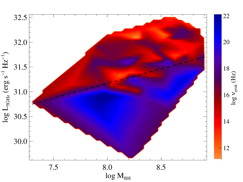
Figure 9: Black-hole mass - radio luminosity plane, where the color scale corresponds to the synchrotron peak frequency. The dashed line is drawn at $\nu_{peak}\approx 10^{16}$ Hz, aiming to divide Doppler boosting dominated BL Lacs (above the line) from sources where Doppler boosting should not be a major factor (below the line) in their luminosity. The correlation between M_BH-L_5GHz is present for the overall sample of BLLacs.

7 SUMMARY

This work presents black hole mass estimations for a sample of 78 BL Lac type objects drawn from the SDSS-FIRST sample of Plotkin et al. (2008). The main findings of this work are as follows:

• Within the sample of BL Lacs considered, HBL and LBL are indistinguishable in terms of black hole mass.

• The black hole mass correlates at high significance level with radio luminosity at 5GHz, optical continuum luminosity at 5100 Å and X-ray luminosity (see Figure 5).

• Furthermore, as it can be seen in Figure 6, optical continuum and X-ray emission are strongly correlated to the radio luminosity, implying that emission in optical and X-ray bands can be associated to relativistic jets.

• When radio luminosity is taken as a third dimension in the plane $M_{BH}-\nu_{peak}$, the sample of BL Lacs separates quite clearly in regions where luminosity is dominated by intrinsic processes and by Doppler beaming effects. The former region is exclusively populated by BL Lacs with the heaviest black holes, lowest synchrotron peak frequencies and brightest jets.

• We have found that for a sizeable fraction (40%) of BLLacs in our sample, the emission is dominated by relativistic beaming effects. For these sources, the correlation between black hole mass and luminosity can be understood as an evidence of a correspondence between black hole mass and Doppler boosting factors.

• If we assume a typical orientation angle for the population of BL Lacs, thus the Doppler boosted emission will not strongly depend on the viewing angle but mainly on the speed of the jet. Therefore, the correlation between the black hole mass and Doppler factor suggested by the results found in this work may imply that more massive black holes produce faster jets.

• For sources which are not Doppler boosted we still find a correlation between black hole mass and radio luminosity, suggesting that it must be intrinsic and more massive black holes produce more luminous jets.

Hopefully, results presented in this work will provide the impetus for more observations that look for such correlation among blazars.

We thank the referee for providing useful comments and suggestions which improved this manuscript. J. Leon-Tavares acknowledges support from the Aalto University postdoctoral program offered by the School of Science and Technology. This work was supported by CONACYT research grant 54480 (México). J. Leon-Tavares would like to thank J.P Torres-Papaqui for his valuable assitance with STARLIGHT. C. Añorve acknowledges support from the CONACYT program for PhD studies. The STARLIGHT project is supported by the Brazilian agencies CNPq, CAPES and FAPESP and by the France-Brazil CAPES/Cofecub program. Funding for the SDSS and SDSS-II has been provided by the Alfred P. Sloan Foundation, the Participating Institutions, the National Science Foundation, the U.S. Department of Energy, the National Aeronautics and Space Administration, the Japanese Monbukagakusho, the Max Planck Society, and the Higher Education Funding Council for England. The SDSS Web Site is http://www.sdss.org/.

The SDSS is managed by the Astrophysical Research Consortium for the Participating Institutions. The Participating Institutions are the American Museum of Natural History, Astrophysical Institute Potsdam, University of Basel, University of Cambridge, Case Western Reserve University, University of Chicago, Drexel University, Fermilab, the Institute for Advanced Study, the Japan Participation Group, Johns Hopkins University, the Joint Institute for Nuclear Astrophysics, the Kavli Institute for Particle Astrophysics and Cosmology, the Korean Scientist Group, the Chinese Academy of Sciences (LAMOST), Los Alamos National Laboratory, the Max-Planck-Institute for Astronomy (MPIA), the Max-Planck-Institute for Astrophysics (MPA), New Mexico State University, Ohio State University, University of Pittsburgh, University of Portsmouth, Princeton University, the United States Naval Observatory, and the University of Washington.

References

- Abdo et al. (2010) Abdo, A. A. et al. 2010, ApJ submitted, (arXiv:1002.0150)
- Arshakian et al. (2005) Arshakian,T. G., Chavushyan, V. H., Ros, E., Kadler M. & Zensus, J. A. 2005, MmSAI, 76, 35
- Arshakian et al. (2010) Arshakian, T. G., León-Tavares, J., Lobanov, A. P., Chavushyan, V. H., Shapovalova, A. I., Burenkov, A. N. & Zensus, J. A. 2010, MNRAS, 401, 1231
- Asari et al. (2007) Asari, N. V., Cid Fernandes, R., Stasińska, G., Torres-Papaqui, J. P., Mateus, A., Sodré, L., Schoenell, W., Gomes, J. M. . 2007, MNRAS, 381, 263
- Blandford & Konigl (1979) Blandford, R. D., & Konigl, A. 1979, ApJ, 232, 34
- Bertin & Arnouts (1996) Bertin, E & Arnouts, S. 1996, A&AS, 117, 393
- Bruzual, G & Charlot (2003) Bruzual, G & Charlot, M. J. 2003, MNRAS, 344, 1000
- Cardelli et al. (1989) Cardelli J. A., Clayton, G. C. & Mathis, J. S. 1989, ApJ, 345, 245
- Cid Fernandes et al. (2004) Cid Fernandes, R., Gu, Q., Melnick, J., Terlevich, E., Terlevich, R., Kunth, D., Rodrigues Lacerda, R., & Joguet, B. 2004, MNRAS, 355, 273
- Cid Fernandes et al. (2005) Cid Fernandes, R., Mateus, A., Sodré, L., Stasińska, G., & Gomes, J. M. 2005, MNRAS, 358, 363
- Cid Fernandes et al. (2007) Cid Fernandes, R., Asari, N. V., Sodré, L., Stasińska, G., Mateus, A., Torres-Papaqui, J. P., & Schoenell, W. 2007, MNRAS, 375, L16
- Dunlop et al. (2003) Dunlop, J. S., McLure, R. J., Kukula, M. J., Baum, S. A., O’Dea, C. P. & Hughes, D. H. 2003, MNRAS, 340, 1095
- Falomo et al. (2000) Falomo, R., Scarpa, R., Treves, A. & Urry, C. M. 2000, ApJ, 542, 731
- Falomo et al. (2002) Falomo, R., Kotilainen, J. K., Treves, A. 2002, ApJL,596, 35
- Falomo et al. (2003) Falomo, R., Kotilainen, J. K., Carangelo, N. & Treves, A. 2003, ApJ, 595, 624
- Ferrarese et al. (2001) Ferrarese, L., Pogge, R. W., Peterson, B. M., Merritt, D., Wandel, A., Joseph, C. L. 2001, ApJL, 555, 79
- Ilić et al. (2008) Ilić, D., Popović, L. Č., León-Tavares, J., Lobanov, A. P., Shapovalova, A. I., Chavushyan, V. H. 2008, MmSAI, 79,1105
- Jester et al. (2005) Jester, S. et al. 2005 ,AJ, 130, 873
- Kaspi et al. (2000) Kaspi, S., Smith, P. S., Netzer, H., Maoz, D., Jannuzi, B. T. & Giveon, U. 2000 ApJ, 533, 631
- Komatsu et al. (2009) Komatsu, E., et al. 2009, ApJS, 180, 330
- León-Tavares et al. (2010) León-Tavares, J., Lobanov, A. P., Chavushyan, V. H., Arshakian, T. G., Doroshenko, V. T. et al. 2010, ApJ, 715, 355
- Lister et al. (2009) Lister, M. L., Cohen, M. H., Homan, D. C., Kadler, M., Kellermann, K. I., Kovalev, Y. Y., Ros, E., Savolainen, T. & Zensus, J. A. 2009, ApJL, 696, 22
- McLure & Dunlop (2002) McLure, R. J. & Dunlop, J. S. , MNRAS, 331, 795
- Mateus et al. (2006) Mateus, A., Sodre, L., Cid Fernandes, R., Stasinska, G., Schoenell, W., & Gomes, J. M. 2006, MNRAS, 370, 721
- Nieppola et al. (2006) Nieppola, E., Tornikoski, M. & Valtaoja, E. 2006, A&A,445, 441
- Nieppola et al. (2008) Nieppola, E., Valtaoja, E., Tornikoski, M., Hovatta, T. & Kotiranta, M. 2008 , A&A, 488, 867
- Nilsson et al. (2003) Nilsson, K., Pursimo, T., Heidt, J., Takalo, L. O., Sillanpää, A., & Brinkmann, W. 2003 A&A, 400, 95
- O’Dowd & Urry (2005) O’Dowd, M. & Urry, C. M. 2005, ApJ, 627, 97
- Padovani & Giommi (1995) Padovani, P., Giommi, P. 1995, ApJ, 444, 567
- Peng et al. (2002) Peng, C. Y., Ho, L. C., Impey, C. D. & Rix, H. 2002, AJ, 124, 266
- Perlman et al. (1996) Perlman, E. S., Stocke, J. T., Wang, Q. D. & Morris, S. L., 1996, ApJ, 456, 451
- Peterson et al. (2004) Peterson, B. M., Ferrarese, L., Gilbert, K. M., Kaspi, S., Malkan, M. A., et al. 2004, ApJ, 613, 682
- Plotkin et al. (2008) Plotkin, R. M., Anderson, S. F., Hall, P. B., Margon, B., Voges, W., Schneider, D. P., Stinson, G., York, D. G. 2008, AJ, 135, 2453
- Poggianti (1997) Poggianti, B. 1997 A&AS, 122, 399
- Savolainen et al. (2010) Savolainen, T., Homan, D. C., Hovatta, T., Kadler, M., Kovalev, Y. Y.; Lister et al. 2010, A& A, 512, 24
- Scarpa et al. (2000) Scarpa, R., Urry, C. M., Padovani, P., Calzetti, D. & OD́owd, M. 2000, ApJ, 532, 740
- Schlegel et al. (1998) Schlegel, D.J., Finkbeiner D.P., & Davis M. 1998, ApJ, 500, 525
- Tremaine et al. (2002) Tremaine, S. et al. 2002, AJ, 574, 740
- Tornikoski et al. (2010) Tornikoski, M., Nieppola, E., Valtaoja, E., León-Tavares, J. & Lähteenmäki, A. 2010, Proceedings of the Workshop ”Fermi meets Jansky - AGN in Radio and Gamma-Rays”, Savolainen, T., Ros, E., Porcas, R.W. & Zensus, J.A. (eds.), MPIfR, Bonn, June 21-23 2010
- Torrealba et al. (2008) Torrealba, J., Chavushyan, V. H., Arshakian, T. G., Cruz-González, I., Ros, E., Zensus, J. A., Bertone, E., Rosa-González, D. 2008, The Nuclear Region, Host Galaxy and Environment of Active Galaxies (Eds. Erika Benítez, Irene Cruz-González, & Yair Krongold) Revista Mexicana de Astronomí a y Astrofísica (Serie de Conferencias) Vol. 32, pp. 48-48
- Urry et al. (2000) Urry, C. M., Scarpa, R., O’Dowd, M., Falomo, R., Pesce, J. E., Treves, A. 2000, ApJ, 532, 816
- Valtaoja et al. (2008) Valtaoja, E., Lindfors, E., Saloranta, P.-M., Hovatta, T., Lähteenmäki, A., Nieppola, E., Torniainen, I. & Tornikoski, M. 2008, ASPC, 386, 388
- Vestergaard (2009) Vestergaard M., 2009, Spring Symposium on “Black Holes” (Cambridge University Press) in press, (astro–ph/0904.2615)
- Woo et al. (2005) Woo, J.-H., Urry, C. M., Van der Marel, R. P., Lira, P., & Maza, J. 2005, ApJ, 631, 762