Extracting resonance parameters from lattice data

Abstract:

Monte Carlo simulations of the 4d O(4) model in the broken phase are performed to determine the parameters of a resonance. The standard method for extracting them on the lattice is through Lüscher’s formula; recently a new method, based on the probability distribution concept, has been proposed. We study the application of these methods and compare them with Monte Carlo data.

1 Introduction

In Quantum Chromodynamics, the current theory of the strong force, many states do not appear directly in scattering experiments, but only indirectly in the behaviour of the scattering cross sections of observable particles. This is because these states, known as resonances, are unstable and decay in a very short time relative to the scattering experiment. Extracting the decay widths and masses of these states is thus an important theoretical challenge.

Lattice Field Theory provides a possible way of extracting these resonance parameters in a non-perturbative fashion. The typical method for extracting particle masses in lattice field theory is to study the decay of a correlator with the same quantum numbers as the particle in question. The large-time behaviour of the correlator is then

$$\lim_{t\rightarrow\infty}C(t)=Ze^{-mt}\ ,$$ (1)

where $m$ is the mass of the lightest particle with the chosen quantum numbers, which can be extracted by fitting the correlator. This method however will not work for resonances. By virtue of being unstable, resonances are above the multiparticle threshold in their channel and never dominate the behaviour of the correlator in a simple manner. Fundamentally resonances are not energy eigenstates of the Hamiltonian, but rather poles of the S-matrix and so are a truly dynamical phenomena.

Given their relation to dynamical scattering processes, resonance parameters can be found using the scattering phase shift $\delta(p)$. The difficulty lies in obtaining information about $\delta(p)$ on a Euclidean lattice. In Ref [1] it was discovered that there is a connection between the behaviour of the two particle energy spectrum in finite volume and the scattering phase shift $\delta(p)$. Hence provided one can accurately determine the energy spectrum it should be possible to obtain $\delta(p)$ and through it the resonance parameters. Recently another method has been proposed in Ref [2]. This method takes the intuition gained from Lüscher’s method to construct a probability distribution which measures the relative frequency of energy levels in the interacting case (resonance present) and the noninteracting case (no resonance); we will refer to this method as the histogram method. It can be shown that the parameters of this probability distribution are fundamentally related to the parameters of the resonance. Furthermore, the method provides a visual tool. The resonance should manifest itself as a peak in the distribution.

Our first discussion on this topic, with an historical introduction and a basic theoretical background, can be found in Ref [3]. In this work we aim to compare and contrast these two methods. In particular we analyse how accurately resonance parameters can be extracted using both methods and also the ambiguity in applying the two methods. A first attempt to test the histogram method on a simple one dimensional model can be found in Ref [4].

2 Theoretical background

2.1 Two particles in a box

In the continuum, two identical non-interacting bosons of mass $m_{\pi}$ characterised by a relative momentum $\vec{p}$, in a box of volume $V=\prod_{i=1}^{3}L_{i}$, have a total energy $E$ given by

$$E=2\sqrt{m_{\pi}^{2}+\vec{p}^{2}}\ ;$$ (2)

where due to the finite volume, the momenta $p_{i}$ are given by $p_{i}=\frac{2\pi}{L_{i}}n_{i}$ with $n_{i}\in Z$. On the lattice the space-time discretization can have a strong effect (see Figure 1) in particular when the volume is small (large momentum) and $m_{\pi}$ is big. The correct expression for the simplest discretisation of the free scalar field is

$$E=4\sinh^{-1}\left[{\frac{1}{2}\sqrt{m_{\pi}^{2}+\tilde{p}^{2}}}\right]\ ,$$ (3)

where $\tilde{p}_{i}=2\sin{\frac{\pi}{L_{i}}n_{i}}$. It is also valuable to use this expression to describe the energy of interacting particles as we will show.

\psfrag{LL}{$L$}\psfrag{EE}{$E_{n}$}\psfrag{MM}{$m_{\pi}=0.46$}\includegraphics[width=156.10345pt,angle={-90}]{figure/noninteractspectr/latt/spectrum.ps}

Figure 1: The total energy $E$ for four different levels in the continuum (black lines) and in the lattice (red lines) case versus $L$.

In a general case such as QCD, where an expression like Eq. 3 is not available, we need to determine the non-zero-momentum single-particle energy levels numerically and then, to determine the two-particle energy spectrum, simply multiply the results by a factor of two.

We will focus on the case of a cubic lattice, characterised by a single side length $L$; moreover, in a cubic box if $n^{2}=\sum_{i=1}^{3}n_{i}^{2}$ is fixed, degenerate energy levels for different values of $n_{i}$ can appear.

In Figure 1 we show a plot of the two formulas where it is evident that for small volume ($L\lesssim 15$) and a mass $m_{\pi}=0.46$ the two spectra are very different; therefore we cannot use the continuum formula to describe our Monte Carlo results.

2.2 Avoided level crossing

Let us introduce another particle $\sigma$ in the box (at the moment, not interacting) with mass $m_{\sigma}$; we are interested in studying the elastic scattering between the $\pi$ particles therefore we impose the constraint $2m_{\pi}<m_{\sigma}<4m_{\pi}$. In Figure 2 (Left) the $\sigma$ energy level is the horizontal line that intersects the two-particle levels at various system sizes $L$.

\psfrag{L}{L}\psfrag{E}{E}\psfrag{PHI}{$m_{\phi}$}\includegraphics[width=156.10345pt,angle={-90}]{figure/ALC/spectrum0.00.ps}

\psfrag{L}{L}\psfrag{E}{E}\psfrag{PHI}{$m_{\phi}$}\includegraphics[width=156.10345pt,angle={-90}]{figure/ALC/spectrum0.02.ps}

Figure 2: (Left) The spectrum of a system of two non-interacting particles of mass $m_{\pi}=0.4544$ worked out using Eq. 3; the horizontal line describes the particle $\sigma$ at rest with mass $m_{\sigma}=1.3517$. With these parameters the intersection between $\sigma$ and the two-particle level $n^{2}=1$, i.e. $(1,0,0)$, is set at $L=12$. (Right) Avoided level crossings where on the (Left) there were intersections between $\sigma$ and $2\pi$.

In Minkowski space if we introduce a three point interaction $\sigma\pi\pi$ between the fields, the $\sigma$ can be unstable and decay into two $\pi$-particles. In Euclidean space and in a finite volume the scenario is different; because of the interaction, the energy eigenstates are a mixture of $\sigma$ and $2\pi$ Fock-states and they are all stable. The mixing is manifested in avoided level crossings (ALCs) in the energy levels as shown in Figure 2 (Right).

2.3 Lüscher’s method

The best known method for analysing resonances was proposed by Lüscher (Ref [5]). This method involves using information on the scattering phase shift. Since the scattering phase shift contains information on resonance parameters this provides a way to extract the resonance mass and width. The scattering phase shift itself can be obtained using the relationship found in (Ref [1]). In essence, this relationship provides a mapping between the values of the two-particle energy spectrum in finite volume and the scattering phase shift in infinite volume.

The relationship is proven first in non-relativistic quantum mechanics It then holds in quantum field theory as the relativistic case can be cast in a non-relativistic form, with the Bethe-Salpeter Kernel playing the rôle of the potential. This is achieved by means of an effective Schödinger equation, first constructed in (Ref [6]). The precise relationship is

$$\delta(p)=-\phi(\kappa)+\pi n\ ,$$ (4)

$$\tan(\phi(\kappa))=\left(\frac{\pi^{3/2}\kappa}{Z_{00}(1;\kappa^{2})}\right),\quad\kappa=\frac{pL}{2\pi}\ ,$$ (5)

where $p$ is the relative momentum between the two pions. $\mathcal{Z}_{js}(1;q^{2})$ is a generalised Zeta function, given by

$$\mathcal{Z}_{js}(1;q^{2})=\sum_{\underline{n}\in\mathbb{Z}^{3}}\frac{r^{j}Y_{js}(\theta,\phi)}{(\underline{n}^{2}-q^{2})^{s}}\ ,$$ (6)

where $Y_{js}(\theta,\phi)$ are the spherical harmonics. Eq. 4 is known as Lüscher’s formula.

To obtain resonance parameters using this relationship one proceeds as follows:

1. Through Monte Carlo simulations, obtain the two particle energy spectrum $E_{n}(L)$ at different volumes;

2. Through dispersion relations obtain a momentum from the energy spectrum, $p_{n}(L)$;

3. Through Eq. 4 $p_{n}(L)$ gives a value for $\delta(p_{n}(L))$;

4. By repeating this procedure for several energy levels and volumes, one obtains a profile of $\delta(p)$;

5. This profile of $\delta(p)$ is then fitted against the Breit-Wigner form for the scattering phase shift in the vicinity of a resonance:

   $$\delta(p)\approx\tan^{-1}\left(\frac{4p^{2}+4M_{\pi}^{2}-M_{\sigma}^{2}}{M_{\sigma}\Gamma_{\sigma}}\right)\ .$$ (7)

   This fit should give the resonance mass $M_{\sigma}$ and width $\Gamma_{\sigma}$.

The work in this paper applies this method to the the $O(4)$ model in the broken phase and also compares its performance against a more recent proposal.

2.4 Histogram method

An alternative method to determine the parameters of a resonance is based on a different way to analyze the finite volume energy spectrum (Ref [2]). The basic idea is to construct the probability distribution $W(E)$ according to the prescriptions:

1. Measure the two-particle spectrum $E_{n}(L)$ for different values of $L$ and for $n=1,\cdots,N$ levels;

2. Interpolate the data with fixed $n$ in order to have a continuum function $E_{n}(L)$ in an entire range $L\in[L_{0},L_{M}]$;

3. Slice the interval $[L_{0},L_{M}]$ into equal parts with length $\Delta{L}=(L_{M}-L_{0})/M$;

4. Determine $E_{n}(L_{i})$ for each $L_{i}$ ($i=0,\cdots,M$);

5. Choose a suitable energy interval $[E_{min},E_{max}]$ and introduce an equal-size energy bin with length $\Delta{E}$;

6. Count how many eigenvalues $E_{n}(L_{i})$ are contained in each bin;

7. Normalize this distribution in the interval $[E_{min},E_{max}]$.

Actually, the distribution considered in Ref [2] is $W(p)$ but this does not have an important effect on our analysis; as a matter of fact, the relation between them is:

$$W(p)=W(E)\left(\frac{\partial{E}}{\partial{p}}\right)\ ,$$ (8)

where the correct dispersion relation we should use is Eq. 3; the multiplicative term will not modify the Breit-Wigner shape near the resonance.

It is possible to show that the probability distribution $W(p)$ is given by $W(p)=c\sum_{n=1}^{N}\left[p^{\prime}_{n}(L)\right]^{-1}$ and differentiating the Lüscher formula with respect to $L$, it turns out ($c$ is a normalization constant):

$$W(p)=\frac{c}{p}\sum_{n=1}^{N}\left[L_{n}(p)+\frac{2\pi\delta^{\prime}(p)}{\phi^{\prime}(q_{n}(p))}\right]\ .$$ (9)

The authors of Ref [2] introduce $W_{0}(p)$, which is determined by Eq. 9 with $\delta(p)=0$ and $L_{n}(p)$ corresponding to the free energy levels: they show that in order to subtract the background (free $\pi$ particles) it is convenient to consider the subtracted probability distribution $\tilde{W}(p)=W(p)-W_{0}(p)$.

Using convenient approximations in the Lüscher formula and in the limit of infinite number of energy levels (infinite volume) it turns out:

$$W(p)-W_{0}(p)\propto\frac{1}{p}\left(\frac{\delta(p)}{p}-\delta^{\prime}(p)\right)\ .$$ (10)

This last quantity is determined by $\delta(p)$ alone and close to the resonance, assuming a smooth dependence on $p$ for the other quantities, it follows the Breit-Wigner shape of the scattering cross section with the same parameters:

$$W(p)-W_{0}(p)\propto\frac{1}{[E(p)^{2}-M_{\sigma}^{2}]^{2}+M_{\sigma}^{2}\ \Gamma^{2}}\ .$$ (11)

In Ref [2] this method is tested on synthetic data produced using the Lüscher formula by experimentally measured phase shifts. The main task of our work is to test this method on an effective field theory where a resonance emerges, producing data by lattice simulations.

3 The model

The model we have used in our simulations is essentially the $O(4)$ model in the broken phase. This model has previously been used to test Lüscher’s method (Ref [7]). The Lagrangian is the following:

$$\mathcal{L}=\frac{1}{2}\partial\phi_{i}\partial\phi_{i}+\lambda(\phi_{i}^{2}-\nu^{2})^{2}-m_{\pi}^{2}\nu\phi_{4}\ ,\qquad\mbox{with i=1,2,3,4}\ .$$ (12)

The term proportional to $\phi_{4}$ is introduced to break explicitly the symmetry and therefore to give mass to the three Goldstone bosons. To understand the meaning of the terms and the parameters in the Lagrangian, we first introduce the new fields $\sigma$ and $\rho_{i}$ (with the constraint $\rho_{i}\rho_{i}=1$):

$$\phi_{i}=(\nu+\sigma)\rho_{i}\ ,\qquad\mbox{with $i=1,2,3,4$}\ ;$$ (13)

then, we expand the potential around the classical minimum $\phi_{i}\phi_{i}=\nu^{2}$ (using also $\rho_{i}\partial\rho_{i}=0$):

$$\mathcal{L} = \frac{1}{2}\nu^{2}\partial\rho_{i}\partial\rho_{i}+\frac{1}{2}\sigma^{2}\partial\rho_{i}\partial\rho_{i}+\frac{1}{2}\partial\sigma\partial\sigma+\nu\sigma\partial\rho_{i}\partial\rho_{i}$$ (14)

$$+ \lambda\sigma^{4}+4\nu^{2}\lambda\sigma^{2}+4\nu\lambda\sigma^{3}-m_{\pi}^{2}\nu^{2}\rho_{4}-m_{\pi}^{2}\nu\sigma\rho_{4}\ .$$

The field $\sigma$ is clearly related to the massive field whereas the four constrained fields $\rho_{i}$ are related to the three “pions”. There is an easy way to see this based on the treatment of the non-linear sigma model; we introduce the pions using an element of $SU(2)$: $U=\exp{\left(\frac{i}{f}\pi_{j}\sigma_{j}\right)}$, where $\sigma_{j}$ are the three Pauli matrices and $f$ is the pion decay constant. It turns out that

$${\frac{1}{2}\mbox{Tr}\left(\partial_{\mu}U\partial_{\mu}U^{\dagger}\right)}\stackrel{{\scriptstyle f\to\infty}}{{\Rightarrow}}{\frac{1}{f^{2}}\sum_{j=1}^{3}\partial_{\mu}\pi^{j}\partial_{\mu}\pi^{j}}\ .$$ (15)

On the other hand, we can introduce an element of $SU(2)$ by $U=\rho_{4}+i\sigma_{j}\tilde{\rho}_{j}$, with $j=1,2,3$ and the constraint $\rho_{4}^{2}+\tilde{\rho}_{j}\tilde{\rho}_{j}=1$; in this case we have:

$${\frac{1}{2}\mbox{Tr}\left(\partial_{\mu}{U}\partial_{\mu}{U^{\dagger}}\right)}=\partial\rho_{4}\partial\rho_{4}+\sum_{j=1}^{3}\partial\tilde{\rho}_{j}\partial\tilde{\rho}_{j}={\sum_{i=1}^{4}\partial\rho_{i}\partial\rho_{i}}\ .$$ (16)

Comparing Eq. 15 and Eq. 16 it turns out ($f\to\infty$):

$$\sum_{i=1}^{4}\partial\rho_{i}\partial\rho_{i}\simeq\frac{1}{f^{2}}\sum_{j=1}^{3}\partial\pi_{j}\partial\pi_{j}\ .$$ (17)

Using the same previous approach and the relation $\mbox{Tr}(U+U^{\dagger})$ it is easy to show that

$$\rho_{4}=-\frac{1}{2f^{2}}\pi_{j}\pi_{j}+const$$ (18)

We can rewrite the Lagrangian of Eq. 14 using Eq.s 17-18 and introducing $\tilde{\pi}_{j}=\pi_{j}\frac{\nu}{f}$:

$$\mathcal{L} = \frac{1}{2}\partial\tilde{\pi}_{j}\partial\tilde{\pi}_{j}+\frac{1}{2\nu^{2}}\sigma^{2}\partial\tilde{\pi}_{j}\partial\tilde{\pi}_{j}+\frac{1}{2}\partial\sigma\partial\sigma+\frac{1}{\nu}\sigma\partial\tilde{\pi}_{j}\partial\tilde{\pi}_{j}$$ (19)

$$+ \lambda\sigma^{4}+4\nu^{2}\lambda\sigma^{2}+4\nu\lambda\sigma^{3}+\frac{1}{2}m_{\pi}^{2}\tilde{\pi}_{j}\tilde{\pi}_{j}+\frac{m_{\pi}^{2}}{2\nu}\sigma\tilde{\pi}_{j}\tilde{\pi}_{j}\ .$$

In this expression, it is now evident that $\tilde{\pi}_{j}$ are the pions with mass $m_{\pi}$ and $\sigma$ is a massive field with mass $m_{\sigma}=2\nu\sqrt{2\lambda}$. It is interesting to note there are two three-point interaction terms, both inversely proportional to $\nu$.

4 Monte Carlo simulation

The theory described by the Lagrangian Eq. 12 was simulated using an overrelaxation algorithm for the first three fields followed by a Metropolis update to guarantee the ergodicity and a Metropolis algorithm for the field $\phi_{4}$.

4.1 Single and two-particle spectrum

In order to determine the single particle spectrum we first introduce the partial Fourier transform (PFT) of the four fields $\phi_{i}$:

$$\tilde{\phi_{i}}(\vec{n},t)=\frac{1}{V}\sum_{x}\phi_{i}(\vec{x},t)e^{-i\vec{x}\vec{p}}\ ,\qquad p_{i}=\frac{2\pi}{L_{i}}n_{i}\ ,\qquad n_{i}=0,\cdots,L_{i}-1\ .$$ (20)

The single particle mass is extracted from the zero momentum correlation function ($\vec{n}=\vec{0}$):

$$C_{i}(t)=\langle\tilde{\phi_{i}}(\vec{n},t)\tilde{\phi_{i}}(-\vec{n},0)\rangle\ ,$$ (21)

in particular with $i=1,2,3$ we can determine the mass of the $\pi_{i}$ particles; with $i=4$ we extract the mass of the $\sigma$ particle. Because of the different way we update the four fields, it turns out that the mass $m_{\pi}$ is determined with a higher precision then $m_{\sigma}$; actually, this is not a real problem because we are mainly interested to a good determination of the “pion” mass.

The two-particle spectrum is measured by introducing operators with zero total momentum and zero isospin:

$$O_{\vec{n}}(t)=\sum_{i=1}^{3}\tilde{\phi_{i}}(\vec{n},t)\tilde{\phi_{i}}(-\vec{n},t)\ ;$$ (22)

we take in account $N-1$ different operators, corresponding to $n^{2}=0,1,\cdots,N-1$. A $N$-th operator, that clearly has the correct quantum number, is the PFT of the field $\sigma$ (actually $\phi_{4}$) with $\vec{p}=0$. To determine the energy levels we use a method, introduced in Ref [9], based on a generalized eigenvalue problem applied to the correlation matrix function $C_{ij}(t)=\langle O_{i}O_{j}\rangle$, i.e. a matrix whose elements are all possible correlators between the $N$ operators.

4.2 Numerical results

In order to test the applicability of the two methods for different widths of resonance, we consider three different sets of parameters. The first set is characterised by $\nu=1.0$, $\lambda=1.4$, $m_{\pi}=0.36$. We tuned these parameters to have the intersection between the $\sigma$ energy level and $(1,0,0)$ two-particle energy level around $L=12$. The physical mass for the pion turns out to be $m^{ph}_{\pi}=0.460(2)$. The spectrum (the first 6 levels) was determined for different volumes ($8\leq L\leq 19$) and the relative error works out to be in the range 0.5% - 1.0% (see Figure 3 (Left)).

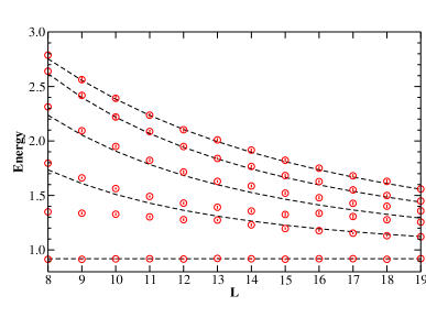
Figure 3: (Left) Spectrum of the theory for different values of the volume for the following simulation parameters: $\nu=1.0$, $\lambda=1.4$, $m_{\pi}=0.36$. The dashed lines describe the free two-particle spectrum. (Right) The interpolated data using a polynomial.

First of all, we interpolate the data for each level using three different polynomials of order 3, 4 and 5 in order to have a relation between the energy $E$ and the side box $L$ in the entire interval $[8,19]$ and to provide a way to evaluate the systematic errors in our final results; in Figure 3 (Right) we show one of these interpolations. In Figures 3, the dashed lines describing the free two-particle spectrum are calculated using Eq. 3. Here we note that the mass $m_{\pi}$ in Eq. 3 is not the bare mass. The value measured on the lattice $m^{ph}_{\pi}=0.460(2)$ is taken as the physical value; the relation between them is well-approximated by $m_{\pi}^{ph}=2\sinh^{-1}(m_{\pi}/2)$.

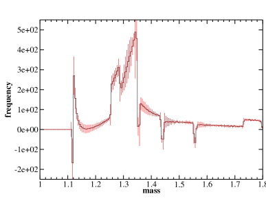
Figure 4: The probability distribution $\tilde{W}=W-W_{0}$ obtained by data from Figure 3.

This free spectrum is used to determine the distribution $W_{0}$ which is then subtracted to $W$ that is obtained from the interacting spectrum. It is important to note that if the number of levels considered to plot $W$ in the interacting spectrum are $N$, then the number of levels we have to consider in the free spectrum to determine $W_{0}$ are just $N-1$.

Using the three previous polynomials we are able to produce a large number of data (we fix $\Delta{L}=0.001$) that we can then use to get the probability distribution $W$ described in Sec 2.4 with the corresponding systematic errors; fixing the bin width to $\Delta{E}=0.005$ we obtain the histogram $\tilde{W}$ of Figure 4. Note that to get $\tilde{W}$ both $W$ and $W_{0}$ are worked out from the same range with $L\in[8,19]$. The error bars in Figure 4 are the results of the systematic errors coming from the histogram $W$ and the statistical errors coming from the histogram $W_{0}$.

Clearly, the shape of the histogram in Figure 4 is far from the Breit-Wigner shape; the reason is related to the fact we are considering only six energy levels but the conclusions of Sec 2.4 are true only in the limit of an infinite number of levels. Moreover a lot on jumps and spikes are present. Our task is now to try to improve this result in order to get more information from our raw data.

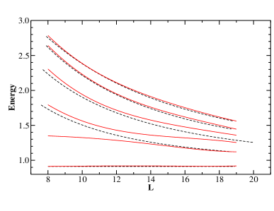
Figure 5: Energy levels of Figure 3 (Right) with the correct free two-particle spectrum background.

We investigated the origin of the spikes and we understood they are related to a “wrong” background $W_{0}$. It is easy to see that the spikes appear every time there is the intersection between the six levels of the interacting spectrum (or of the five levels of the free spectrum) with the extremities of the volume range ($L=8$ and $L=19$). Near those two extremities we have to be careful with what is the correct background; Figure 5 shows a corrected background subtraction. In order to correctly subtract the free background, we lengthen each free spectrum line. This is done so that the extremity of that line has an energy equal to that of the extremity of the interacting spectrum line closest to it. In this way all interacting lines are subtracte correctly rather than the subtraction being affected by the limit of the volume range that we are actually using in our simulations. Using this procedure to determine $W_{0}$ we get the correct histogram of Figure 6 (Left). Unfortunately, in Figure 6 (Left) we continue to see a jump for $E\approx 1.35$; the origin of it can be understood looking at Figure 5. There are two extremity lines, one at $L=8$ and one at $L=19$ (both around $E\approx 1.35$), that are without a “background”; actually, in this case the background is the resonance itself we are looking for. Therefore, there is no way to avoid the presence of this jump because we do not know anything about the resonance; the only thing we can do is to completely exclude from our analysis those two levels, hoping that the resonance can appear. In Figure 6 (Right) we show the probability distribution $\tilde{W}$ in this last case; now clearly a Breit-Wigner shape appears.

It is now possible to fit these data to Eq. 11 to determine the parameters of the resonance; applying a sliding window procedure around the peak, they turn out to be: $M_{\sigma}=1.330(5)$ and $\Gamma_{\sigma}=0.10(5)$.

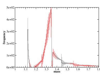
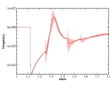
Figure 6: (Left) Probability distribution $\tilde{W}$ obtained by data from Figure 5. (Right) Probability distribution $\tilde{W}$ obtained excluding from the analysis the two levels that in Figure 5 are without a corresponding background.

We have simulated the theory with a second set of parameters, corresponding to a larger width: $\nu=1.0$, $\lambda=4.0$, $m_{\pi}=0.56$. In this case, we tuned them to have the intersection between the $\sigma$ energy level and $(1,0,0)$ two-particle energy level around $L=8$. The physical mass for the pion turns out to be $m^{ph}_{\pi}=0.657(3)$. In Figure 7 (Left) we plot the spectrum for $6\leq L\leq 20$ for the first six levels; the relative error varies in the range 0.05% - 0.2%.

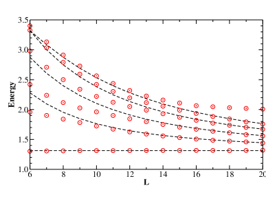
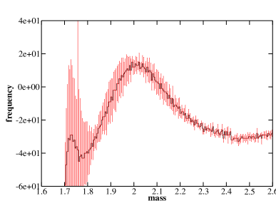
Figure 7: (Left) Spectrum of the theory for different values of the volume for the following simulation parameters:$\nu=1.0$, $\lambda=4.0$, $m_{\pi}=0.56$. (Right) Probability distribution $\tilde{W}$ using the correct background and excluding the two levels that are without a corresponding background.

If we repeat all the procedure as described before (in particular we exclude the two levels which are “without” background) we get the histogram of Figure 7 (Right); also in this case we can clearly see a Breit-Wigner shape and we can fit these data obtaining the following parameters: $M_{\sigma}=2.01(2)$, $\Gamma_{\sigma}=0.35(10)$.

Finally, we have run a third series of simulations with parameters $\nu=1.0$, $\lambda=200.0$, $m_{\pi}=0.86$. They have been tuned to have the intersection between the $\sigma$ energy level and $(2,0,0)$ two-particle energy level around $L=10$. Because in this case we are considering higher momentum, we expect the width of the resonance is larger then the previous cases. In this case we take in account 13 levels to describe better the shape of the resonance. In Figure 8 (Left) the spectrum for $6\leq L\leq 15$ is plotted; the relative error varies in the range 0.15% - 0.4%. The physical mass for the pion turns out to be $m^{ph}_{\pi}=0.938(3)$.

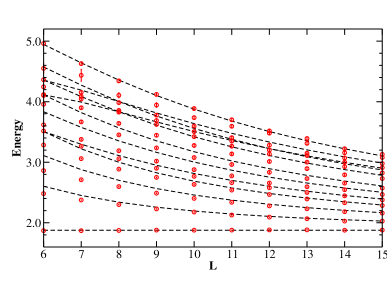
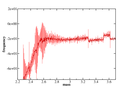
Figure 8: Like Figure 7 but with simulation parameters: $\nu=1.0$, $\lambda=200.0$, $m_{\pi}=0.86$.

Unfortunately, as it is shown in Figure 8 (Right) the probability distribution plot is flat, i.e. no Breit-Wigner shape emerges. It is clear that in this case, the only way to determine the parameters of the resonance is to increase considerably the number of measurements and consequently to decrease the relative errors in the spectrum determination.

In Table 1 a summary of our results for the three sets of parameters are shown.

Relative error in E(L)	$M_{\sigma}$	$\delta(M_{\sigma})/M_{\sigma}$	$\Gamma_{\sigma}$	$\delta(\Gamma_{\sigma})/\Gamma_{\sigma}$
0.5%-1.0%	1.330(5)	0.4%	0.10(5)	50%
0.05%-0.2%	2.01(2)	1.0%	0.35(10)	28%
0.15%-0.4%	–	–	–	–

Table 1: Results for the three sets of simulation parameters with the corresponding relative errors.

In applying Lüscher’s method to the data one only needs the original raw data; there is no need to fit it to a polynomial expression as in the histogram case. The first step is to convert the data on the energy spectrum to data on the momentum spectrum. This requires the dispersion relations. However should it be the lattice or continuum dispersion relations? The lattice dispersion relations are more natural, since they suppress lattice artifacts, but results were obtained for both below to emphasise how much more effective they are.

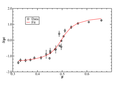
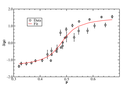
Figure 9: (Left) $\delta(p)$ using Lattice dispersion relations at: $\nu=1.0$, $\lambda=1.4$, $m_{\pi}=0.36$. (Right) Same parameters, but with continuum dispersion relations. Both done with our approximation.

In order to use $p_{n}(L)$ and Eq. 4 to obtain $\delta(p)$, knowledge of $\phi(\kappa)$ is needed. The main difficulty here is the cumbersome definition of $\mathcal{Z}_{js}(1;q^{2})$. Not only that, but as mentioned the summation expansion given above does not even converge in the region required. A more convenient definition is an integral representation of $\mathcal{Z}_{js}(1;q^{2})$ given in Appendix C of Ref [1]. This expression can be used to numerically evaluate $\mathcal{Z}_{js}(1;q^{2})$. Some data on the values of $\phi(\kappa)$ can then be obtained from Eq. 5. We fitted $\phi(\kappa)$ against these values to obtain an approximation of

$$\phi(\kappa)\approx(-0.09937)\kappa^{8}+(0.47809)\kappa^{6}$$ (23)

$$+(-0.62064)\kappa^{4}+(3.38974)\kappa^{2}$$

The error between this approximation and $\phi(\kappa)$ is negligible compared with other errors.

From here we use Eq. 4 to obtain a profile of $\delta(p)$. For the narrow case one can see the difference between use of the continuum dispersion relations and the lattice dispersion relations in Figure 9.

Results
Parameters	$\phi(\kappa)$	$\pi\kappa^{2}$
$\nu=1.0$, $\lambda=1.4$	$M_{\sigma}=1.35(2)$	$M_{\sigma}=1.36(4)$
	$\Gamma_{\sigma}=0.115(8)$	$\Gamma_{\sigma}=0.17(2)$
$\nu=1.0$, $\lambda=4$	$M_{\sigma}=2.03(2)$	$M_{\sigma}=2.2(2)$
	$\Gamma_{\sigma}=0.35(2)$	$\Gamma_{\sigma}=0.42(5)$
$\nu=1.0$, $\lambda=200$	$M_{\sigma}=3.1(7)$	$M_{\sigma}=3(1)$
	$\Gamma_{\sigma}=1.2(5)$	$\Gamma_{\sigma}=2(1)$

Table 2: Resonance mass and decay width using two different approximations for $\phi(\kappa)$.

The lattice dispersion relations provide a tighter fit of the data, as well as having smaller errors. We also compared the use of the traditional approximation of $\phi(\kappa)=\pi\kappa^{2}$ with our approximation. After fitting, the results for the resonance mass and decay width in the two approximations are (both using lattice dispersion relations) shown in Table 2.

The errors are smaller when the approximation of Eq. 4.2 are used, particularly for the broad resonance. It should also be noted that the two approximations effect the two resonance parameters differently. The dispersion relations have a more direct effect on $M_{\sigma}$ while the approximation of $\phi(\kappa)$ has a greater effect on $\Gamma_{\sigma}$.

Results
Parameters	Lüscher’s Method	histogram method
$\nu=1.0$, $\lambda=1.4$	$M_{\sigma}=1.35(2)$	$M_{\sigma}=1.33(5)$
	$\Gamma_{\sigma}=0.115(8)$	$\Gamma_{\sigma}=0.10(5)$
$\nu=1.0$, $\lambda=4$	$M_{\sigma}=2.03(2)$	$M_{\sigma}=2.01(2)$
	$\Gamma_{\sigma}=0.35(2)$	$\Gamma_{\sigma}=0.35(10)$
$\nu=1.0$, $\lambda=200$	$M_{\sigma}=3.1(7)$	$M_{\sigma}=N/A$
	$\Gamma_{\sigma}=1.2(5)$	$\Gamma_{\sigma}=N/A$

Table 3: A comparison between the Lüscher and the histogram method.

This is because a cruder approximation of $\phi(\kappa)$ effects the profile of the scattering phase shift, which is related to the decay width. These results suggested it is optimal to use the lattice dispersion relations and our approximation.

4.3 Comparison between the two methods

The results for Lüscher’s method compared with the histogram method are shown in Table 3.

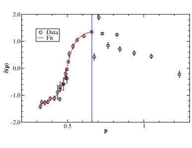
Figure 10: Inelastic data with Lüscher’s formula. For the case of $\nu=1.0$, $\lambda=1.4$. (Onset of inelastic region marked).

Lüscher’s method gives smaller errors than the histogram method, but the results are broadly consistent. Lüscher’s method manages to provide some estimate on the width of the resonance in the broad case.

The broad resonance becomes a problem for the histogram method because there is no obvious peak to indicate the resonance mass (and hence no width of that peak to determine the decay width). One would need very precise data in order to avoid a washing out of the structure of the histogram. Lüscher’s method also becomes more difficult to apply in the case of broad resonances. In the case of a broad resonance the profile of $\delta(p)$ is quite flat, hence a large range of parameters will be capable of fitting to the profile. Again an accurate determination of the energy levels is required to determine the profile precisely enough so that this is prevented. Considering the amount of work necessary before one can use the histogram method (as detailed above), Lüscher’s method is considerably easier to apply, provided one has a good approximation of $\phi(\kappa)$. However, the histogram method can be used as a visual tool for spotting the resonance.

One restriction of Lüscher’s formula is that it only applies in the elastic region. An example of what happens in the inelastic region is provided in Figure 10. It is possible that the histogram method will provide a means of determining the presence of a resonance in the inelastic region. Certainly a histogram can be constructed in the inelastic region, the only difficulty is that with the inapplicability of Lüscher’s formula it is unclear that the parameters of this histogram will have any relation to those of the resonance.

5 Conclusions

We have compared and contrasted the Lüscher and the histogram methods. Lüscher’s method appears to both easier to apply and give smaller errors, however the histogram method does give results consistent with Lüscher’s method and does indeed visually indicate the presence of a resonance.

There are two major difficulties with both methods. First for broad resonances the relevant structure is washed out to some degree. For a histogram, the peak is hard to locate, while for the fit, the profile of the phase shift is poorly constrained. Secondly there is the inelastic region. Lüscher’s formula cannot be used there. The histogram method can be applied to the data, but there is no argument that this is a sensible thing to do. There is also a difficulty in the general case, relevant to QCD, which has not been examined here. In the model above the resonance is clearly present in the channel, since this is an explicit feature of the Lagrangian of the model. In general however a resonance may not be so obvious and there is no reason a priori to expect that it will have a purely Breit-Wigner form.

- [1] M. Lüscher, Nucl. Phys. B 354 (1991) 531.
- [2] V. Bernard, M. Lage, U. G. Meissner and A. Rusetsky, JHEP 0808 (2008) 024 [arXiv:0806.4495 [hep-lat]].
- [3] P. Giudice and M.J. Peardon, AIP Conf. Proc. 1257 (2010) 784.
- [4] C. Morningstar, PoS LATTICE2008 (2008) 009. [arXiv:0810.4448 [hep-lat]].
- [5] M. Lüscher, Nucl. Phys. B 364 (1991) 237.
- [6] M. Lüscher, Comm. Math. Phys. 105 (1986) 153.
- [7] M. Göckeler, H.A. Kastrup, J. Westphalen and F. Zimmermann, Nucl. Phys. B 425 (1994) 413.
- [8] T. DeGrand and C. E. Detar, New Jersey, USA: World Scientific (2006) 345 p.
- [9] M. Lüscher and U. Wolff, Nucl. Phys. B 339 (1990) 222.