Goodput Maximization in Cooperative Networks with ARQ

Abstract

In this paper, the average successful throughput, i.e., $goodput$, of a coded 3-node cooperative network is studied in a Rayleigh fading environment. It is assumed that a simple automatic repeat request (ARQ) technique is employed in the network so that erroneously received codeword is retransmitted until successful delivery. The relay is assumed to operate in either amplify-and-forward (AF) or decode-and-forward (DF) mode. Under these assumptions, retransmission mechanisms and protocols are described, and the average time required to send information successfully is determined. Subsequently, the goodput for both AF and DF relaying is formulated. The tradeoffs and interactions between the goodput, transmission rates, and relay location are investigated and optimal strategies are identified.

I Introduction

In wireless networks, automatic repeat request (ARQ) techniques have been applied to improve the transmission reliability above the physical layer (PHY). Prior work (e.g., in [1] and [2]) has shown that in the PHY of coded or uncoded systems, a higher transmission rate $R$ results in higher packet error rates, leading to more ARQ retransmissions, while a lower $R$ leads to reduced packet error rates and therefore less ARQ retransmissions. Hence, choosing to transmit at very high rates can lead to low average successful throughput (i.e., goodput) due to increased number of retransmissions. On the other hand, transmitting at very low rates leads to more reliable communication but the goodput is also low due to low rates. Consequently, it is of significant interest to jointly optimize the transmission rates (at the physical layer) and the number of ARQ retransmissions (at the data-link layer) by adopting a cross-layer framework so that the goodput of the system is maximized.

In recent years, cooperative operation through relaying has attracted much interest due its promise to improve the link reliability [4] . For instance, when the source-destination link suffers severe fading, information can be sent to the destination through a relay node more reliably if the source-relay and relay-destination channels experience more favorable fading conditions. Note that such diversity achieved through cooperation can also lead to increased goodput. Hence, cooperation is another important tool that can improve the performance.

In this paper, we consider a 3-node cooperative network and investigate the maximization of the goodput in both amplify-and-forward (AF) and decode-and-forward (DF) relaying scenarios. In particular, we investigate the tradeoffs and interactions between the goodput, transmission rates, different ARQ mechanisms, different relaying schemes and relay locations. In both AF and DF modes, we first quantify the link error probabilities through the capacity outage formulation in a coded system in Rayleigh fading channels. Then, we analytically identify the average number of transmissions required for successful delivery, and formulate the goodput of the system. Through numerical results, we study the tradeoffs between the different parameters of the network.

The remainder of this paper is organized as follows. Section II introduces the network model and channel assumptions. Section III presents the goodput analysis in AF and DF cooperative networks with ARQ. Numerical results are given in Section IV. Finally, Section V provides the conclusions.

II System Formulation and Channel Assumptions

We consider a 3-node cooperative network in which the source sends information to the destination with the aid of the relay node. We assume that the source-destination (S-D), source-relay (S-R), and relay-destination (R-D) links experience independent Rayleigh fading.

We have the following key assumptions: 1) channel codes support communication at the instantaneous channel capacity levels, and outages, which occur if transmission rate exceeds the instantaneous channel capacity, lead to packet errors and are perfectly detected at the receivers; 2) depending on whether packets are successfully received or not, ACK or NACK control frames are sent and overheard; 3) ACK/NACK is received reliably with no errors; 4) each codeword contains a certain number of data packets and the transmission of data packets begins when source broadcasts to both relay and destination; 5) the relay mechanism is assumed to be incremental relaying in which the relay node doesn’t need to engage in transmission whenever the S-D link is successful [5],[6].

The ARQ process differs in AF and DF modes. In the AF mode, destination sends ACK when packets are successfully received from the source to notify the source to schedule the next codeword transmission. Otherwise, if source-destination (S-D) link fails, an NACK is sent and relay amplifies and forwards the packets to the destination via the source-relay-destination (S-R-D) cooperative link. If the transmission through the S-R-D link fails as well, destination sends a second NACK and source retransmits the codeword.

In the DF mode, similarly as in AF, it is initially checked whether the transmission through the S-D link is successful. If not, NACK is sent and it is checked whether the relay, which also has to decode the incoming packets and send ACK/NACK frames upon its correct/erronous reception of packets, has received the packets successfully through the source-relay (S-R) link. If the S-R link has also failed, retransmission from the source is requested. If, on the other hand, relay has decoded the packets correctly, relay forwards the packet to the destination. In cases of failure in the relay-destination (R-D) link, retransmissions are requested from the relay. Therefore, retransmissions can be confined only to the R-D link when the relay already has the correct codeword. The network states will be further elaborated in Section III.

II-A Cooperative Network Model

The introduction of a relay node definitely adds more energy overhead and system complexity, but it creates more reliability from the auxiliary R-D link when S-D channel fails. If we assume the signal transmitted from the source is $x$ with unit energy, the received signals at the relay and destination can be represented by

$$y_{s,r}=\sqrt{P_{t}}h_{s,r}x+n_{s,r}$$ (1)

$$y_{s,d}=\sqrt{P_{t}}h_{s,d}x+n_{s,d}$$ (2)

where $P_{t}$ is the transmit power of the source. $h_{s,r}$ and $h_{s,d}$ are channel fading coefficients in the S-R and S-D links, respectively. The fading coefficients are assumed to be zero-mean circularly symmetric Gaussian complex random variables, modeling Rayleigh fading. Path loss is also incorporated into the model through the variance of the fading coefficients. $n_{s,d}$ and $n_{s,r}$ are the additive Gaussian noise components (with variance $N_{0}$) at the destination and relay. We define the SNR at the transmitter side by

$$\gamma=\frac{P_{t}}{N_{0}}.$$

II-B Goodput on a Single Link

Suppose that the source has $J$ codewords to transmit to the destination and the transmission rate is $R$ bits per second. Each codeword has $L$ bits and Codeword(i) needs $X_{i}$ number of transmissions before being successfully received at the destination. The long-term effective throughput on this single link can be formulated by the total transmitted bits over total transmission time [1]. In the limit as $J\rightarrow\infty$, we have

$$\eta=\lim_{J\rightarrow\infty}\frac{JL}{\Sigma_{i=1}^{J}(X_{i}\frac{L}{R})}=\lim_{J\rightarrow\infty}\frac{R}{\frac{1}{J}\Sigma_{i=1}^{J}X_{i}}=\frac{R}{E(X)}.$$ (3)

$X$ is a geometric random variable [1], [7] and $E(X)=\frac{1}{1-\varepsilon}$ where $\varepsilon$ is the link error probability. The link error probability is defined as the probability associated with the outage event on a specific link [4]. For a Rayleigh fading channel, the fading coefficient $h$ is modeled as a zero-mean complex Gaussian random variable with variance $\sigma^{2}$. So $|h|^{2}$ is exponential distributed with mean $\frac{1}{\lambda}=\sigma^{2}$. Therefore, the link error probability for given SNR $\gamma$ and transmission rate $R$ is

$$\varepsilon=P(\log_{2}(1+|h|^{2}\gamma)<R) =P(|h|^{2}<\frac{2^{R}-1}{\gamma})$$

$$=1-e^{(-\frac{2^{R}-1}{\gamma\sigma^{2}})}$$ (4)

III Goodput Analysis with ARQ

III-A Goodput in AF Mode

In the AF mode, relay amplifies and forwards the packets to the destination only if the S-D link is in outage. Hence, there are totally 3 mutually exclusive working states in AF: 1) S-D link is successful; 2) S-D link is in outage, but S-R-D link is successful; 3) both S-D link and S-R-D link are in outage. The source schedules the transmission of the next codeword only after the destination sends back an ACK to announce that the codeword has been successfully received through either State 1 or 2. In State 3, destination sends back an NACK to have the source to retransmit the codeword, triggering ARQ. Consequently, a new transmission round is started all over. This procedure is repeated until a successful codeword delivery is achieved at the destination. The transmission flow is illustrated in Fig. 1 where the red branch denotes the ARQ process.

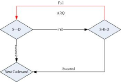
Figure 1: Transmission Flow in AF

We normalize the variance on the S-D link as $\sigma_{s,d}^{2}=1$. From (4), we know the outage probability on the S-D link is

$$\varepsilon_{1} =1-e^{-\frac{2^{R}-1}{\gamma}}.$$ (5)

The variances of the other links are assumed to be proportional to $\sigma^{2}\varpropto d^{-\alpha}$ where $\alpha$ is the path loss coefficient [5]. As for the S-R-D cooperative link, by using a generalized distance factor $k=\frac{d_{s,r}}{d_{s,d}},(k\in(0,1))$, the received SNR via this link can be formulated as

$$\gamma_{s,r,d} =\frac{\gamma|h_{s,r}|^{2}\gamma|h_{r,d}|^{2}}{\gamma|h_{s,r}|^{2}+\gamma|h_{r,d}|^{2}+1}$$

$$=\frac{k^{-\alpha}\gamma|\hat{h}_{1}|^{2}(1-k)^{-\alpha}\gamma|\hat{h}_{2}|^{2}}{k^{-\alpha}\gamma|\hat{h}_{1}|^{2}+(1-k)^{-\alpha}\gamma|\hat{h}_{2}|^{2}+1}.$$ (6)

where $|\hat{h}_{1}|^{2}$ and $|\hat{h}_{2}|^{2}$ are independent random variables with the same distribution as $|h_{s,d}|^{2}$. Note that we implicitly assume with the above formulation that the we have a linear 3-node network where the relay lies in between the source and destination. A more general scenario in which the relay has a certain vertical distance to the line that connects the source and destination can be treated by normalizing $k$ with the cosine of the angle between the source and relay. From [8], we know that $\gamma_{s,r,d}$ has a CDF given by

$$p(\gamma_{s,r,d}<\gamma_{th})=1-\sqrt{\xi}K_{1}(\sqrt{\xi})e^{-\gamma_{th}\left(\frac{k^{\alpha}}{\gamma}+\frac{(1-k)^{\alpha}}{\gamma}\right)}$$ (7)

where $\xi=\frac{4(\gamma_{th}^{2}+\gamma_{th})}{\gamma^{2}(k(1-k))^{-\alpha}}$ and $K_{1}()$ is the first order modified Bessel function of the second type. Hence, the outage probability on the S-R-D link is

$$\varepsilon_{2}=1-\sqrt{\xi}K_{1}\left(\sqrt{\xi}\right)e^{-(2^{R}-1)\left(\frac{k^{\alpha}}{\gamma}+\frac{(1-k)^{\alpha}}{\gamma}\right)}$$ (8)

where $\xi=\frac{4((2^{R}-1)^{2}+(2^{R}-1))}{\gamma^{2}(k(1-k))^{-\alpha}}$. Now, the probabilities of the 3 network states of the AF mode are

$$p_{1} =1-\varepsilon_{1}$$ (9)

$$p_{2} =\varepsilon_{1}(1-\varepsilon_{2})$$ (10)

$$p_{3} =\varepsilon_{1}\varepsilon_{2}.$$ (11)

We define $T=\frac{L}{R}$ as the time required to transmit one codeword over any link. In State 1, a duration of $T$ is needed. At the end of this period, successful transmission is achieved. In both States 2 and 3, a duration of $2T$ is needed. In the first $T$ seconds, source transmits. Since the S-D link fails in these two states, the relay engages in transmission in the following $T$ seconds. As demonstrated in (3), goodput is obtained by first determining the average number of transmissions or equivalently the average time required to send one codeword to the destination successfully. Next result provides the average time in the AF scenario.

Proposition 1

In AF relaying under the ARQ retransmission scheme with 3 states described in this section, the average time needed to successfully transmit one codeword from the source to the destination is given by

$$T_{AF}=\frac{Tp_{1}+2Tp_{2}+2Tp_{3}}{1-p_{3}}.$$ (12)

where $p_{1},p_{2},$ and $p_{3}$ are given in (9) – (11), and $T$ is the time needed to transmit one codeword in one attempt over any link.

Proof See Appendix -A.

The goodput in AF networks is defined as the ratio of $L$ bits (i.e., the number of information bits in each codeword) to the average time required to successfully send one codeword:

$$\eta_{AF} =\frac{L}{T_{AF}}=\frac{R(1-p_{3})}{p_{1}+2p_{2}+2p_{3}}=\frac{R(1-\varepsilon_{1}\varepsilon_{2})}{1+\varepsilon_{1}}$$

$$=\frac{R(1-(1-e^{-\frac{2^{R}-1}{\gamma}})(1-\sqrt{\xi}K_{1}\left(\sqrt{\xi}\right)e^{\frac{-(2^{R}-1)}{\frac{\gamma}{k^{\alpha}+(1-k)^{\alpha}}}}))}{2-e^{-\frac{2^{R}-1}{\gamma}}}.$$ (13)

where $R$ is the transmission rate in bits/s. The following result identifies the optimal $k$ that maximizes the goodput, and shows that the relay should be located halfway between the source and destination.

Proposition 2

For any given transmission rate $R$ and SNR $\gamma$, the AF goodput $\eta_{AF}$ is maximized at $k=0.5$.

Proof: We first note that $\sqrt{\xi}K_{1}(\sqrt{\xi})$ is a monotonically decreasing positive function of $\xi$, and $\xi$ monotonically increases as $k(1-k)$ increases where $k\in(0,1)$. Hence, $\sqrt{\xi}K_{1}(\sqrt{\xi})$ is minimized when $k(1-k)$ is maximized at $k=0.5$. Moreover, $e^{\frac{-(2^{R}-1)}{\frac{\gamma}{k^{\alpha}+(1-k)^{\alpha}}}}$ monotonically decreases as $k^{\alpha}+(1-k)^{\alpha}$ decreases. The function $f(k)=k^{\alpha}+(1-k)^{\alpha}$ with $\alpha>1$ is minimized at $k=0.5$. Therefore, $e^{\frac{-(2^{R}-1)}{\frac{\gamma}{k^{\alpha}+(1-k)^{\alpha}}}}$ is minimized at $k=0.5$. Hence, $\sqrt{\xi}K_{1}\left(\sqrt{\xi}\right)e^{\frac{-(2^{R}-1)}{\frac{\gamma}{k^{\alpha}+(1-k)^{\alpha}}}}$ is minimized and $\eta_{AF}$ is maximized at $k=0.5$ regardless of the values of $R$ and $\gamma$. $\square$

III-B Goodput in DF Mode

In the DF mode, relay forwards the packets to the destination only if the S-D link is in outage and S-R link is successful. So, there are 4 mutually exclusive working states in the DF mode with the following ACK/NACK feedback schemes: 1) S-D link is successful and destination sends back ACK to have the source to send the next codeword; 2) both the S-D and S-R links are in outage and both send back NACKs to request the source to retransmit the codeword; 3) S-D link is in outage, but S-R and R-D links are successful, and source transmits the next codeword in the next block after receiving ACK from the destination; 4. S-D link is in outage, S-R link is successful, but R-D link is in outage. In this state, destination sends an NACK but requests retransmissions from the relay since the relay has successfully decoded the codeword. Hereby, we see two different types of ARQ retransmissions. In State 2, source receives NACKs from both relay and destination and then retransmits, which could be considered as an outer-loop ARQ. In State 4, relay retransmits to the destination, and this could be considered as an inner-loop ARQ. The inner-loop is beneficial when the relay is closer to the destination than the source is. The transmission flow can be seen in Fig. 2.

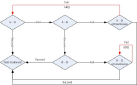
Figure 2: Transmission Flow in DF

Again we normalize the variance on the S-D link as $\sigma_{s,d}^{2}=1$ and by using a generalized distance factor $k=\frac{d_{s,r}}{d_{s,d}},(k\in(0,1))$, we have the following outage probabilities on the S-D, S-R and R-D links, respectively,

$$\varepsilon_{1} =1-e^{(-\frac{2^{R}-1}{\gamma})}$$ (14)

$$\varepsilon_{2} =1-e^{(-\frac{k^{\alpha}(2^{R}-1)}{\gamma})}$$ (15)

$$\varepsilon_{3} =1-e^{(-\frac{(1-k)^{\alpha}(2^{R}-1)}{\gamma})}.$$ (16)

Now, the probabilities of the 4 states are given by

$$p_{1} =1-\varepsilon_{1}$$ (17)

$$p_{2} =\varepsilon_{1}\varepsilon_{2}$$ (18)

$$p_{3} =\varepsilon_{1}(1-\varepsilon_{2})(1-\varepsilon_{3})$$ (19)

$$p_{4} =\varepsilon_{1}(1-\varepsilon_{2})\varepsilon_{3}.$$ (20)

Similarly as in the AF case, we first determine the average time needed to successfully transmit one codeword.

Proposition 3

In DF relaying under the ARQ retransmission scheme with 4 above-described states, the average time needed for the successful transmission of one codeword is

$$T_{DF}=\frac{Tp_{1}+Tp_{2}+2Tp_{3}+(2+\frac{1}{1-\varepsilon_{3}})Tp_{4}}{1-p_{2}}.$$ (21)

Proof: See Appendix -B.

Hence, the goodput is

$$\eta_{DF}=\frac{L}{T_{DF}}=\frac{R(1-p_{2})}{p_{1}+p_{2}+2p_{3}+(2+\frac{1}{1-\varepsilon_{3}})p_{4}}.$$ (22)

IV Numerical Results

In this section, we present the numerical results. In particular, we compute the goodput in AF and DF relaying scenarios by using the expressions in (13) and (22) and investigate the network performance as the transmission rate $R$, normalized relay location $k$, and SNR $\gamma$ vary.

We first look at $\eta_{AF}$ (goodput in the AF mode) as a function of $R$ with $\gamma=10dB$ and $\alpha=3.12$ [9]. The upper subplot in Fig. 3 clearly shows for any given normalized relay location $k$, goodput is maximized at a certain unique optimal rate $R^{*}$. At rates below $R^{*}$, even though the link reliabilities are comparatively high, $\eta_{AF}$ is low due to small $R$. At rates higher than $R^{*}$, the decrease in link reliability and increased number of retransmissions counteracts the increased rate, resulting again in lower $\eta_{AF}$. Similar results are also observed in the lower subplot, which plots the goodput $\eta_{DF}$ in the DF mode with respect to transmission rate $R$.

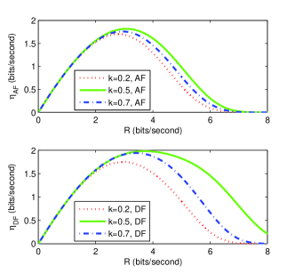
Figure 3: Goodput $\eta$ vs $R$

In Fig. 4, we fix the transmission rate $R$ at different values and plot the goodput $\eta$ for both AF and DF as a function of the normalized relay location $k$. Verifying the result of Proposition 2, we observe that the AF goodput $\eta_{AF}$ is optimized at $k=0.5$ regardless of the value of $R$. In DF, the optimal relay location is close to $k=0.5$ for large values of $R$. However, we see that when $R$ is relatively low (i.e., when $R=4$ bits/s), $k$ is slightly larger than 0.5 meaning that relay should be placed farther away from the source and closer to the destination. Note also that a higher goodput is achieved when $R=4$ bits/s. Finally, we observe that at the optimal relay location, DF relaying provides higher goodput than AF relaying for the same transmission rate.

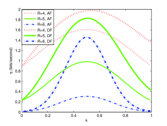
Figure 4: Goodput $\eta$ vs Relay Location $k$

In Fig. 5, we plot $\eta$ as a function of $R$ at different SNR values in both AF and DF when the generalized relay location is set at $k=0.5$. When SNR is maintained at a moderate level, DF outperforms AF in terms of providing higher goodput at any transmission rate. At very high SNR, AF and DF modes have almost identical performance curves. Since the link reliability is so high that very few ARQ rounds are needed to achieve the successful packet delivery, the goodput is actually approaching the transmission rate $R$. Secondly, in either mode, we see as $\gamma$ increases, the optimal goodput $\eta^{*}$ and $R^{*}$ which maximizes $\eta$ are both increasing.

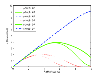
Figure 5: Goodput $\eta$ vs $R$ at Different SNR

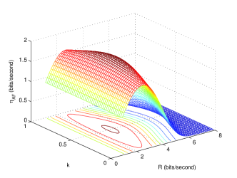
Figure 6: Goodput vs $k$ and $R$ in AF

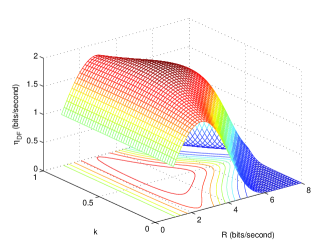
Figure 7: Goodput vs $k$ and $R$ in DF

In Fig. 6 and Fig. 7, the goodput is plotted as both the relay location and transmission rate are varied. It is assumed that SNR $\gamma=10dB$. As is shown in the contours, the goodput surface isn’t ideally concave, but there is always a pair of optimal relay location $k^{*}$ and transmission rate $R^{*}$ that maximizes the goodput.

In Fig. 8 , we assume $\gamma=10dB$ and plot the optimal $k*$ and the optimal goodput $\eta^{*}$ as a function of the transmission rate $R$ in both AF and DF. The upper subplot confirms again the result in Proposition 2 and shows that $k^{*}=0.5$ in AF. In the DF mode, we see that $k^{*}$ decreases from 1 and approaches 0.5 asymptotically as $R$ increases, which is in compliance with our observation in Fig. 4. In the lower subplot, the optimal goodput $\eta^{*}$ achieved at the optimal $k^{*}$ is shown, where we see that DF outperforms AF and provides higher goodput for any given transmission rate $R$.

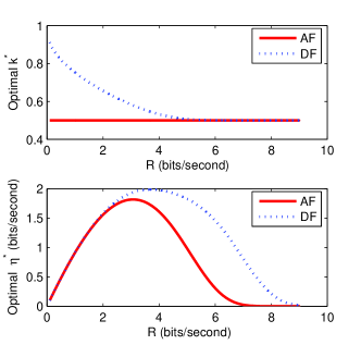
Figure 8: Optimal Relay Location and Goodput vs $R$

V Conclusion

In this paper, we have performed a cross-layer optimization to maximize the goodput of cooperative networks that employ ARQ schemes and work in either AF or DF relaying mode. For both AF and DF schemes, we have described the retransmission mechanisms and determined the average time required to send the information correctly from the source to the destination. Subsequently, we have formulated the goodput achieved in both relaying modes. We investigated the impact of transmission rates and relay location on the goodput. We have shown that having the relay halfway between the source and destination maximizes the goodput. Through numerical results, we have identified the optimal transmission rates that maximize the goodput. We have also numerically analyzed the optimal relay location in DF. We have shown that DF generally provides superior performance.

-A Proof of Proposition 1

In the AF mode, we have three networks states and the ARQ is triggered when both S-D and S-R-D links fail. Therefore, the transmission flow can be illustrated as a tree structure as depicted in Fig. 9 as the ARQ round progresses.

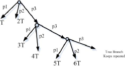
Figure 9: Transmission Tree Structure in AF

Each branch corresponds to a time consumption with a certain probability. We model the time required to successfully transmit one codeword as a random variable and denote it as $X$. It can be easily seen that $X$ has the following distribution by

$$X=\left\{\begin{array}[]{ll}T,&\text{$p_{1}$}\\ 2T,&\text{$p_{2}$}\\ 3T,&\text{$p_{3}p_{1}$}\\ 4T,&\text{$p_{3}p_{2}$}\\ 5T,&\text{$p_{3}^{2}p_{1}$}\\ 6T,&\text{$p_{3}^{2}p_{2}$}\\ \vdots\end{array}\right.$$ (30)

For odd number of time slots, the probability distribution is

$$p((2k+1)T)=\begin{array}[]{ll}p_{3}^{k}p_{1},&\text{ for $k=0,1,2\cdots$}\\ \end{array}$$ (32)

For even number of time slots, the probability distribution is

$$p((2k+2)T)=\begin{array}[]{ll}p_{3}^{k}p_{2},&\text{ for $k=0,1,2\cdots$}\\ \end{array}$$ (34)

So, the average time $E(X)=T_{AF}$ is

$$T_{AF} =\sum_{k=0}^{\infty}(2k+1)Tp_{3}^{k}p_{1}+\sum_{k=0}^{\infty}(2k+2)Tp_{3}^{k}p_{2}$$

$$=T\left[p_{1}(\frac{2p_{3}}{(1-p_{3})^{2}}+\frac{1}{1-p_{3}})+2p_{2}(\frac{p_{3}}{(1-p_{3})^{2}}+\frac{1}{1-p_{3}})\right]$$

$$=\frac{(p_{1}+2p_{2}+2p_{3})T}{1-p_{3}}.$$ (35)

$\square$

-B Proof of Proposition 3

In the DF mode, the transmission flow can be illustrated as in Fig. 10, where the long branches occurring with probability $\varepsilon_{1}\varepsilon_{2}$ and extending to the right are generated when the outer ARQ round is triggered. Recall that the outer ARQ is triggered when both S-R and S-D links fail, requiring the source to retransmit. Note that there is also a downward progression starting initially with probability $\varepsilon_{1}(1-\varepsilon_{2})$. This progression occurs when the inner ARQ rounds are triggered, in which relay, having received the packets successfully from the source, retransmits when the R-D link fails.

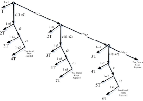
Figure 10: Transmission Tree Structure in DF

In DF relaying, the random variable $X$, which is time required to one codeword successfully, can be expressed as

$$X=\left\{\begin{array}[]{ll}T,&\text{$1-e_{1}$}\\ Y_{1},&\text{$\varepsilon_{1}(1-\varepsilon_{2})$}\\ Z_{1},&\text{$\varepsilon_{1}\varepsilon_{2}$}\end{array}\right.$$ (39)

where $Y_{1}$ and $Z_{1}$ are also random variables whose distributions are as follows:

$$Y_{1}=\left\{\begin{array}[]{ll}2T,&\text{$1-\varepsilon_{3}$}\\ 3T,&\text{$\varepsilon_{3}(1-\varepsilon_{3})$}\\ \vdots\\ nT,&\text{$\varepsilon_{3}^{n-2}(1-\varepsilon_{3})$}\end{array}\right.,\quad Z_{1}=\left\{\begin{array}[]{ll}2T,&\text{$1-\varepsilon_{1}$}\\ Y_{2},&\text{$\varepsilon_{1}(1-\varepsilon_{2})$}\\ Z_{2},&\text{$\varepsilon_{1}\varepsilon_{2}$}\end{array}\right..$$ (47)

Above, we have defined

$$Y_{2}=\left\{\begin{array}[]{ll}3T,&\text{$1-\varepsilon_{3}$}\\ 4T,&\text{$\varepsilon_{3}(1-\varepsilon_{3})$}\\ \vdots\\ nT,&\text{$\varepsilon_{3}^{n-3}(1-\varepsilon_{3})$}\end{array}\right..$$ (52)

$Z_{2}$ can be defined similarly as $Z_{1}$ but now in terms of $Y_{3}$ and $Z_{3}$. Repeating this procedure, we have random variables defined in a nested fashion with a certain pattern. By examining the characteristics of $Y_{k}$, we can easily find its mean value as

$$E(Y_{k})=(1-\varepsilon_{3})T\left(\frac{\varepsilon_{3}}{(1-\varepsilon_{3})^{2}}+\frac{k+1}{1-\varepsilon_{3}}\right).$$ (53)

Now, the expected value of $X$ is

$$E(X)= (1-\varepsilon_{1})T+\varepsilon_{1}(1-\varepsilon_{2})E(Y_{1})+\varepsilon_{1}\varepsilon_{2}E(Z_{1})$$

$$= (1-\varepsilon_{1})T+\varepsilon_{1}(1-\varepsilon_{2})E(Y_{1})+\varepsilon_{1}\varepsilon_{2}\cdot$$

$$[(1-\varepsilon_{1})2T+\varepsilon_{1}(1-\varepsilon_{2})E(Y_{2})+\varepsilon_{1}\varepsilon_{2}\cdot$$

$$\left((1-\varepsilon_{1})3T+\varepsilon_{1}(1-\varepsilon_{2})E(Y_{3})+\varepsilon_{1}\varepsilon_{2}E(Z_{3})\right)]$$

$$= \sum_{k=0}^{\infty}(\varepsilon_{1}\varepsilon_{2})^{k}(1-\varepsilon_{1})(k+1)T+\sum_{k=0}^{\infty}(\varepsilon_{1}\varepsilon_{2})^{k}\varepsilon_{1}(1-\varepsilon_{2})E(Y_{k+1})$$

$$= \frac{T(1-\varepsilon_{1}\varepsilon_{2})(1+\varepsilon_{1}-\varepsilon_{3}-\varepsilon_{1}\varepsilon_{2})}{(1-\varepsilon_{1}\varepsilon_{2})^{2}(1-\varepsilon_{3})}$$

$$= \frac{Tp_{1}+Tp_{2}+2Tp_{3}+(2+\frac{1}{1-\varepsilon_{3}})Tp_{4}}{1-p_{2}}.$$ (54)

$\square$

References

- [1] P. Wu, N. Jindal, “Coding versus ARQ in fading channels: How reliable should the PHY be?”, Globecom 2009.
- [2] R. Aggarwal, P. Schniter, and C. Koksal,“Rate adaptation via linklayer feedback for goodput maximization over a time-varying channel,” IEEE Trans. Wireless Commun., Vol.8, No.8, 2008.
- [3] T. H. Himsoon, W. P. Siriwongpairat, Z. Han, K. J. Ray Liu, “Lifetime maximization via cooperative nodes and relay deployment in wireless networks”, IEEE Journal on Selected Areas in Communications, Vol.25, No. 2, Feb. 2007
- [4] K. J. Ray Liu, A. K . Sadek, W. Su, A. Kwasinski, Cooperative Communications and Networking, Cambridge University Press, 2009.
- [5] T. Renk, H. Jakel, F. K. Jondral, D. Gunduz, A. Goldsmith, “Outage capacity of incremental relaying at low signal-to-noise ratios”, IEEE Vehicular Technology Conference (VTC), Anchorage, AK, Sep. 2009.
- [6] W. Choi, D. I. Kim, B-H. Kim, “Adaptive multi-node incremental relaying for hybrid-ARQ in AF relay networks”, IEEE Trans. on Wireless Communication, Vol. 9, No. 2, Feb. 2010.
- [7] S. Banerjee and A. Misra, “Minimum energy paths for reliable communication in multi-hop wireless networks,” MOBIHOC, pp.146-156, June. 2002.
- [8] M. O. Hasna, M. S. Alouini, “End-to-end performance of transmission systems with relay over Rayleigh-fading channel”, IEEE Transaction on Wireless Communication, Vol. 2, No. 6, Nov 2003.
- [9] V. Erceg, L. J. Greenstein, S. Y. Tjandra, S. R. Parkoff, A. Gupta, B. Kulic, A. A. Julius, and R. Bianchi, “An emperically based path loss model for wireless channels in suburban environments,” IEEE J.Select. Areas Commun, Vol. 17, No. 7, pp.1205-1211, Jul. 1999.