Constraining properties of the black hole population using LISA
Abstract
LISA will detect gravitational waves from tens to hundreds of systems containing black holes with mass in the range –. Black holes in this mass range are not well constrained by current electromagnetic observations, so LISA could significantly enhance our understanding of the astrophysics of such systems. In this paper, we describe a framework for combining LISA observations to make statements about massive black hole populations. We summarise the constraints that LISA observations of extreme-mass-ratio inspirals might be able to place on the mass function of black holes in the LISA range. We also describe how LISA observations can be used to choose between different models for the hierarchical growth of structure in the early Universe. We consider four models that differ in their prescription for the initial mass distribution of black hole seeds, and in the efficiency of accretion onto the black holes. We show that with as little as 3 months of LISA data we can clearly distinguish between these models, even under relatively pessimistic assumptions about the performance of the detector and our knowledge of the gravitational waveforms.
1 Introduction
Current measurements of black hole (BH) masses are almost exclusively for systems with mass above . The shape of the mass function for less massive BHs is expected to retain a signature of the initial mass distribution of the seeds from which BHs grow, which is erased at the high mass end by the effects of accretion [1]. In addition, it is not known if the tight correlations observed between the properties of high mass BHs and their host galaxies extend down to lower masses [2], which has important consequences for our understanding of the co-evolution of galaxies and BHs. Probing BHs in the mass range is thus crucial to our understanding of the growth of structure, and LISA [3] is one of the few instruments that has the potential to observe such systems. LISA is expected to see a few tens of massive BH mergers (MBHMs) per year [4, 6] and as many as several hundred extreme-mass-ratio inspirals (EMRIs) of stellar-mass compact objects into massive BHs in the centres of galaxies [5]. The MBHMs can be observed throughout the Universe, while the EMRIs will only be seen at low redshift, , but LISA will be able to measure the parameters of both kinds of event to unprecedented precision [6, 7, 8].
The mass function of BHs in the LISA range is uncertain due to the lack of direct observations. If the BH population traces the active galaxy population, then the mass function should turn over for [9]. However, if the L– and M– relations derived for more massive galaxies can be extrapolated to lower masses, the observed galaxy luminosity function would imply a flat BH mass function in this range [9]. Applying corrections to Sloan Digital Sky Survey measurements of the velocity dispersion instead yields a mass function that increases toward lower masses [10]. Overall the present uncertainty in the slope of the quiescent BH mass function for is at least [11]. LISA EMRI observations could therefore play an important role in pinning down this slope in the low-redshift Universe.
LISA MBHM events will occur following mergers of the host galaxies of the BHs, and thus trace the hierarchical growth of structure. Models of structure formation are tuned to match existing observations, and therefore make similar predictions for mergers at the high mass end of the BH mass function, but differ significantly for lower masses. In particular, both “light seed” [12] and “heavy seed” [13] models are consistent with existing data. It is unlikely that observations in the electromagnetic spectrum will rule out either class of models in the next decade, so LISA could make important contributions to our understanding of the early epoch of galaxy formation.
LISA will be able to make very precise measurements of the parameters of individual EMRI and MBHM systems that are observed [7, 8, 6]. Precise measurements for single systems are very important for fundamental physics [14], but it is the full set of events that are seen which will carry the most important information for astrophysics. In this paper, we describe a method to combine this information in order to make astrophysical statements, which is based on a Bayesian framework using a parametric model for the probability distribution of observed events. LISA model selection using MBHMs was also considered in [15] using the non-parametric Kolmogorov-Smirnov test to compare parameter distributions. While our conclusions are broadly similar, the framework presented here is more general and can be easily extended to other problems.
This paper is organised as follows. In Section 2 we describe our approach to using LISA to place constraints on astrophysical models. This includes a discussion of the statistical framework used for model selection and a description of how we model LISA instrumental effects, i.e., the completeness of LISA observations and the parameter estimation errors that arise from noise in the detector. In Section 3.1 we summarise the constraints that LISA EMRI observations could place on the shape of the BH mass function in the LISA range. These results were previously described in [11] but we briefly review them here for completeness. In Section 3.2 we describe how LISA can be used to choose between different models for the hierarchical growth of structure. We illustrate this using four different models that differ in their seed mass distributions and accretion prescriptions. These results are new and appear here for the first time. In Section 4 we discuss our results and possible extensions of this work.
2 Methods
Our aim is to make inferences about the population of BHs in the Universe based on LISA observations. Bayes theorem relates the posterior probability, , for the parameters of a model given observed data , to the likelihood of seeing that data under model with parameters , and the prior, for the parameters :
| (1) |
In this context, the model is a description of the population of BHs in the Universe, the data are the parameters of the sources that LISA detects and the uncertainty in the distributions comes from the fact that mergers occur stochastically in the Universe — a given model will predict the rate at which LISA events occur but cannot predict the exact systems that LISA will observe.
To compute the likelihood, , we can imagine dividing the parameter space of possible signals into bins, labelled by . The data, , is the number of events, , observed in each bin . A particular model will predict the rate, , at which events in a particular parameter bin occur in the Universe. As the events start at random times, the number of events occurring in a given bin during the LISA mission will be drawn from a Poisson probability distribution with rate . Events in different bins are independent and so if we temporarily ignore LISA selection effects and parameter estimation errors, the likelihood of seeing the set of events , is
| (2) |
It is possible to take the continuum limit of this expression by letting the bin volume approach zero. The above expression then becomes a product of the point probabilities of the events observed, normalised by the total number of events the model predicts.
For model selection, i.e., to choose the model that provides the best description of the observed data, we use the evidence, which is the quantity appearing in the denominator of Bayes Theorem, Eq. (1). To compare models A and B, we compute the odds ratio (see, for example, [16])
| (3) |
in which denotes the prior probability assigned to model . If (), model (model B) provides a much better description of the data.
The fact that we use an imperfect detector to make the observations introduces two complications into the analysis. Firstly, the data set is not complete — LISA sees only a certain subset of the events that occur during the mission. Secondly, the presence of noise in the detector introduces errors into the parameter estimates.
The incompleteness of the LISA observation means that only a certain fraction of the events that occur in a given bin in the parameter space will be detected. If the completeness is known as a function of the source parameters, then this can be included in the likelihood computation by replacing by the effective observed rate, , in Eq. (2), where is the completeness in bin . In our analysis, we assume a simple signal-to-noise ratio (SNR) cut model for completeness. We assume that of events with matched-filtering SNR are detected, and that of events with are detected. This is a reasonable model if is set moderately high, since if events with SNR less than were actually detected, they could just be excluded from the analysis. The parameters of events with lower SNR tend to be more poorly determined and thus do not contribute much to model discrimination, so there is little change in the results when such events are excluded.
Instrumental noise leads to imperfect parameter measurement. In the analysis of actual LISA data, we will derive a posterior probability distribution (pdf) for the parameters of the sources. Using this, the likelihood can be obtained by integrating the continuum version of Eq. (2) over the pdf [11]. An equivalent approach, which is more convenient for scoping out LISA’s potential, is to suppose each source is assigned to the bin in which the maximum a posteriori probability lies, and to fold the parameter uncertainty into the effective rate of observed events, , in each bin. In practice, can be computed by generating a large number of realisations of the set of events that LISA observes. For each event in each realisation the parameter uncertainty may be modelled as a Gaussian, , centred on the true parameters, . A fractional rate is assigned to each bin . This is similar in principle to the LISA “error kernel” described in [17]. The parameter error comes primarily from detector noise, but additional errors arise from weak lensing, which changes the apparent luminosity distance of sources at higher redshift, and from uncertainties in the cosmological parameters used to convert from luminosity distance to redshift. These can be included in the redshift-redshift component of by writing , where , , cos denote the contributions from noise, weak-lensing and cosmological parameter uncertainty. We model the weak-lensing error using results in [18] and the cosmological error following [19]:
| (4) |
and we assume that by the time LISA flies.
3 Results
3.1 Extreme-mass-ratio inspirals
This preceding framework was used in [11] to explore the constraints that LISA EMRI observations could place on the BH mass function at low redshift. This analysis made various assumptions — an SNR cut of was used to define the completeness function; all EMRIs were assumed to be on circular and equatorial orbits, which meant the completeness could be determined from the observable lifetime of a particular EMRI, as defined in [5]; parameter estimation errors were ignored in the analysis, but included in the generation of realisations of the LISA data; the data was taken to be measurements of the central BH mass and source redshift only; and the scaling of the intrinsic EMRI rate per BH was assumed to be known and given by results in [20]. Assuming a simple power-law mass function, , and that all BHs have spin , it was found that LISA could measure the parameters to a precision and if events were observed. This compares very well to the current precision, , on the slope of the BH mass function, particularly given that these models typically predict s of observable EMRI events.
Using a redshift-dependent ansatz for the mass function, , it was found that LISA would not be able to place reasonable constraints on the evolution parameters , . This is because the majority of EMRI events will be detected at low redshift, . The main caveat in these results is the assumption that the mass-dependence of the EMRI rate will be known by the time LISA flies. These results can also be interpreted as the precision with which the convolution of the mass function with the EMRI rate can be determined. More work is required to determine if combined EMRI and MBHM observations can decouple these effects and perhaps measure evolution in the mass function.
3.2 Comparable mass black hole mergers
LISA observations of MBHMs can be used to choose between different models for the growth of structure. There are various models for the hierarchical assembly of galaxies, but these have been tuned to fit existing electromagnetic observations which do not constrain BHs in the mass range of interest to LISA. The models therefore make quite different predictions for the expected set of LISA events, which means that LISA has the potential to discriminate between them. We consider four different models, which differ in the prescription for the masses of the initial seeds from which BHs grow and in the prescription for accretion onto the BHs. We consider two “light seed” models [12], in which BH seeds of mass form as remnants of metal-free stars at redshift , and two “heavy seed” models [13], in which seeds with mass form directly from the collapse of massive protogalactic disks in the redshift range . In each case, we consider two accretion prescriptions [21]: (i) “coherent” accretion, in which material accreting onto the black hole tends to have similar angular momentum [22, 23], which could occur if the large scale structure of the feeding material is in a disc-like configuration [24, 25]; (ii) “chaotic” accretion, in which there are many short accretion episodes with different angular momentum spin axes in each one [26]. The four models are summarised in Table 1. We chose these four models to allow easier comparison to the literature. The same four models were used to explore LISA parameter estimation [6] and in previous work on using LISA for model selection [15]. The accretion model primarily leads to different expectations for the black hole spins (intermediate-high, , in the coherent case; low, , in the chaotic case). In this work we ignore black hole spin, but the accretion prescription also leaves an imprint on the component masses. The models assume that the mass-to-energy conversion efficiency, , depends on black hole spin only, so the two models predict different average efficiencies of and respectively. The mass-to-energy conversion directly affects mass growth, with high efficiency implying slow growth, since for a black hole accreting at the Eddington rate, the black hole mass increases with time as
| (5) |
where Gyr. The “coherent” versus “chaotic” models thus allow us to study how different growth rates affect LISA observations.
| Model | Seed mass prescription | Accretion prescription | LISA events per year |
|---|---|---|---|
| SE | VHM (light seeds) | coherent | 37 (18) |
| SC | VHM (light seeds) | chaotic | 40 (21) |
| LE | BVR (heavy seeds) | coherent | 24 (22) |
| LC | BVR (heavy seeds) | chaotic | 21 (18) |
We will again use an SNR cut, , to characterise whether an event is detectable or not, and we will make both optimistic and pessimistic assumptions about LISA in terms of the number of data streams that are available for data analysis. At low frequency two independent data streams can be constructed from the data stream of a single LISA constellation, but one of these data streams could be lost if there is a failure on one of the three satellites in the constellation. We will therefore consider four possible scenarios: (i) 1 independent data stream, ; (ii) 1 independent data stream, ; (iii) 2 independent data streams, ; (iv) 2 independent data streams, . Scenarios (ii)/(iii) are the most pessimistic/optimistic. Additionally, we include only systems that merge within the LISA observation window in the analysis, and we consider five different possible lengths of the LISA data set used in the analysis (3 months, 6 months, 1 year, 18 months and 2 years). It is unlikely that LISA will only take data for a few months if it works at all, but these results illustrate what we will be able to say after 3 months of observation, after 6 months and so on.
To carry out model selection, we must compute the likelihood of the data under the various models, as given by Eq. (2). For the current analysis, we use only three parameters to characterise each system: the total mass, , the mass ratio, , and the source redshift, . We compute the expected rate of observed events in each bin accounting for errors in the parameter estimation as described in Section 2. We compute parameter estimation errors using the Fisher matrix approximation for quasicircular, non-spinning BH binary inspirals modelled in the restricted post-Newtonian approximation, following [19]. Cosmological parameter uncertainties and weak lensing errors are folded in as described above. The fact that we are ignoring spins, eccentricity and higher harmonics in our analysis has two consequences. Firstly, our estimates for the signal-to-noise ratio for each source are pessimistic, because spins and higher harmonics of the signal (which are neglected in our model) usually increase the energy radiated and the mass reach of the detector. Secondly, spin encodes important information about the history of a particular BH, and in particular its accretion history [21]. This could help resolve models where BHs are “born equal” but grow via different mechanisms. In this sense our results should be considered conservative.
The four models we use do not have free parameters, so we cannot determine a posterior probability distribution on the model parameters. Instead, we can use Eq. (3) to decide which model provides the best description of the data. The models we are comparing have all been constructed to be consistent with existing constraints from observations in the electromagnetic spectrum, so there is presently no reason to prefer one model over the others. We therefore assume equal prior probabilities on all models, so the odds ratio reduces to the likelihood ratio
| (6) |
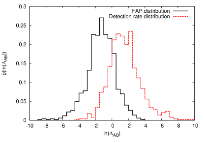
It is clear that when , model should be preferred. What value of is sufficient to make such a statement? This can be answered by looking at the distribution of over many realisations of model and model . We generate a realisation of model by drawing events from the underlying population, applying the appropriate SNR cut, and adding in parameter errors to each event. We can then compute the likelihoods for this event set under model and model and hence . In Figure 1 we show the distribution of in 1000 realisations each of model and model .
 |
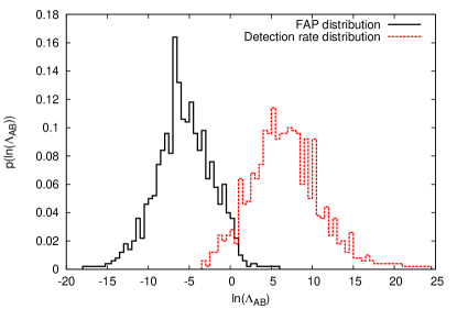 |
As we would expect, when the realisation is drawn from model , tends to be greater than , while when it is drawn from model , tends to be less than . For a given choice of threshold on , points in the model histogram to the right of that threshold represent “detections”, i.e., realisations in which model would be chosen over model when model was correct. Points in the model histogram are “false alarms”, i.e., realisations in which model is chosen over model when in fact model is correct. The histograms become better separated when using a longer segment of LISA data, since we have more events in that case. Another way to represent this information is through a receiver-operator-characteristic (ROC) curve, which shows “detection” probability versus “false alarm” probability (FAP). For a given threshold on , the detection probability is the fraction of realisations of model that lie to the right of that threshold, while the false alarm probability is the fraction of realisations of model that lie to the right. In Figure 2, we show the ROC curves for all possible comparisons between the four models, for a 3 months of LISA data and with the most pessimistic scenario, (ii), for the detector performance. The ROC curve is a frequentist way to represent the performance of an algorithm, but it encodes similar information to the Bayesian approach of assigning probabilities of and to models and respectively. Note that the false alarm and detection rates are per LISA observation: a FAP of indicates that if a LISA observation of this duration was repeated independently times, we would expect to incorrectly choose model only once.
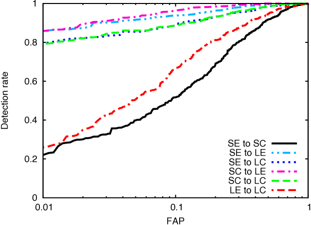
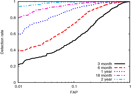
It is clear from Figure 2 that even using as little as 3 months of data, LISA can easily choose between the four models. With the exception of the SE/SC and LE/LC comparisons, each pair of models shows a detection rate in excess of at a false alarm rate. Models SE and SC are most difficult to distinguish with a detection rate of only at a false alarm rate, followed by models LE and LC with a detection rate of at that FAP. This is to be expected, as these pairs of models have the same seed mass distribution and differ only in the accretion prescription, so the distribution of masses for the events are quite similar (this pessimistic conclusion would most likely change if we included spins in our model waveforms). In the other cases, the mass distributions are quite distinct so the accurate mass measurements that are possible with LISA allow discrimination of the models with only a handful of events. In the left panel of Figure 3 we consider the SE to SC comparison and detector scenario (ii) only and show how the ROC performance depends on the mission duration. We see that our ability to distinguish models increases rapidly with the duration of the observation. For a 1 year observation we can distinguish SE and SC with a rate of for an FAP of , which is comparable to what can be achieved using a 3 month observation for the other comparisons.
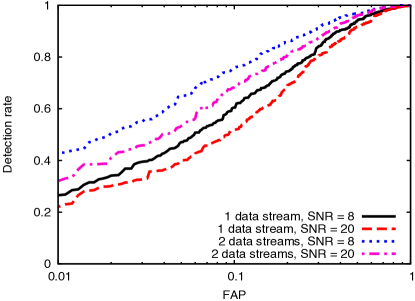
In the right panel of Figure 3 we again restrict to the SE to SC comparison, but now fix the observation to 3 months and show how the performance depends on the detector scenario. There is a relatively modest increase in performance for the more optimistic detector scenarios. At an FAP of , the detection rate increases from to going from the most pessimistic to the most optimistic scenario. The detector performance has a relatively weak effect since many of the events with the greatest distinguishing power have very high SNR and can be seen under any scenario. The use of two data streams rather than just one both increases the SNR of an event with given parameters and reduces the parameter estimation errors that arise due to instrumental noise. It is clear from Figure 3 that both of these are important, since both of the 2 data stream curves lies above both of the 1 data stream curves. If the SNR increase alone was important, we would expect the 2 data stream, SNR curve to lie between the one data stream curves, as SNR in two data streams corresponds to SNR in each data stream.
Reference [15] also studied MBHM model selection with LISA considering the same four models using the non-parametric Kolmogorov-Smirnov test to compare the distributions of one or two parameters between models. Their conclusions were broadly the same, i.e., that LISA can tell between models very easily. The approach described here has several advantages over theirs: we have a parametric model using the reasonable assumption of a Poisson distribution in each bin; we use the distribution of all model parameters simultaneously to compare models (3 in this case, but it is easily extendable to more); the present framework naturally extends to parameterised models for the underlying BH population, as used in the EMRI case; and, as described in Section 2, once actual LISA data is available, we will be able to fold the measured uncertainties in the source parameters into the analysis, rather than relying on theoretical estimates.
4 Discussion
We have described a framework for using the set of events observed by LISA to constrain models of the massive BH population in the Universe. Using EMRI events, we should be able to constrain the slope of a parametric model for the mass function of BHs in the LISA range to a precision of with just ten observed events and this improves with the number of observed events as . EMRI events alone will not be able to constrain any evolution of this mass function with redshift. LISA MBHM events can be used to choose between different models for the assembly of structure in the Universe. Assuming that the LISA events were drawn from one of four simple models, we have shown that we would be able to confidently identify the correct model after collecting as little as three months of LISA data. BHs in the LISA mass range, –, are not well constrained by current data, and so LISA has the potential to significantly improve our understanding of such systems and how they were assembled.
These preliminary results could be extended in several ways. The parameter space considered in the EMRI case should be expanded to explore what we can learn from EMRI measurements of BH spins and the eccentricities, inclinations etc. of EMRI orbits. MBHM waveform models including the merger/ringdown signal [27] and spin precession dynamics should improve our ability to distinguish between models. It will also be important to explore whether LISA EMRI and low- MBHM observations together can probe the redshift evolution of the mass function and break the degeneracy between the mass function and the mass-scaling of the EMRI rate.
In the MBHM model selection context, the four models considered were deliberately chosen in [6] to be as different as possible in order to provide ranges for the parameter estimation accuracies that might be achieved by LISA. It is therefore perhaps unsurprising that LISA will be able to distinguish these models very easily. The real Universe is likely to be a hybrid between light and heavy seed models, so it will be informative to explore more realistic mixtures between the present (oversimplified) seeding and accretion prescriptions. Indeed, if parameters can be introduced into the models that characterise the input physics (e.g., the seed mass distribution and accretion efficiency), we could determine the precision with which LISA will be able to measure such parameters. The results described here provide a clear illustration of the significant astrophysics that can be done with LISA observations and indicate that it will be worthwhile to carry out such more sophisticated analyses.
References
References
- [1] Volonteri M, Lodato G and Natarajan P 2008 MNRAS 383 1079–1088
- [2] Greene J E, Ho L C and Barth A J 2008 Astrophys. J. 688 159–179
- [3] Danzmann, K et al 1998 Lisa: Pre-phase a report, june 1998 Tech. rep. Garching, Germany
- [4] Sesana A, Volonteri M and Haardt F 2007 Mon. Not. Roy. Astron. Soc. 377 1711–1716
- [5] Gair J R 2009 Class. Quantum Grav. 26 094034–+
- [6] Arun K G, Babak S, Berti E, Cornish N, Cutler C, Gair J, Hughes S A, Iyer B R, Lang R N, Mandel I, Porter E K, Sathyaprakash B S, Sinha S, Sintes A M, Trias M, Van Den Broeck C and Volonteri M 2009 Classical and Quantum Gravity 26 094027–+
- [7] Barack L and Cutler C 2004 Phys. Rev. D 69 082005–+
- [8] Huerta E A and Gair J R 2009 Phys. Rev. D 79 084021–+
- [9] Greene J E and Ho L C 2007 Astrophys. J. 667 131–148
- [10] Sheth R K, Bernardi M, Schechter P L, Burles S, Eisenstein D J, Finkbeiner D P, Frieman J, Lupton R H, Schlegel D J, Subbarao M, Shimasaku K, Bahcall N A, Brinkmann J and Ivezić Ž 2003 Astrophys. J. 594 225–231
- [11] Gair J R, Tang C and Volonteri M 2010 Phys. Rev. D 81 104014–+
- [12] Volonteri M, Haardt F and Madau P 2003 Astrophys. J. 582 559–573
- [13] Begelman M C, Volonteri M and Rees M J 2006 Mon. Not. Roy. Astron. Soc. 370 289–298
- [14] Amaro-Seoane P, Gair J R, Freitag M, Miller M C, Mandel I, Cutler C J and Babak S 2007 Classical and Quantum Gravity 24 113–+
- [15] Plowman J E, Hellings R W and Tsuruta S 2010 ArXiv e-prints (Preprint 1009.0765)
- [16] Mackay D J C 2003 Information Theory, Inference and Learning Algorithms
- [17] Plowman J E, Jacobs D C, Hellings R W, Larson S L and Tsuruta S 2010 Mon. Not. Roy. Astron. Soc. 401 2706–2714
- [18] Wang Y, Holz D E and Munshi D 2002 Astrophys. J. Lett. 572 L15–L18
- [19] Berti E, Buonanno A and Will C M 2005 Class. Quant. Grav. 22 S943–S954
- [20] Hopman C 2009 Classical and Quantum Gravity 26 094028–+
- [21] Berti E and Volonteri M 2008 Astrophys. J. 684 822–828
- [22] Bardeen J M 1970 Nature 226 64–65
- [23] Thorne K S 1974 Astrophys. J. 191 507–520
- [24] Dotti M, Ruszkowski M, Paredi L, Colpi M, Volonteri M and Haardt F 2009 Mon. Not. Roy. Astron. Soc. 396 1640–1646
- [25] Dotti M, Volonteri M, Perego A, Colpi M, Ruszkowski M and Haardt F 2010 Mon. Not. Roy. Astron. Soc. 402 682–690
- [26] King A R and Pringle J E 2006 Mon. Not. Roy. Astron. Soc. 373 L90–L92
- [27] Berti E, Cardoso V and Will C M 2006 Phys. Rev. D 73 064030–+