Three-dimensional chemically homogeneous and bi-abundance photoionization models of the “super-metal-rich” planetary nebula NGC 6153

Abstract

Deep spectroscopy of the planetary nebula (PN) NGC 6153 shows that its heavy element abundances derived from optical recombination lines (ORLs) are ten times higher than those derived from collisionally excited lines (CELs), and points to the existence of H-deficient inclusions embedded in the diffuse nebula. In this study, we have constructed chemically homogeneous and bi-abundance three-dimensional photoionization models, using the Monte Carlo photoionization code mocassin. We attempt to reproduce the multi-waveband spectroscopic and imaging observations of NGC 6153, and investigate the nature and origin of the postulated H-deficient inclusions, as well as their impacts on the empirical nebular analyses assuming a uniform chemical composition. Our results show that chemically homogeneous models yield small electron temperature fluctuations and fail to reproduce the strengths of ORLs from C, N, O and Ne ions. In contrast, bi-abundance models incorporating a small amount of metal-rich inclusions ($\sim 1.3$ per cent of the total nebular mass) are able to match all the observations within the measurement uncertainties. The metal-rich clumps, cooled down to a very low temperature ($\sim 800$ K) by ionic infrared fine-structure lines, dominate the emission of heavy element ORLs, but contribute almost nil to the emission of most CELs. We find that the abundances of C, N, O and Ne derived empirically from CELs, assuming a uniform chemical composition, are about 30 per cent lower than the corresponding average values of the whole nebula, including the contribution from the H-deficient inclusions. Ironically, in the presence of H-deficient inclusions, the traditional standard analysis of the optical helium recombination lines, assuming a chemically homogeneous nebula, overestimates the helium abundance by 40 per cent.

1 Introduction

A long-standing dichotomy in nebular astrophysics is that the heavy element abundances derived from optical recombination lines (ORLs) are systematically higher than those derived from collisionally excited lines (CELs; see Peimbert & Peimbert 2006 and Liu 2006 for recent reviews). Temperature fluctuations (Peimbert 1967), density inhomogeneities (Rubin 1989; Viegas & Clegg 1994) and X-ray irradiation of quasineutral chemically homogeneous clumps (Ercolano 2009) have been proposed to explain this discrepancy. However, extensive observations of planetary nebulae (PNe) have shown that they are incapable of accounting for all observational features (Liu 2006). In order to explain the CEL/ORL abundance dichotomy, Liu et al. (2000, L2000 hereafter) presented a bi-abundance model. The model assumed that the nebula contains two gas components of different abundances — the diffuse component of “normal” composition that dominates the emission of CELs and another consisting of cold H-deficient inclusions posited in the diffuse gas that dominates the emission of ORLs. The model explains well spectroscopic observations from the ultraviolet (UV) to the infrared (IR). However, detailed photoionization models are still required to test this scenario and address issues such as: ‘How can the nebular physical conditions and its elemental abundances be reliably determined in the exiseence of chemical inhomogeneities?’, and ‘What is the nature and origin of the H-deficient clumps?’ To address these issues, this paper presents the results of three-dimensional photoionization modelling for the PN NGC 6153.

NGC 6153 is an archetypal nebula showing a particularly large ORL versus CEL abundance discrepancy factor (adf) of about ten (L2000). A large number of ORLs from a variety of heavy-element ions have been detected in this PN. NGC 6153 is thus an ideal object to model and to investigate the possible causes of the CEL/ORL abundance discrepancy problem. Early optical studies by Pottasch et al. (1984, 1986) suggested that NGC 6153 has a very high metallicity. The result was further corroborated by the observations of the Short Wavelength Spectrometer on board the Infrared Space Observatory (ISO-SWS) in the mid-IR ( Pottasch et al. 2003). L2000 presented a comprehensive spectroscopic analysis of NGC 6153 from the UV to the far-IR and found that the C, N, O, and Ne abundances derived from ORLs are about ten times higher than those derived from CELs. Using simple empirical models, L2000 showed that the discrepancy can be explained by assuming the existence of a H-deficient component embedded in the diffuse gas. Using optical integral field spectroscopic observations of three PNe including NGC 6153 with the Very Large Telescope Fibre Large Array Multi Element Spectrograph Argus integral field unit, Tsamis et al. (2008) provided further evidence for the existence of cold H-deficient inclusions and constrained their physical sizes to be smaller than $\sim$1,000 astronomical units. Péquignot et al. (2002, 2003) constructed one-dimensional photoionization models that contain two gas components of different abundances. The models reproduced satisfactorily most of the observed spectral features of NGC 6153. It is however difficult to self-consistently treat the diffuse radiation fields in one-dimensional models and investigate the size and spatial distribution of the postulated H-deficient clumps. This motivated us to carry out further modelling using the Monte Carlo photoionization code mocassin (Ercolano et al. 2003a, 2005, 2008) capable of dealing with an arbitrary nebular geometry and density and abundance distributions.

The paper is organized as follows. In Section 2, previous modelling work and observational data used to constrain our models are summarized. In Section 3, we introduce the code used for the modelling and present the modelling results. In Section 4, we discuss the implications and limitation of our results, the properties of the H-deficient inclusions and their impacts on nebular studies. A summary is given in Section 5.

2 Observations and previous models

In this section, we summarize observations available to constrain the photoionization models of NGC 6153 and introduce the earlier one-dimensional bi-abundance work of Péquignot et al. (2002, 2003), which serves as the starting point of our new three-dimensional models.

2.1 Spectroscopic observations

Spectra of NGC 6153 from the UV to the far-IR are available from the literature (e.g., L2000, Pottasch et al. 1984, 1986, 2003). For a given wavelength range, there may exist more than one set of observations. Due to varying aperture sizes, orientations and measurement uncertainties, different studies often obtain different fluxes for a given emission line. For the current work, we have adopted line fluxes of L2000, who present measurements in the optical obtained with ground-based facilities, in the UV obtained with the International Ultraviolet Explorer (IUE; 1150–3300Å), and in the mid- to far IR obtained with the Infrared Astronomical Satellite (IRAS;7.6–22.7 $\mu$m) and the Long Wavelength Spectrometer on board the ISO (ISO-LWS; 43–197 $\mu$m). L2000 obtained two sets of optical spectra. The set of spectra with the slit oriented along the nebular minor axis allows one to investigate the spatial brightness distribution of a given line along the slit. The other set, obtained by scanning the slit across the whole nebular surface, when combined with the total H$\beta$ flux [$\log$ $F$(H$\beta$) = $-$10.86 ergs cm^-2s^-1; Cahn et al. 1992], yields integrated fluxes of the whole nebula for all the detected lines. The integrated line fluxes can be directly compared with the model predictions. Note that L2000 used a logarithmic extinction, c(H$\beta$) = 1.30, deduced from the Balmer decrement, and the Galactic reddening law of Howarth (1983) to deredden the UV, optical and near-IR spectra. They adopted a different value c(H$\beta$) = 1.19, deduced from the observed radio continuum flux density and the H$\beta$ flux, to deredden the mid- and far-IR spectra. The same dereddening algorithm has been used in the current study. Here we have added a few mid-IR CELs falling within the spectral window of the ISO-SWS in our modelling. Given the fact that the size of the ISO-SWS diaphragm was not large enough to cover the entire nebula and the telescope pointing was offset by $3\aas@@fstack{\prime\prime}49$ east and $9\aas@@fstack{\prime\prime}0$ south of the nebular centre, aperture corrections have been applied by comparing the line fluxes obtained with ISO-SWS and those with IRAS. All strong emission lines considered in the previous modelling (L2000, Péquignot et al. 2003) were included in the current work, c.f. the next section for details.

In addition to line fluxes from the literature, we have supplemented the data with new observations using the B&C spectrograph mounted on the European Southern Observatory (ESO) 1.52 m telescope. The spectra, obtained on 2001 May 12, were taken in order to measure several near-IR emission lines (He i $\lambda$10830, [C i] $\lambda$9850, and [S iii] $\lambda$$\lambda$9069,9531), important for model constraints. The He i $\lambda$10830 line is particularly important to constrain the helium abundance in a bi-abundance model (c.f. Section 4.1). The spectra covered the wavelength range 7700–13254 Å, with the slit placed along the nebular minor axis. Two long exposures, each of 1800 s, and one short exposure of 300 s were made. The spectra were reduced using the long92 package in midas following the standard procedures. The spectra were bias-subtracted, flat-fielded, cosmic rays cleaned and wavelength-calibrated using exposures of a He-Ar calibration lamp. They were then flux-calibrated with the iraf package using wide-slit observations of HST standard stars. After dereddening, the spectra were normalized such that H i I(P12)/I(H$\beta$) = 0.01106, as predicted by the recombination theory, Case B (Storey & Hummer 1995) for ${\it T}_{\rm e}$ = 6,080 K and ${\it N}_{\rm e}$ = 3,500 cm^-3. The ${\it T}_{\rm e}$ and ${\it N}_{\rm e}$ values here are taken from L2000. Fluxes deduced from these observations are tabulated in Table 1 (see Section 3).

In an attempt to detect directly the postulated H-deficient knots and to constrain their physical sizes, we have also carried out long-slit spectroscopy of NGC 6153 using the STIS instrument on board the Hubble Space Telescope (HST). On 2002 June 3–4, two gratings, G430M and G750M, were used to cover the spectral range $\lambda$$\lambda$3050-5600 and $\lambda$$\lambda$5450-10100, respectively. A long slit of $52\arcsec\times 0\aas@@fstack{\prime\prime}2$ was placed along the nebular minor axis through the central star to cover the brightest parts of the nebula. The spatial resolution along the slit was $0\aas@@fstack{\prime\prime}05$/pixel. The standard pipeline procedures in iraf/stsdas were used to reduce the data. Unfortunately, these data suffered from poor signal-to-noise ratio as well as severe contamination by cosmic rays and turned out to be of very limited value for the current investigation (see Section 4.4).

Table 1: Comparison of the model predictions and the observations. The observed intensities have been dereddened and normalized such that $I$(H$\beta$)$=100$. Columns (4)–(12) give the ratios of predicted over observed values (departure ratios).

Line	$\lambda$ (Å)a	$I_{\rm obs}$	S	E1	E2	Bn	Bc	B	B${}^{\prime}_{\rm n}$	B${}^{\prime}_{\rm c}$	B′
H, He recombination lines, optical and radio continua
H$\beta$	4861.3	100	1.01	1.01	1.00	0.95	0.06	1.01	0.94	0.06	1.00
H$\alpha$	6562.8	298.08	0.97	0.97	0.97	0.90	0.08	0.98	0.90	0.08	0.98
H$\gamma$	4340.5	48.92	0.95	0.95	0.95	0.89	0.06	0.95	0.89	0.06	0.95
He i	3888.6	11.88	1.10	1.07	1.06	0.78	0.17	0.95	0.78	0.17	0.95
He i	4471.5	6.47	1.02	1.02	1.02	0.68	0.27	0.95	0.68	0.27	0.95
He i	5875.7	18.85	1.01	1.02	1.02	0.67	0.35	1.02	0.68	0.34	1.02
He i	6678.2	4.83	1.08	1.09	1.09	0.72	0.40	1.12	0.72	0.39	1.11
He i	7065.2	4.35	1.23	1.37	1.34	0.86	0.11	0.97	0.86	0.11	0.97
He i	7281.6	0.56	1.89	1.91	1.91	1.32	0.23	1.55	1.32	0.23	1.55
He i	10830.3	59.96	1.59	1.79	1.74	1.21	0.10	1.31	1.21	0.10	1.31
He ii	1640.0	82.19	1.03	0.98	0.99	0.86	0.13	0.99	0.81	0.21	1.02
He ii	4686.0	12.85	1.02	0.97	0.98	0.84	0.13	0.97	0.80	0.21	1.01
BJ/H$\beta$	3646	0.60	0.8	0.8	0.8	0.75	0.26	1.01	0.75	0.26	1.01
Heavy-element recombination lines
C ii	4267.2	2.42	0.16	0.16	0.16	0.10	0.85	0.95	0.10	0.82	0.92
C iii	4650+(M1)	0.50	1.11	0.76	0.76	0.41	0.27	0.68	0.40	0.39	0.79
C iii	4187(M18)	0.08	1.45	1.00	1.00	0.54	1.1	1.64	0.52	1.60	2.12
N ii	4041.3	0.24	0.19	0.21	0.21	0.15	0.89	1.04	0.16	0.84	1.00
N ii	4241.8	0.22	0.14	0.15	0.15	0.11	0.66	0.77	0.11	0.62	0.73
N ii	5679.0+(V3)	0.94	0.26	0.29	0.28	0.21	0.72	0.93	0.21	0.69	0.90
N iii	4379.0+(M17)	0.66	0.60	0.45	0.46	0.30	0.94	1.24	0.30	1.35	1.65
O ii	4075.0+(V10)	4.12	0.15	0.15	0.16	0.10	0.64	0.74	0.10	0.67	0.77
O ii	4089.3	0.55	0.13	0.13	0.14	0.09	0.83	0.92	0.09	0.86	0.95
O ii	4649.1	1.39	0.23	0.23	0.24	0.16	0.89	1.05	0.16	0.92	1.08
O ii	4651.0+(V1)	3.68	0.21	0.21	0.23	0.15	0.84	0.99	0.15	0.87	1.02
Ne ii	3340.0+(V2)	1.96	0.09	0.09	0.09	0.08	0.56	0.64	0.08	0.61	0.69
Ne ii	3700.0+(V1)	1.07	0.10	0.09	0.10	0.08	0.54	0.62	0.08	0.60	0.68
Ne ii	4392.0	0.15	0.11	0.11	0.11	0.06	0.56	0.65	0.09	0.61	0.70
Mg ii	4481.0	0.05				0.66	0.26	0.92	0.67	0.27	0.93
Collisionally excited lines (UV and optical)
[C i]	9850.3	0.17	0.06	0.17	0.34	0.25	0.07	0.32	0.26	0.05	0.31
C iii]	1907.0+	46.48	1.22	1.28	1.06	0.90	0.07	0.97	0.87	0.11	0.98
C iv	1549.0+	$<$30.0	1.08	0.61	0.61	0.53	0.00	0.53	0.49	0.00	0.49
[N i]	5199.0+	0.24	0.02	0.05	1.06	1.16	0.06	1.22	1.12	0.04	1.16
[N ii]	5754.6	0.83	0.30	0.61	0.75	1.03	0.21	1.24	1.08	0.20	1.28
[N ii]	6583.5+	64.20	0.31	0.72	0.99	1.08	0.05	1.13	1.11	0.05	1.16
N iii]	1744.0+	16.30	0.32	0.44	0.33	0.42	0.00	0.42	0.40	0.00	0.40
[O i]	6300.3	0.78	0.00	0.02	0.74	0.64	0.00	0.64	0.69	0.00	0.69
[O ii]	3726.1	18.9	0.40	0.75	0.89	0.86	0.22	1.08	0.90	0.25	1.15
[O ii]	3728.8	9.69	0.47	0.80	0.91	0.94	0.20	1.14	0.97	0.22	1.18
[O iii]	4363.2	4.19	0.90	1.05	0.93	0.92	0.00	0.92	0.88	0.01	0.89
[O iii]	5006.8+	1189.90	1.10	1.19	1.16	0.96	0.00	0.96	0.94	0.00	0.94
[Ne iii]	3869.0	93.91	0.96	1.00	0.95	1.01	0.00	1.01	0.99	0.00	0.99
[S ii]	4068.6	1.03	0.13	0.31	0.52	0.56	0.00	0.56	0.59	0.00	0.59
[S ii]	4076.4	0.35	0.13	0.31	0.52	0.55	0.00	0.55	0.58	0.00	0.58
[S ii]	6716.4	3.16	0.22	0.38	0.57	0.65	0.00	0.65	0.65	0.00	0.65
[S ii]	6730.8	5.26	0.19	0.36	0.56	0.61	0.00	0.61	0.62	0.62	0.62
[S iii]	6312.1	1.29	0.97	1.33	1.16	1.39	0.00	1.39	1.38	0.00	1.38
[S iii]	9068.9	39.74	0.86	1.10	1.03	1.09	0.00	1.09	1.09	1.09	1.09
[S iii]	9531.0	113.68	0.74	0.95	0.89	0.95	0.00	0.95	0.95	0.00	0.95
[Cl iii]	5517.7	0.55	1.07	1.13	1.01	1.08	0.00	1.08	1.07	0.00	1.07
[Cl iii]	5537.7	0.70	0.88	1.01	0.90	0.95	0.00	0.95	0.94	0.00	0.94
[Ar iii]	5191.8	0.10	0.83	0.84	0.77	0.94	0.00	0.94	0.91	0.00	0.91
[Ar iii]	7135.8	19.00	1.00	0.96	0.97	1.01	0.00	1.01	1.00	0.00	1.00
[Ar iv]	4711.4	2.54	1.00	0.97	0.98	0.95	0.00	0.95	0.93	0.00	0.93
[Ar iv]	4740.2	2.35	1.00	0.99	0.99	0.96	0.00	0.96	0.93	0.00	0.93
Collisionally excited lines (IR)
[N iii]	57.3 $\mu$m	72.43	1.14	1.03	1.02	0.85	0.16	1.01	0.86	0.16	1.02
[O iii]	51.8 $\mu$m	267.60	0.91	0.79	0.85	0.62	0.23	0.85	0.63	0.25	0.88
[O iii]	88.4 $\mu$m	74.44	0.84	0.60	0.65	0.49	0.13	0.62	0.49	0.14	0.63

Table 1: –continued

Line	$\lambda$ (Å)a	$I_{\rm obs}$	S	E1	E2	Bn	Bc	B	B${}^{\prime}_{\rm n}$	B${}^{\prime}_{\rm c}$	B′
[O iv]	25.9 $\mu$m	118.10	1.18	1.18	1.29	1.10	0.16	1.26	1.04	0.29	1.33
[Ne ii]	12.8 $\mu$m	23.14	0.07	0.11	0.15	0.16	1.00	1.16	0.15	0.68	0.83
[Ne iii]	15.6 $\mu$m	253.50	1.00	0.94	1.00	0.88	0.50	1.38	0.88	0.59	1.47
[Ne iii]	36.0 $\mu$m	32.61	0.65	0.60	0.64	0.57	0.18	0.75	0.57	0.21	0.78
[S iii]	18.7 $\mu$m	47.28	1.03	1.20	1.18	1.18	0.03	1.21	1.18	0.03	1.21
[S iii]	33.5 $\mu$m	32.61	0.81	0.78	0.77	0.80	0.02	0.82	0.80	0.01	0.81
[S iv]	10.5 $\mu$m	362.16	1.09	0.94	0.93	0.87	0.01	0.88	0.87	0.01	0.88
[Ar iii]	9.0 $\mu$m	56.34	0.40	0.37	0.39	0.37	0.01	0.38	0.37	0.01	0.38
[Ar iii]	21.8 $\mu$m	2.69	0.53	0.48	0.51	0.49	0.00	0.49	0.49	0.00	0.49

^a

‘+’ refers to the total intensity of the multiplet.

2.2 Imaging observations

Imaging observations of NGC 6153 have been carried out with ground-based telescopes (Pottasch et al. 1986) and the HST (L2000). Fig. 1 shows the HST images taken under programme GO-8594 (PI Liu) with the WFPC2 camera in the F502N and F656N narrow-band filters on 2000 August 13. Two 600s and two 500s exposures were made in the F502N and F656N filters, respectively. The pixel size was $0\aas@@fstack{\prime\prime}0455$. The images were co-added, cosmic-rays removed and calibrated following the standard recipes (e.g. Holtzmann et al. 1995). They were then dereddened using an extinction coefficient $c({\rm H}\beta)=1.30$. The two filters trace respectively emission of the [O iii] $\lambda$5007 and H$\alpha$ lines, although there could be some contamination from the nebular continuum emission and the [N ii] $\lambda$$\lambda$6584,6548 lines in the case of F656N. We performed aperture photometry and found that H$\alpha$ and [O iii] $\lambda$5007 line fluxes deduced from HST images agreed within 10 per cent with the corresponding values yielded by the optical scanning spectrum of L2000, suggesting insignificant contamination to the HST F656N image from the [N ii] lines and the nebular continuum emission.

The azimuthally averaged radial surface brightness distribution of H$\alpha$ was deduced from the HST F656N image and plotted in Fig. 2. The profile is used in our models to constrain the nebular density distribution.

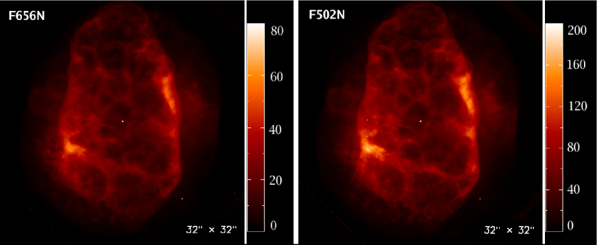
Figure 1: HST/WFPC2 images of NGC 6153 obtained with the F656N (left panel) and F502N (right panel) narrow-band filters. North is up and east to the left. The units of the color bars are $10^{-13}~{}{\rm ergs~{}cm}^{-2}~{}{\rm s}^{-1}~{}{\rm arcsec}^{-2}$.

2.3 Previous models

Previous empirical and one-dimensional photoionization models of NGC 6153 provide valuable insight and a useful guide for setting the initial parameters of the new 3D photoionization models. L2000 constructed several parametrized empirical models to match the observed fluxes of selected ORLs and CELs. Recombination contributions to CELs were considered. They obtained the following results: 1) Models of a uniform chemical composition and density distribution cannot reproduce the large strengths of ORLs; 2) Chemically homogeneous models with density variations predict too weak ORLs and the hydrogen Balmer discontinuity and a too strong [Ne iii] fine-structure line compared to observations; and 3) Bi-abundance models consisting of two components, each with a different temperature, density, and chemical composition, can account for most of the observed patterns of NGC 6153. Two different bi-abundance models were presented by L2000. One assumed some low-density (${\it N}_{\rm e}$ = 700 cm^-3) and low-temperature (${\it T}_{\rm e}$ = 500 K) H-deficient material embedded in the “normal” nebular gas of ${\it N}_{\rm e}$ = 5,500 cm^-3 and ${\it T}_{\rm e}$ = 9,500 K. In the other model, the hydrogen-depleted material was assumed to be fully ionized and have a high density ($2\times 10^{6}$ cm^-3) and a moderate temperature of 4,700 K. In both models, the helium and heavy element abundances with respect to hydrogen in the H-deficient component were respectively $~{}4$ and$~{}100$ times higher than the corresponding values in the diffuse gas.

Péquignot et al. (2002, 2003) constructed detailed bi-abundance photoionization models of NGC 6153 using the one-dimensional code NEBU. Their models were composed of sectors extracted from a number of spherically symmetric models, each made of different input parameters except the central ionizing source. In the models, a H-deficient component with a small filling factor was mixed with a normal-composition shell. They found that models containing a small amount of dense, cold H-deficient material [$M$ = 0.0031$\mathrm{{\it M}_{\odot}}$, ${\it N}({\rm H})$ = 4 410 cm^-3, ${\it T}_{\rm e}$ = 1 390 K] in pressure equilibrium with the surrounding gas of “normal” composition [$M$ = 0.38$\mathrm{{\it M}_{\odot}}$, ${\it N}{\rm(H)}$ = 1 170 cm^-3, ${\it T}_{\rm e}$ = 9 040 K] can well account for the observed fluxes of most ORLs and CELs. Compared to the normal gas, the H-deficient component is enhanced in helium and CNONe elements by factors of 6 and 100, respectively. Nevertheless, the average elemental abundances of the entire nebula are only slightly affected by the presence of the H-deficient component, given its small mass. Péquignot et al. (2002) pointed out that helium abundance relative to hydrogen will be overestimated if composition fluctuations are not taken into account and it is also essential to consider collisional contribution to excitation of He i lines to correctly determine helium abundance.

3 Models

The modelling is carried out using mocassin (Version 2.02.12; Ercolano et al. 2003a, 2005), a fully three-dimensional Monte Carlo photoionization code that solves the radiative transfer self-consistently in an iterative way and is designed to tackle problems involving density variations and chemical inhomogeneities. The code is therefore suitable for the current investigation aiming to study the effects of the complicated geometry and possible chemical inhomogeneities of NGC 6153. To reduce degree of freedom, the ionizing star is assumed to have a blackbody spectral energy distribution in our models. A more realistic representation of the ionizing star is left to a later work. The nebula is approximated by a cubical Cartesian grid of cells of individually pre-defined density and chemical composition. For each cell, the radiation fields (including the stellar and the diffuse component) and physical conditions (electron temperature, density and ionic fractions of all elements considered) are calculated iteratively. Based on an initial guess of the temperature and ionization structures, the code calculates radiation fields, solves the ionization and thermal equilibrium equations and then updates the temperature and ionization structures. This process is iterated until physical conditions are converged in most cells. Finally, the emission spectrum of the model nebula is calculated by integrating over the volume of the nebula. The code has been applied to construct photoionization models of the PN NGC 3918, the H-deficient knots in the “born-again” PN Abell 30, the Wolf-Rayet PN NGC 1501 (Ercolano et al. 2003b,c, 2004) and PN NGC 6781 (Schwarz & Monteiro, 2006).

In our models, we have assumed that NGC 6153 has an azimuthally symmetrical structure in the x and y plane and a reflection symmetry in Z and placed the central star at the centre of a corner cell of a $48\times 48\times 48$ cubic grid. Modelling in this way can effectively save the computational time since only one eighth of the nebula is simulated. The HST images of NGC 6153 show that the nebula can be approximated by an ellipsoidal shell with enhanced emission in the equator. The brightest part of the nebula exhibits point symmetry with respect to the central star, probably implying the existence of an ellipsoidal ring lying along the major axis in the south-east to the north-west direction. A faint halo can also be seen surrounding the bright nebula. In order to better constrain the input parameters, we have constructed a series of models with progressively increasing complexity. These include a spherical model (model S), two ellipsoidal models without and with a torus (models E1 and E2, respectively), and a bi-abundance model (model B). The spherical and ellipsoidal models are chemically homogeneous. Table 2 gives the adopted model parameters that yield the best match to the observations. In Table 1, we compare the predicted line fluxes with the observations. Further details of our models are presented below.

Table 2: Model parameters.

Parameter	S	E1	E2	Bn	Bc	B
L (e36 ergs s-1)	16	14	14	13	13	13
${\it T}_{\rm eff}$ (kK)	90	92	92	92	92	92
M (M⊙)	0.349	0.269	0.267	0.243	0.0031	0.246
${\it N}_{\rm tot}$(H) (e56)	2.63	2.03	2.02	2.07	0.0081	2.08
He	0.138	0.138	0.138	0.10	0.50	0.102
C (e$-$4)	5.4	4.9	4.9	3.2	177	3.88
N (e$-$4)	4.6	4.6	4.6	3.8	150	4.37
O (e$-$4)	6.82	6.82	7.44	5.63	440	7.33
Ne (e$-$4)	1.87	1.76	1.90	1.76	177	2.44
Mg (e$-$5)				3.8	12.1	3.83
Si (e$-$5)				3.5	11.3	3.53
S (e$-$5)	1.75	1.75	1.75	1.75	5.16	1.76
Cl (e$-$7)	3.0	2.56	2.53	2.35	10.1	2.38
Ar (e$-$6)	3.0	2.75	3.0	2.9	11.5	2.93
Fe (e$-$6)				1.5	110	1.92
$\tau_{\rm x}$a (H i)	2.61	8.91	362.6			473
$\tau_{\rm z}$b (H i)	2.63	3.69	5.275			6.1
$\tau_{\rm x}$c (He i)	0.54	1.83	73.72			95.7
$\tau_{\rm z}$d (He i)	0.54	0.76	1.088			1.24
$\tau_{\rm x}$e (He ii)	74.5	89.1	120.5			90.1
$\tau_{\rm z}$f (He ii)	77.6	53.7	59.93			42.1
$\langle$${\it T}_{\rm e}$$\rangle$ (K)	8,663	8,825	8,583	9,007	815	8,892
$t^{2}$g	0.008	0.006	0.006			0.014

3.1 Updates to mocassin

For the purpose of our study, we have made a number of updates to mocassin Version 2.02.12, including incorporation of He i line emissivities valid at low temperatures, di-electronic recombination of the third-row elements of the periodic table, recombination contributions to CELs, and photoionization depopulation of the He i meta-stable level 2 ³S.

3.1.1 He i  line emissivities

The original code uses He i  line emissivities at one electron density of 10² cm^-3 for ${\it T}_{\rm e}$ range 5,000–20,000 K, insufficient to treat emission from the cold component ($T_{\rm e}\la 1,000~{}\rm{K}$) present in our bi-abundance model. In addition, emissivities of some He i lines, such as the $\lambda$10830, are sensitive to electron density. Using the calculations of Benjamin et al. (1999) and Smits (1996), we have extended the He i  line emissivities in the code to cover the density range 10²–10⁶ cm^-3 and the temperature range 312.5–5,000 K. Note that emissivities of a few weak He i lines ($\lambda$2946, $\lambda$3615, $\lambda$4122, $\lambda$4439, $\lambda$5049, and $\lambda$9466) for this low temperature range are unavailable. Collisional excitation from the He i 2 ³S and 2 ¹S meta-stable levels is insignificant at low temperatures, and is only considered for ${\it T}_{\rm e}$  $>$ 5,000 K. Using the atomic data of Porter et al. (2005), Porter et al. (2007) have provided the most recent He i  line emissivities. Aver et al. (2010) have compared the results of Porter et al. (2007) and Benjamin et al. (1999). The differences therein are generally small compared to the “departure ratios” in Table 1.

3.1.2 Radiative transfer of He i

For the He i singlets, Case B recombination is assumed. For the He i triplets, the lowest term, 2 ³S, is meta-stable and thus considerably populated, leading to significant self-absorption and collisional excitation from this level. The He i 2s ³S – 3p ³P $\lambda$3888 line suffers the strongest suppression due to self-absorption. A fraction of those photons, depending on the optical depth, are absorbed and converted into the $\lambda$7065 line photons. The He i $\lambda$10830 line is strongly affected by collisional excitation. In fact, it is mainly excited by the collisional process He i 2s ³S – 2p ³P. Thus, an accurate calculation of the population of level 2s ³S is essential to predict reliable fluxes of the He i $\lambda$$\lambda$3888,7065,10830 lines. The 2s ³S level is populated by recombinations of He⁺ with electrons to He⁰ triplet levels, and is depopulated by the following processes (Clegg and Harrington 1989): (a) collisional excitation to He⁰ singlet levels; (b) radiative decay to the ground state; (c) collisional ionization by thermal electron impacts; (d) photoionization by UV photons with $\lambda\la$ 2600 Å, such as the resonant H i Ly$\alpha$ photons; (e) decay from the He i 2p ³P state to the ground state following collisional excitation and the trapping of $\lambda$10830 photons in the nebula. Among these processes, (e) contributes only a few per cent of the destruction of 2s ³S and thus can be neglected. Processes (a)–(c) have been considered by Benjamin et al. (1999) but not process (d), because its effects depend on the surrounding radiation fields that are unknown without detailed modelling. The original mocassin code does not consider the destruction of meta-stable helium by the photoionization of trapped resonant H i Ly$\alpha$ photons, a process that has been shown to be important for compact and optically-thick PNe (Clegg & Harrington 1989). This process is introduced in our updated version. With the He i 2s ³S level population determined, the self-absorption of the He i $\lambda$3888 line can be treated using a Monte Carlo approach. Following the absorption of a He i $\lambda$3888 photon from the 2s ³S state to 3p ³P state, it can either scatter back or cascade down through the 3s ³S and 2p ³P states with a probability about 0.9 and 0.1, respectively. In the latter case, three photons ($\lambda$4.3 $\mu$m, $\lambda$$\lambda$7065,10830) are emitted. The self-absorption problem of He i triplets has been investigated by Robbins (1968) by solving an integral equation of transfer for the ideal case of a uniform sphere expanding with a constant velocity gradient. For this ideal case, the results deduced from our Monte Carlo approach agree within 10 per cent with those of Robbins for $\tau(\lambda 3888)$ $\la 10$.

3.1.3 Di-electronic recombination of S, Cl and Ar

While no reliable di-electronic recombination rates for the third-row elements have been published to date, they are estimated to be larger than or at least comparable in magnitude to their radiative counterparts. Considering the fact that the rates seem to follow a certain trend with ionization stage, Ali et al. (1991) suggested that for a given ion Xⁱ⁺, better estimates of the di-electronic recombination rates than zero can be obtained by taking the average of the rates for the second-row elements Cⁱ⁺, Nⁱ⁺, Oⁱ⁺. Dudziak et al. (2000) adopted coefficients empirically calibrated with an unpublished model of the PN NGC 7027. More recently, Ercolano et al. (2004) obtained upper limits to the rate coefficients of S²⁺, Cl²⁺ and Ar²⁺ by modelling the PN NGC 1501. In our modelling, we have assumed that the di-electronic recombination rates of S, Cl and Ar are all proportional to those of O, and determined their actual values by optimizing the model fit to observations (see Section 4.1).

3.1.4 Recombination contributions to CELs

Radiative cascades following recombination (radiative and di-electronic) of heavy element ions can partially contribute to the emission of CELs, especially for lines from the meta-stable levels of low-ionization ions. This process is included when calculating the emissivities of CELs from [C i], [C iii], [N i], [N ii], [N iv], [O ii], [O iii], [Ne iv] and [Ne v]. Here the relevant radiative and di-electronic recombination rates are taken from Péquignot et al. (1991) and Nussbaumer and Storey (1984), respectively, except [N ii] and [O ii], for which the total recombination rates calculated by P. J. Storey (private communication) are used.

3.1.5 Convergence criteria

mocassin uses the Monte Carlo method to simulate the propagation of photons inside a nebula. Thus, one of the key component of the code is its convergence criteria. The original convergence indicator used in the code is the neutral hydrogen fraction, namely a model is deemed as converged if the fraction of neutral hydrogen in most cells varies less than 5 per cent for two adjacent iterations. However, only using the fraction of neutral hydrogen as convergence criteria cannot guarantee the convergence for other ions, especially for cells in the Xⁱ⁺/X^(i-1)+ transition regions. For example, we find that in a “converged” model based on the original criterion, the integrated He²⁺/He ratio may vary 10 per cent after additional iterations. To overcome this, we have also expanded the convergence criteria to include integrated intensities of emission lines from helium and heavy element ions, such as the He ii $\lambda 4686$ and [O iv] 25.9 $\mu$m, in our modelling.

3.2 Central star

The properties of the central star are basic input parameters in the models. Based on the detection of broad O vi $\lambda$3811 and C iv $\lambda$5801 features, L2000 classified the central star of NGC 6153 as a [WC]-PG 1159 H-deficient star. The classification is supported by a study of the UV spectrum of the central star (Pottasch et al. 2003). Using the blackbody approximation, we have calculated the effective temperature (${\it T}_{\rm eff}$), luminosity, core mass, and surface gravity of the central star using the Zanstra method (Zanstra 1931) and the Stoy method (Stoy 1933). The results are listed in Table 3. In the calculations, we have assumed the distance to NGC 6153 to be 1.5 kpc (Péquignot et al. 2003). Both the Zanstra and Stoy methods require a measurement of the stellar continuum flux of the central star. For this purpose we have made use of the HST/WFPC2 F502N image and find a stellar continuum flux of $2.75\times 10^{-14}$ ergs cm^-2 s^-1 Å^-1 at 5 010 Å after subtracting the nebular background emission. The applicability of the Zanstra method also requires the nebula to be optically thick, which is probably not the case for the H i Lyman continuum given that NGC 6153 is a high-excitation class PN and is probably matter bound. Thus the Zanstra temperature deduced from the H$\beta$ flux gives only a lower limit, while that deduced from the He ii $\lambda$4686 line is closer to the actual value since the nebula is likely to be optically thick in the He ii Lyman continuum. The Stoy method has the advantage that it does not depend on the nebular optical depth. However, the applicability of this method requires the measurement of the total flux of all cooling lines from the UV to the far-IR, not an easily achievable task. We find that the Stoy temperature is lower than the He ii Zanstra temperature, suggesting that the total flux of the nebular cooling emission lines might have been underestimated.

Table 3: Parameters of the central star.

	${\it T}_{\rm eff}$	$L$	${\it M}_{\rm core}$	$\log g$
	(${\rm K}$)	(${\rm L}_{\odot}$)	(${\rm M}_{\odot}$)	(${\rm{cm~{}s^{-2}}}$)
Stoy method	76,530	2,034	0.562	5.37
H i Zanstra method	76,260	2,014	0.562	5.37
He ii Zanstra method	90,090	3,228	0.586	5.47

3.3 Spherical model

3.3.1 Model parameters

An initially chemically homogeneous spherical model (referred as model S hereafter) is constructed. Its density distribution is constrained by the azimuthally averaged radial surface brightness distribution of H$\alpha$ deduced from the HST/WFPC2 F656N image. We find that a density distribution given by

$$\rho_{s}(r,\theta,\Phi)=N_{0}(s{\times}f(r|a_{1},b_{1})+(1-s){\times}f(r|a_{2},b_{2}))$$ (1)

where

$$f(r|a,b)=\frac{1}{4\pi b^{a}\Gamma(a)}r^{a-3}\exp(-r/b)$$ (2)

can reasonably reproduce the observed H$\alpha$ surface brightness distribution, as shown in Fig. 2. The parameters are: $a_{1}=23$, $b_{1}=0.0118$, $a_{2}=12$, $b_{2}=0.037$, and $s=0.2$. Note that the shell is actually composed of two density profiles with peaks at $r~{}=~{}(a_{1,2}-3)\times b_{1,2}$ and FWHMs $(a_{1,2}-3)/b_{1,2}$, as illustrated in Fig. 3. In Eqs (1) and (2), $r$ ranges from 0 to 0.5, corresponding to a nebular angular radius of $0\arcsec$ to $16\arcsec$. A black body spectral energy distribution for the ionized source is assumed. The model was constructed taking the ${\it T}_{\rm eff}$ and luminosity of the central star, the nebular elemental abundances and the total mass as free parameters.

Figure 2: Comparison between the observed (dashed line) and model-predicted (solid line) azimuthally averaged radial surface brightness distribution of H$\alpha$ of model S.

Figure 3: Radial number density distribution of hydrogen atoms N(H) of the spherical model (solid line). It is composed of two components with different profiles (dashed lines).

3.3.2 Model results

The spherical model has a total mass of 0.35 M_⊙ and is fully ionized by the central star which has a ${\it T}_{\rm eff}$  of 90,000 K and a luminosity of 4,000 L_⊙. The nebula is optically thin in both the H i and He i ionizing continua, but is optically thick in the He ii ionizing continuum. The electron temperature throughout the nebula is remarkably uniform. We obtain a mean electron temperature of 8,663 K, lower than the value derived from the [O iii] temperature diagnostic lines, and a small mean-square temperature fluctuation parameter $t^{2}$ (as defined by Peimbert 1967) of 0.008.

Fig. 4 shows the radial temperature and density distributions and the ionization structures of the spherical model. In Fig. 4 (also in Figs. 7 and particularly 13), the sharp temperature dip in the high-ionization region ($r\sim 3-4\arcsec$) is due to efficient cooling by the strong [Ne v]  fine-structure lines at 24.2 $\mu$m and 14.3 $\mu$m. This feature, which is a consequence of the low (but not zero) density assumed close to the star in the present model, has negligible effect on the model nebular emission. The decline of temperature for $r$ between $4\arcsec$ and $8\arcsec$ is caused by the enhanced cooling of the [O iii] lines, as the ionic concentration of O²⁺ increases with $r$.

The predicted over observed line flux ratios (hereafter ’departure ratios’) are given in the 4th column of Table 1. Most hydrogen and helium recombination lines are well matched by the model. The small remaining discrepancies between observed and predicted fluxes are within observational uncertainties, except for the He i $\lambda$$\lambda$7281,10830 lines. The latter two lines with large departure ratios will be further discussed in Section 4. The model however fails to explain the strengths of all heavy element ORLs where the model predictions are generally about one order of magnitude lower than the observed values.

The fluxes of CELs from high-ionization species are reasonably reproduced by the model. For low-ionization species, such as [C i], [N i], [O i], [O ii] and [S ii], the predicted fluxes are significantly lower than observed. This can be ascribed to the oversimplified density distribution assumed in the spherical model. The nebula is clearly ellipsoidal and bipolar, and appears to be ionization-bound at least in some directions, where low-ionization species can survive. We infer that there exists a dense torus and present two ellipsoidal models without and with a torus in the next subsection.

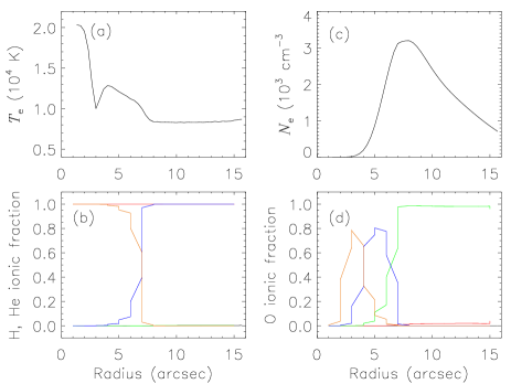
Figure 4: Distributions of ${\it T}_{\rm e}$ (panel a); ${\it N}_{\rm e}$ (panel c); H, He (panel b) and O (panel d) ionization structures of the spherical model. In panel b, the yellow, blue, green, red, and black lines represent those of He²⁺, He⁺, He⁰, H⁺ and H⁰, respectively. In panel d, the yellow, blue, green, red, and black lines represent those of O⁴⁺, O³⁺, O²⁺, O⁺ and O⁰, respectively.

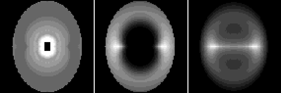
Figure 5: Distributions of ${\it T}_{\rm e}$  (left panel), N(H) (middle panel) and the surface brightness of H$\alpha$ (right panel) in the x-z plane for model E1. The contours are of arbitrary units.

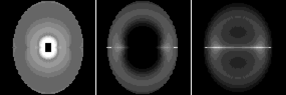
Figure 6: Distributions of ${\it T}_{\rm e}$  (left panel), N(H) (middle panel) and the surface brightness of H$\alpha$ (right panel) in the x-z plane for model E2. The contours are of arbitrary units.

3.4 Ellipsoidal models

3.4.1 Model parameters

To investigate possible effects of the geometry, we have built two ellipsoidal models without (model E1) and with (model E2) a torus. Based on the HST images, we assume that the nebula has a semimajor axis of 16$\arcsec$ in the polar (z-) direction and a semiminor axis of 12$\arcsec$ in the equatorial (x- and y-) plane. The density distribution of the ellipsoid is set by

$$\rho_{e}(r,\theta,\Phi)=\frac{\rho_{s}(\frac{r}{1+c|\cos(\theta)|})}{1+d|\cos(\theta)|^{g}},$$ (3)

where $\rho_{s}$ was defined in Eq (1). For the ellipsoidal models, the parameters $a$, $b$, and $s$ are set to the same values as those adopted in model S. We introduce three new parameters $c$, $d$, and $g$ to characterize the density gradient in the equatorial plane and the polar direction. The values of $c$, $d$, and $g$ are constrained by the HST images as well as the observed fluxes of low- and high- excitation CELs. Via model fitting, we obtain $(c,d,g)=(1,0.8,0.5)$ for model E1 and $(0.8,0.5,0.5)$ for model E2. A torus with a width of 6 cells and a height of 1 cell is added in model E2. Its density is assumed to be 2.5 times higher than the original values of the replaced cells. The density distributions of model E1 and model E2 in the x-z plane are displayed in the middle panels of Figs. 5 and 6, respectively.

3.4.2 Model results

Figs. 5 and 6 display the distributions of the predicted temperature, hydrogen number density and the surface brightness of H$\alpha$ of models E1 and E2, respectively. Fig. 7 shows the model radial distributions of the electron temperature, density and ionization structures. In Fig. 8, we compare the predicted line fluxes of model E2 with observations. We find that both models E1 and E2 give a better fit to the [N ii], [O ii], and [S ii]  lines compared to model S thanks to the density enhancement in the equatorial plane. Model E2 yields a better fit for the [C i] and [N i]  lines than model E1, owing to the presence of a dense torus. For the remaining lines, models E1 and E2 give similar results of model S. Although the ellipsoidal models show improvements in reproducing CELs from low-ionization ions, like model S, they fail to reproduce the strengths of heavy element ORLs, strongly indicating that chemical inhomogeneities have to be invoked.

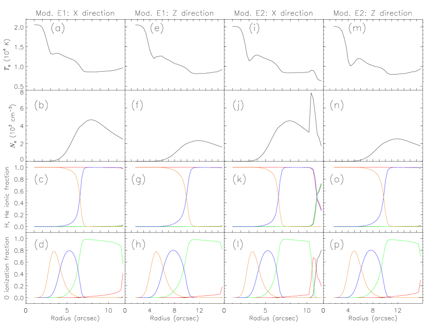
Figure 7: ${\it T}_{\rm e}$ and ${\it N}_{\rm e}$  distributions and H, He and O ionization structures in the two ellipsoidal models. Panels (a) – (d) and (e) – (h) are for the x, z directions in the ellipsoidal model E1, respectively; Panels (i) – (l) and (m) – (p) are for the x, z directions in the ellipsoidal model E2, respectively. In panels (c), (g), (k), and (o), the yellow, blue, green, red and black lines represent the fractions of He²⁺, He⁺, He⁰, H⁺ and H⁰, respectively. In panels (d), (h), (l), and (p), the yellow, blue, green, red, and black lines represent the fractions of O⁴⁺, O³⁺, O²⁺, O⁺ and O⁰, respectively. Note that the sharp features near 10$\aas@@fstack{\prime\prime}$5 in panels (i), (j), (k) and (l) are produced by the dense torus.

Figure 8: Comparison of line fluxes predicted by model E2 and observations for ORLs (left panel) and CELs (right panel).

3.5 Bi-abundance model

3.5.1 Model parameters

For the bi-abundance model, we assume that there are some metal-rich knots (cells) embedded in the diffuse nebula of “normal” abundances. The density distribution of the diffuse nebula is inherited from model E2, but with a slightly reduced mass. The spatial distribution of the metal-rich cells is set randomly by the probability density function $f(r|a_{3},b_{3})$ (see Eq (2)), where $r$ ranges from 0 to 0.3125 (i.e. 0–10″), $a_{3}=22$ and $b_{3}=0.013$, as constrained by the surface brightness distribution of the O ii $\lambda$4649 ORL along the nebular minor axis (see Fig. 19 of L2000). In Fig. 9, we compare the profile of the predicted O ii  surface brightness with observations. In the comparison, we have included the effects of seeing and convolved the predicted surface brightness distribution with a Gaussian function of FWHM $3\aas@@fstack{\prime\prime}2$. Positions of individual knots are set by Monte Carlo simulations. Their three-dimensional spatial distribution is illustrated in Fig. 10. Fig. 11 shows the distributions of number density of knots and of the hydrogen atoms of the diffuse gas. In order to reduce the random uncertainties, we have generated four samples of knots. Line fluxes yielded by the four samples are in good agreement (within 10 per cent). They are then averaged to compare with the observations. The model parameters are given in Table 2, where B_n and B_c represent respectively components of “normal” composition and of cold metal-rich knots, and B is the sum of the two components. Note that for the normal component, we have fixed the helium abundance to 0.1 (as adopted by Péquignot et al. 2003). As pointed out by Péquignot et al., observations of helium recombination lines in the optical alone are not sufficient to decompose the helium abundance in the two components. For the H-deficient knots, the element abundances heavier than neon are assumed to be the corresponding solar values in mass, considering that PNe originate from low- and intermediate- mass stars that can not process the third-row elements.

Figure 9: Comparison of the measured surface brightness distribution (“+”) of the O ii $\lambda$4649 ORL and the model prediction (solid line).

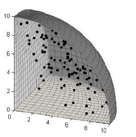
Figure 10: Three-dimensional spatial distribution of metal-rich knots (cells) in the bi-abundance model. The units of the axes are arcsec.

Figure 11: Radial distribution of the volume number density of metal-rich knots given by the analytic (solid line) and Monte Carlo simulations (asterisks). The dashed and dash-dotted lines represent the density distribution of hydrogen atoms in the diffuse nebular gas along the x and x axes, respectively.

3.5.2 Model results

Fig. 12 displays the predicted structure of ${\it T}_{\rm e}$ and ${\it N}_{\rm e}$. The radial distributions of temperature, density and the ionization structures in four directions across the four metal-rich knots marked in Fig. 12 are shown in Fig. 13. An inspection of the two figures shows that the knots have been cooled down to very low temperatures ($\sim 800$ K), and create shadows that block the ionizing UV radiation field from the central star, leaving low ionization regions behind them. As in models S, E1 and E2, there is a temperature dip at $r\sim 3-5\arcsec$. Fig. 14 displays the predicted monochromatic images of H$\beta$, [O iii] $\lambda$5007, and O ii $\lambda$4649. The figure clearly shows that the [O iii] CEL originates from the “normal” component, while the O ii ORL is dominated by knots. In spite of their small number, metal-rich knots have a non-negligible contribution to H$\beta$ emission, owing to the enhanced emissivity at low temperatures and high densities. In Fig. 15, we compare the predicted line fluxes with the observations, demonstrating that the bi-abundance model has significant improvements in reproducing the strengths of heavy element ORLs and the hydrogen Balmer discontinuity. In addition, the model yields a much better fit to the measured flux of the [Ne ii] 12.8 $\mu$m line, which is underestimated by all the chemically homogeneous models. This is due to the fact that the metal-rich knots are enriched in Ne and have a large Ne⁺ ionic concentration.

Model B generally supports the results of the one-dimensional models of Péquignot et al. (2002, 2003) in terms of properties of the H-deficient inclusions such as the electron temperature, density, mass and chemical abundances. Those values in model B (${\it T}_{\rm e}$ = 1,390 K, ${\it N}({\rm H})$ = 4,410 cm^-3, $M$ = 0.0031$\mathrm{{\it M}_{\odot}}$ and oxygen enrichment factor of about 100) are comparable to those given by the one-dimensional models (${\it T}_{\rm e}$ = 815 K, ${\it N}({\rm H})$ = 4,000 cm^-3, $M$ = 0.0031$\mathrm{{\it M}_{\odot}}$ and oxygen enrichment factor of about 80). Beyond constraining the properties of the H-deficient inclusions in a self-consistent manner, the three-dimensional model enables to investigate sizes and spatial distributions of the H-deficient inclusions which one-dimensional models can not. Detailed line by line comparison between model B and the one-dimensional models by Péquignot et al. (2002, 2003) is not easy, due to different geometric configurations, density structures, spectral energy distributions of the ionizing star and atomic data used. We do not claim superiority of predicted fluxes of model B over the one-dimensional models. To understand how three-dimensional bi-abundance models advance the field of modelling of emission line gaseous nebulae, simple bi-abundance benchmark models are needed. Then the comparison between three-dimensional model results and one-dimensional model results will be much easier to carry out and interpret, but this is beyond the scope of the current paper.

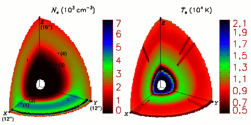
Figure 12: Predicted ${\it N}_{\rm e}$(left panel) and ${\it T}_{\rm e}$ (right panel) distributions in the bi-abundance model B.

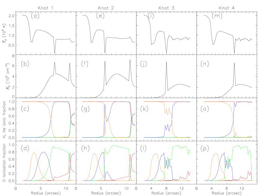
Figure 13: Distributions of ${\it T}_{\rm e}$, ${\it N}_{\rm e}$  and H, He and O ionization structures along a radial direction that passes through the marked four knots in Fig. 12. Panels (a) – (d) and (e) – (h) are for the Knots 1 and 2 located in the xy plane, respectively; Panels (i) – (l) and (m) – (p) are for the Knots 3 and 4 in the yz plane, respectively. In panels (c), (g), (k) and (o), the yellow, blue, green, red, and black lines represent the fractions of He²⁺, He⁺, He⁰, H⁺ and H⁰, respectively. In panels (d), (h), (l) and (p), the yellow, blue, green, red, and black lines represent the fractions of O⁴⁺, O³⁺, O²⁺, O⁺ and O⁰, respectively. Note that in panels (b) and (f), the peaks at $\sim 8\arcsec$ and $\sim 11\arcsec$ correspond respectively to the knot and the torus.

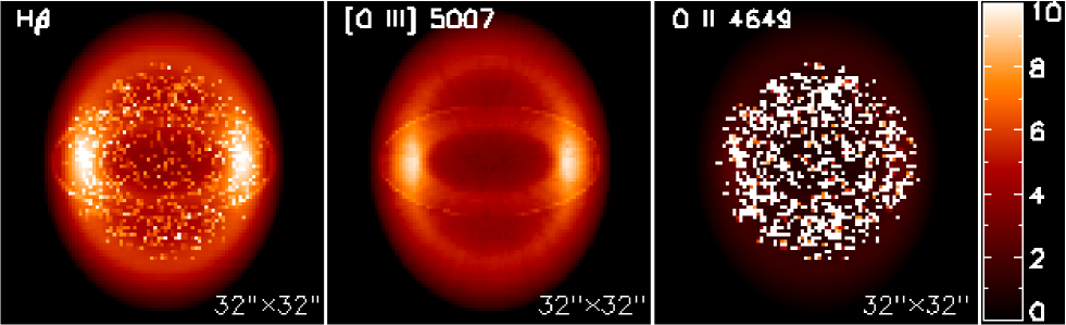
Figure 14: Projected monochromatic images of H$\beta$ (left panel), [O iii] $\lambda$5007 (central panel) and O ii $\lambda$4649 (right panel) predicted by the bi-abundance model B at a viewing angel of $\theta$ = 60 deg. $\theta$ = 0 deg is for face on. The units of the color bars are $10^{-13},10^{-12}~{}{\rm and}~{}10^{-15}~{}{\rm ergs}~{}{\rm cm}^{-2}~{}{\rm s}^{-1}~{}{\rm arcsec}^{-2}$ for the three images, respectively.

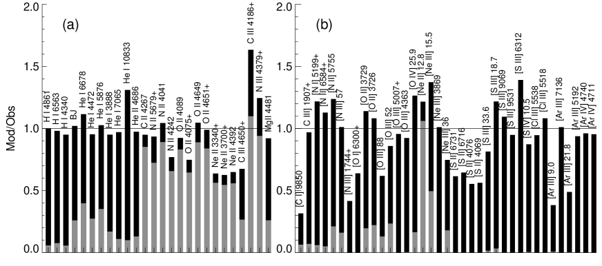
Figure 15: Comparison of the predicted and observed line fluxes for ORLs (left panel) and CELs (right panel) in the bi-abundance model B. Black and gray parts represent contributions from the normal and the cold H-deficient components, respectively.

4 Discussion of the bi-abundance model

4.1 Uncertainties and discrepancies

Uncertainties in our models include errors in the atomic data, in the treatment of the radiation transfer and uncertainties in the adopted line fluxes. The estimates of the di-electronic recombination rates ($\alpha_{d}$) for S, Cl and Ar are rather rough. We have assumed that $\alpha_{d}$(S, Cl, Ar) = $\eta$(S, Cl, Ar) $\times$ $\alpha_{d}$(O), where the constants $\eta$(S, Cl, Ar) are obtained by fitting the observations. Only two [Cl iii]  lines are detected, insufficient to place a constraint on the $\eta$(Cl) value. We have thus assumed $\eta$(Cl) $=1$. S and Ar have a number of lines detected from several ionization stages. We obtain $\eta$(S, Ar) = (0.76, 6.8), (0.45, 4.0), (0.35, 4.0) and (0.35, 4.0) from the models S, E1, E2 and B, respectively. In the bi-abundance model, the di-electronic recombination coefficients of S and Ar are respectively 0.32 and 14 times the corresponding radiative recombination values. Our estimates of $\alpha_{d}$(S, Ar) differ from those obtained from the modelling of NGC 7027 (Dudziak et al. 2000) by a factor of three. On the other hand, these uncertainties in the di-electronic recombination rates of S and Ar are unlikely to have a large impact on our model predictions for other lines, considering the low abundance of Ar and the fact that [S ii], [S iii] and [S iv] lines have similar emissivities, and consequently thermal structure is hardly affected by the uncertainties in the ionization structure of S.

The bi-abundance model underestimates the flux of C iii multiplet M1, but overestimates that of M18. This is probably caused by errors in the atomic data. The existing calculations of the radiative (Péquignot et al. 1991) and di-electronic (Nussbaumer & Storey 1984) recombination coefficients for C iii may not be applicable to plasma at very low temperatures. Further theoretical work is urgently needed to study the behavior of recombination lines in extremely cold plasma. We note that because of a larger di-electronic contribution the emissivity of lines from C iii multiplet M18 is much more sensitive to electron temperature than that of M1. Should it not be the case, the model would have yielded a much better fit to both M1 and M18.

The bi-abundance model overestimates the flux of the He i $\lambda$10830 line by 21 per cent. The He i $\lambda$10830 line is crucial for the bi-abundance model in that, unlike other He i  lines, it is predominantly collisionally excited, and thus has the potential to constrain the helium abundance in the hot component of “normal” composition. Its usage is however hindered by the complexity in the He i 2s³S meta-stable level population and the excitation and radiative transfer of the He i $\lambda$10830 line. Observations of several PNe have shown that the measured He i line ratio I($\lambda$10830)/I($\lambda$5876) is lower than the theoretical prediction (see, e.g., Peimbert & Torres-Peimbert 1987a,b). Possible explanations include the destruction of He i $\lambda$10830 photons by internal dust (Kingdon & Ferland 1995), and the photoionization depopulation of the He i meta-stable level by H i Ly$\alpha$ photons (Clegg & Harrington 1989). The later process has been considered in our model. However its inclusion reduces the predicted flux of the He i $\lambda$10830 line only slightly. Additional destruction mechanisms may be needed to reconcile observations with theory.

Given its high sensitivity to electron temperature, the He i $\lambda$7281 line serves as an important diagnostic to probe the physical conditions in the cold H-deficient knots (Zhang et al. 2005a). Although improved compared to the chemically homogeneous models, our bi-abundance model overestimates the He i $\lambda$7281 line by 55 per cent. The discrepancy is probably caused by departure from the Case B assumption. Under Case A recombination, the predicted flux of the He i $\lambda$7281 line is about a factor of two lower. L2000 and Liu et al. (2001) find that the observed fluxes of the 2s¹S-np¹P and 2p¹P-ns¹S series are systematically lower than predicted by Case B recombination. Similar discrepancies are also found in H ii regions, such as the Orion Nebula (Porter et al. 2007; Blagrave et al. 2007) and 30 Doradus (Tsamis & Péquignot 2005). Porter et al. (2007) pointed out that although the escaping of the He i Lyman photons could cause the discrepancies, it is not consistent with the fact that the He i $\lambda$6678 line flux is not decreased compared to prediction. We also want to point out that in the case of the escaping He i Lyman photons, the discrepancy factors for the np¹P-2s¹S series ($n=3,4,5$) will decrease with increasing $n$ values, which is also not seen in the Orion Nebula. In their non-Case-B, self-consistent “model III”, Porter et al. (2007) attributed the discrepancies to “inaccurate reddening corrections”. Another plausible mechanism is that He i Lyman photons are absorbed by hydrogen atoms or dust grains, as proposed by Liu et al. (2001). We conclude that while Case B recombination may still remain a good approximation for the He i singlet lines in some PNe (e.g. NGC 7027; Zhang et al. 2005b), significant departures from this approximation may occur in others, and the effects can be quite significant for the 2s¹S-np¹P and 2p¹P-ns¹S series.

We deduce the extinction coefficient $c({\rm H}\beta)$ by comparing the observed H i and He ii  line ratios to theoretical values, assuming a constant electron temperature and density. In the presence of a cold, H-deficient component, such as in the bi-abundance model, the extinction coefficient thus derived would be overestimated, leading to the fluxes of lines of short wavelengths being systematically overestimated while those of long wavelengths underestimated. This effect is nevertheless small, less than 5 per cent in the current bi-abundance model.

4.2 ${\it T}_{\rm e}$  fluctuations versus the bi-abundance model

${\it T}_{\rm e}$ fluctuations have been proposed to explain the CEL/ORL abundance discrepancies as well as the differences between the electron temperatures derived from the [O iii] CELs and from the hydrogen Balmer discontinuity (e.g. Peimbert & Peimbert, 2006). However, chemically homogeneous models predict a very small $t^{2}$. Using the formula of Peimbert (1967) and the values of $T_{\rm e}$([O iii]) and $T_{\rm e}$([H i]) measured by L2000, we find $t^{2}=0.065$, much larger than the values predicted by chemically homogeneous models ($t^{2}\leq 0.008$; Table 2). The bi-abundance model yields a larger value ($t^{2}\simeq 0.014$), but still significantly lower than the 0.065 derived from the measured $T_{\rm e}$([O iii]) and $T_{\rm e}$([H i]). Note that the formalism of Peimbert (1967) is only applicable to situations of small amplitudes of temperature variations. It will significantly overestimate $t^{2}$ in the case where the nebula is composed of two distinct components of very different temperatures (Zhang et al. 2007). By satisfactorily reproducing observations of the [O iii] CELs and the hydrogen Balmer discontinuity, the bi-abundance model provides a natural explanation for the discrepancy between $T_{\rm e}$([O iii]) and $T_{\rm e}$([H i]).

4.3 Properties of the cold component

Table 4 summarizes the properties of the H-deficient knots derived from the bi-abundance model. The model shows that the knots are fully ionized and optically thin, with ${\it T}_{\rm e}$  of 800 K, a hydrogen number density of 4,000 cm^-3, a He/H abundance ratio of 0.5, and CNONe abundances relative to hydrogen about 40–100 times higher than the “normal” component. The mass of this cold H-deficient component is only 0.0031 M_⊙ ($\sim 3$ Jupiter masses), about 1 per cent of the total mass of the nebula.

With much enhanced metal abundances compared to the “normal” component, the cooling of the cold component is dominated by the IR fine-structure lines from C, N, O and Ne ions. These fine-structure lines have different excitation temperatures, typically much lower than those of optical/UV CELs. Their emissivities are thus less sensitive to temperature than optical/UV CELs. These IR lines also have relatively low, yet varying critical densities. Therefore, depending on the local physical conditions, their contributions to the cooling vary. It follows that the electron density plays an important role in setting the equilibrium temperatures of the cold component by determining which IR lines are dominant coolants. At low electron densities, the [O iii] 52 and 88 $\mu$m lines are the dominant coolants, whereas at higher densities, the [Ne ii] 12.8 $\mu$m and [Ne iii] 15.6, 36 $\mu$m lines, owing to their higher critical densities and higher excitation temperatures than the [O iii] lines, start to dominate the cooling. Because the [Ne ii]  and [Ne iii]  IR lines have higher excitation temperatures than the [O iii] IR lines, the equilibrium temperatures in high-density knots are higher than those in low-density ones. For example, as hydrogen number density decreases from 10,000 cm^-3 to 1,000 cm^-3, the equilibrium temperature drops from 1,070 K to 460 K. It follows that both the density and temperature contrasts between the cold component and the normal component are expected to grow as the nebula expands, assuming that the two components are in pressure equilibrium. As a consequence, one expects the adf value to increase as the nebula evolves, consistent with what is observed (e.g. Zhang et al. 2004). The equilibrium temperatures in the H-deficient knots are also affected by the He and heavy element abundances in that the photoionization of He dominates the heating whereas the CNONe IR lines control the cooling. We find that an increase of 60 per cent in He abundance or a decrease of 20 per cent in CNONe abundances leads to an increase of 200 K in the equilibrium temperature. It should be mentioned that, because of the lack of suitable diagnostic tools, densities of the H-deficient inclusions are not well constrained in the current models. This introduces some uncertainties in the estimate of the total mass of the cold component. It is also worth pointing out that in the bi-abundance model, electron temperatures deduced from ratios of IR CELs to optical CELs, such as the [Ne iii] 15.6 $\mu$m/$\lambda$3869 ratio, are expected to be lower than the value derived from the [O iii] optical line ratio, consistent with the observations (e.g. Bernard-Salas et al. 2004).

We compare the pressures of the cold inclusions and their surrounding gas in Fig. 16. On average, the two components have a pressure ratio $P({\rm cold})/P({\rm normal})=0.53\pm 0.77$, which means that the H-deficient knots have a large range of pressure relative to the surrounding gas. This departure from pressure equilibrium could be a consequence of some simplifying assumptions of the model. In the model we assume that the H-deficient knots have the same hydrogen number density, and the main nebula has a smoothly varying density distribution except the equatorial torus. However, the departure is not deleterious to our conclusions.

The H-deficient knots are thermally stable. If the electron temperature increases, the enhanced thermal pressure will force the knots to expand and thus decrease the density, leading to enhanced cooling that will reduce the temperature. This property may help survival of H-deficient knots during the PN evolution phase.

Figure 16: Pressure ratios of cold H-deficient knots and their surrounding gas in the bi-abundance model.

In the current bi-abundance model, the cold H-deficient knots are distributed in the nebular inner region (within 10 arcsec) in order to reproduce the ORL surface brightness distributions yielded by long-slit observations (L2000). It seems to be a common characteristic of PNe that ORL strengths peak at the nebular centre, e.g., PN NGC 7009 (Luo et al. 2001; Tsamis et al. 2008), PN NGC 6720 (Garnett & Dinerstein 2001). Our modelling also shows that in order to match the strength of the [Ne ii]  12.8 $\mu$m line, which originates mainly from the cold component, the knots must be located relatively close to the central star in order to avoid over-production of Ne⁺ ions. It is unclear whether this concentration of H-deficient inclusions near the nebular centre is a consequence of their lower expansion velocity compared to the main diffuse gas or whether they form from a later evolutionary phase of the central star.

Given their high densities, high CNONe abundances and low ionization degrees, the cold knots absorb hard ionizing photons more efficiently than the diffuse gas, and thus weaken and soften the stellar radiation fields passing through them. As a result, the radial shadow tails behind the H-deficient knots have lower temperatures and ionization degrees than their nearby “unshielded” gas. These effects are visible in Figs. 12 and 13. The presence of these shadow regions is however unlikely to have major effects on ORLs and low-ionization CELs or on $t^{2}$ values.

Finally, we point out that the current investigation of the properties of H-deficient inclusions can be much improved with better IR observations. Restricted by the computer memory, the knots are not spatially resolved at all in the current modelling. This rules out the possibility to study structure and properties of optically thick H-deficient knots as well as effects of knots smaller than the model resolution limit. In addition, the current work does not take into account the effects of dust grains, a potential heating source (e.g. Stasińska & Szczerba 2001). Given the different physical and chemical conditions, the dust grains in H-deficient knots presumably differ in properties from those in the “normal” gas. Future modelling that takes into account the effects of dust grains on nebular ionization and thermal structures may be worthwhile.

Table 4: Properties of the H-deficient inclusions in model B.

$\langle$${\it T}_{\rm e}$$\rangle$ (K)	815
$\langle$${\it N}_{\rm H}$$\rangle$ (cm-3)	4 000
$\langle$${\it N}_{\rm e}$$\rangle$ (cm-3)	6 680
M (M⊙)	0.0031
Mass fraction	1.3 %
Number of cells	872
Cell size	$0\aas@@fstack{\prime\prime}25\times 0\aas@@fstack{\prime\prime}25\times 0\aas@@fstack{\prime\prime}33$
Filling factor	0.002
He/H	0.50
C/H	0.01177
N/H	0.0150
O/H	0.0440
Ne/H	0.0177

4.4 Size of H-deficient knots

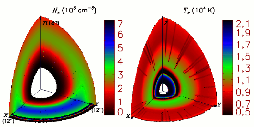
Figure 17: Three-dimensional structures of ${\it N}_{\rm e}$(left panel) and ${\it T}_{\rm e}$ (right panel) of model B^′ that used a higher spatial resolution of 96³ (see text).

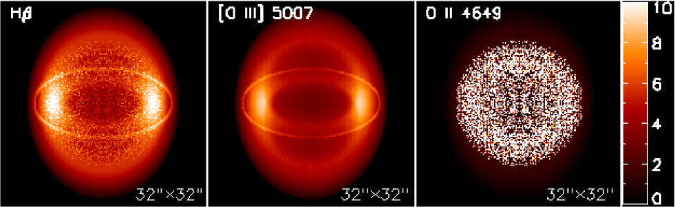
Figure 18: Projected monochromatic images of H$\beta$ (left panel), [O iii] $\lambda$5007 (central panel) and O ii $\lambda$4649 (right panel) of model B^′ at a viewing angel of $\theta$ = 60 deg. The units of the color bar are $10^{-13},10^{-12}$ and  $10^{-15}~{}{\rm ergs}~{}{\rm cm}^{-2}~{}{\rm s}^{-1}~{}{\rm arcsec}^{-2}$ for the three images, respectively.

The grainy H$\beta$ image predicted by model B (Fig.  14) is not consistent with the HST observation, suggesting that size of the postulated H-deficient inclusions must be smaller than adopted in this model. In order to investigate possible effects of assumed knot size on model results, we have constructed another bi-abundance model of higher resolution using a grid of 96³ cells (model B^′). For this new model, all the input parameters are the same as those used in model B except that the physical size of knots (cells) is reduced by half and the number of knots is increased by a factor of 8. Fig. 17 shows the electron density and temperature structures predicted by model B^′. The resultant ORL and CEL images are displayed in Fig. 18. The predicted total line fluxes as well as the contributions from the two components are presented in the last three columns of Table 1. For most lines, the differences between models B and B^′ are small. The cold H-deficient knots in model B^′ have slightly higher ionization degrees than those in model B due to their smaller physical size in model B^′. There are however significant differences between the two models for the ionic fractions of high-ionization ions such as C³⁺, N³⁺, O³⁺ and He²⁺ as well as low ionization ions such as Ne⁺. As a result, the predicted fluxes of lines from those ions vary dramatically. For example, the [Ne ii] 12.8 $\mu$m line flux emitted by the cold H-deficient knots in model B^′ decreases by 50 per cent compared to model B, while the fluxes of C iii, N iii ORLs emitted by the cold H-deficient knots increase by 50 per cent, and the fluxes of He ii lines and the [O iv] 25.9 $\mu$m line are almost doubled. These results imply that lines such as the [Ne ii] 12.8 $\mu$m CEL and C iii, N iii ORLs can potentially be used to constrain the size of the cold H-deficient inclusions. This is however complicated by the fact that intensities of these lines are also affected by the electron density in the cells as well as their spatial distribution.

In an attempt to better constrain the size of the cold knots, the STIS spectra obtained by us have been used to deduce the surface brightness distribution of the C ii $\lambda$4267 line, the strongest ORL detected by STIS. The spectra are unfortunately quite noisy and suffer from severe cosmic ray contamination. Nevertheless, we find the observed surface brightness distribution across the nebula is smoother than predicted by model B^′, suggesting that the postulated cold H-deficient inclusions must have sizes smaller than $1/6\arcsec$ (i.e. 250 AU at a distance of 1.5 kpc).

4.5 Elemental abundances

In Table 5, we list the chemical abundances of NGC 6153 derived from the bi-abundance model B and those in the literature obtained from traditional empirical analyses. For comparison, we also give the solar abundances presented by Asplund et al. (2009). Table 5 shows that the heavy element abundances deduced from optical/UV CELs, which are systematically lower than values yielded by infrared CELs (Pottasch et al. 2003), are in excellent agreement with those of the “normal” component; whereas the heavy element abundances deduced from infrared CELs are close to the average values of the whole nebula, and are much lower than the abundances in the cold component. The helium abundance published in the literature, deduced from the empirical method assuming a homogeneous composition, has been significantly overestimated due to the contamination of cold knots (see also Péquignot et al. 2002). If this is also the case for H ii regions, the primordial helium abundance deduced from the standard analyses of helium recombination lines of metal-poor galaxies will be overestimated. The He, C, N, O and Ne abundances in the cold knots are respectively 5, 55, 40, 80 and 100 times higher than those in the main nebula.

Table 5: Elemental abundances of NGC 6153.

Elem.	L2000a	P03b	Bn	Bc	B	Solarc
He	0.14	0.14	0.10	0.50	0.102	0.085
C($-$4)	2.8	6.8	3.2	177	3.88	2.692
N($-$4)	2.3	4.8	3.8	150	4.37	0.676
O($-$4)	5.0	8.3	5.63	440	7.33	4.898
Ne($-$4)	1.7	3.1	1.76	177	2.44	0.851
Mg($-$5)			3.8	12.1	3.83	3.981
Si($-$5)			3.5	11.3	3.53	3.236
S($-$5)	1.6	1.9	1.75	5.16	1.76	1.318
Cl($-$7)	4.2	5.6	2.35	10.1	2.38	3.162
Ar($-$6)	2.7	8.5	2.9	11.5	2.93	2.512

^a

from L2000 for optical/UV CELs.

^b

from Pottasch et al. (2003).

^c

from Asplund et al. (2009).

4.6 Possible origins of the postulated H-deficient inclusions

Given that adf values measured for PNe are always larger than unity, H-deficient inclusions are presumably a genuine feature of PNe. Their presence in PNe is however not predicted by current theories of stellar evolution. While it has been proposed (Iben et al. 1983) that an evolved star undergoing a very late helium flash (the so called “born-again” PNe) may harbor H-deficient material, the central stars of most PNe exhibiting large adf’s are found not to be H-deficient. Hydrogen-deficient knots have been clearly detected in the two “born-again” PNe, Abell 30 and Abell 58. On the other hand, Wesson et al. (2003, 2008) found that the H-deficient knots in Abell 30 and Abell 58 are oxygen-rich, in contrast to the expectation of the “born-again” scenario. Their chemical composition has more in common with neon novae than with Sakurai’s Object. The latter is believed to have recently experienced a final He-shell flash. Lau et al. (in preparation) explore the possibility of binary evolution to account for the observed high oxygen and neon abundances of the H-deficient knots in Abell 58, assuming that the knots are from the ejecta of a neon nova explosion. They consider a number of scenarios but none fit perfectly with the observations. Their best scenario consists of binary stars where the primary ONe white dwarf provided the neon nova explosion and the secondary asymptotic giant branch star evolved into the PN. This scenario requires very fine-tuned initial conditions, particularly the initial separation, to make the neon nova occur just after the final flash of the secondary asymptotic giant branch companion. Therefore, this scenario does not predict a large number of PNe with H-deficient knots.

Another conjecture is that the H-deficient inclusions are evaporating solid bodies, such as metal-rich planetesimals formed in planetary disks (Liu et al. 2006). This scenario has been subsequently investigated by Henney & Stasińska (2010), who show that the destruction of solid bodies during the short PN phase itself is not able to provide enough metal-rich material to explain the observed CEL/ORL abundance discrepancies, due to a low sputtering rate. On the other hand, the sublimation of solid bodies during the final stages of the asymptotic giant branch phase, which is much longer than the PN phase, might provide enough metal-rich material and serve as a possible mechanism causing the abundance discrepancies.

Although other explanations to the (moderate) ADF of HIIRs are still possible, the H-deficient inclusions may also be present in H ii regions (Tsamis et al. 2003; Tsamis & Péquignot, 2005). They could be supernovae ejecta in the form of metal-rich droplets that fall back into the interstellar medium after a long journey lasting about 10⁸ yr (Stasińska et al. 2007). They might also originate from evaporating proto-planetary disks around newly formed stars, such as the proplyds discovered in the Orion Nebula.

5 Summary

We have constructed detailed three-dimensional photoionization models of NGC 6153 of spherical or ellipsoidal geometry, with and without H-deficient inclusions. The model results are compared with spectroscopic observations from the UV, optical to the far IR as well as narrow-band imaging observations. In those models, the main nebula is assumed to be chemically homogeneous and of a “normal” composition. The spherical model can reproduce the strengths of hydrogen and helium recombination lines and of high excitation CELs. In order to explain the strengths of low-excitation CELs, we have considered an ellipsoidal shell where the density decreases from the equator to the poles, supplemented with an equatorial torus having the same chemical composition but of a higher density. The chemically homogeneous ellipsoidal model with a torus reproduces the strengths of all CELs within the measurement uncertainties, but fails by an order of magnitude for heavy element ORLs. In all cases, chemically homogeneous models yield small temperature fluctuations, and are therefore incapable to explain the large discrepancy between $T_{\rm e}({\rm[O~{}{\sc III}]})$ and $T_{\rm e}({\rm H~{}{\sc I}})$. In contrast, a bi-abundance model, incorporating small-scale chemical inhomogeneities in the form of a small amount of metal-rich inclusions, not only reproduces the strengths of heavy element ORLs and the hydrogen Balmer discontinuity, but also improves the overall fitting of CELs.

In our best-fit bi-abundance model, the CNONe abundances in the metal-rich knots are enhanced by 40–100 times compared to those of the main nebula. The presence of those metal-rich knots increases the average metal content of the whole nebula by 30 per cent. Optical/UV CELs arise mainly from the main diffuse nebula of “normal” composition and thus probe the physical conditions and chemical abundances of this component. IR CELs originate from both components, and thus yield elemental abundances higher than optical/UV CELs but lower than ORLs. In addition, temperatures deduced from IR CELs tend to be lower than values deduced from optical/UV CELs. For He i lines, although a large fraction of their fluxes arises from the H-deficient component, given the relatively low abundance enhancement factor of about 5, the helium abundance of the normal component remains a fair representation of the average value of the whole nebula. Nevertheless, in the presence of H-deficient inclusions, the traditional analysis assuming a single uniform chemical composition for the whole nebula, will greatly overestimate the helium abundances of the normal component. One should bear in mind that in the current work we were unable to separate helium emission originating from the two components to obtain reliable estimates of the helium abundance in each of the two components. Indeed, we have assumed He/H $=0.1$ for the normal component. The collisional excitation dominant He i $\lambda$ 10830 line can, in principle, be used to estimate the helium abundance in the normal component. Its usage is however hampered by observational and theoretical uncertainties. The electron temperature inside the metal-rich knots is as low as 800 K. The main coolants are IR fine-structure lines from heavy element ions, including the [O iii] 52, 88 $\mu$m, the [Ne iii] 15.6, 36 $\mu$m and [Ne ii] 12.8 $\mu$m lines. The metal-rich knots have a high density, and are roughly in pressure equilibrium with the surrounding “normal” gas. The metal-rich knots weaken and soften the UV radiation field. The cometary tails of “normal” gas behind the knots have relatively low temperatures and ionization degrees.

We show that the presence of metal-rich knots may lead to significant errors in nebular properties derived from the traditional methods assuming a single nebular component. We discuss physical and chemical properties of the metal-rich knots in NGC 6153 as well as their possible origins. To better constrain the nature of metal-rich knots in PNe, new observations and techniques are useful. For example, both imaging and spectroscopic observations of IR fine-structure lines at high spatial resolution and sensitivity will certainly shed new insight into the properties of these metal-rich knots. In future work, we plan to develop more comprehensive methods to probe these cold knots by involving more observational features (e.g. He I discontinuities; Zhang et al. 2005a, 2009) and up-to-date recombination coefficients of ORLs for low-temperature plasma (Fang et al. in preparation). We will also construct detailed three-dimensional models for more PNe exhibiting large adf’s with resolved metal-rich knots, such as M 1-42. These are the subjects of further papers.

Acknowledgments We would like to thank the referee for the valuable comments, which helped improve the quality of the paper. The modelling was carried out on the SGI Altix330 System at the Department of Astronomy at Peking University, HP supercomputer operated by the Center for Computational Science and Engineering at Peking University and the Columbia supercomputer operated by the NASA Advanced Supercomputing (NAS) Division at Ames Research Center. We acknowledge our awards, SMD-08-0633 and SMD-09-1154, of High-End Computing (HEC) time on NAS and NCCS resources by the NASA Science Mission Directorate (SMD). We thank Johnny Chang for his able and generous support of our research using Columbia. This research has made use of NASA’s Astrophysics Data System Bibliographic Services. BE is supported by an STFC Advanced Fellowship. YZ acknowledges financial support from the Seed Funding Programme for Basic Research in HKU (200909159007).

References

- [1] Ali B., Blum R. D., Bumgardener T. E., Cranmer S. R., Ferland G. J., Haefner R. L., Tiede G. P., 1991, PASP, 103, 1182
- [2] Asplund M., Grevesse N., Sauval A.J., Scott P., 2009, ARA&A, 47, 481
- [Aver et al.(2010)] Aver E., Olive K. A., Skillman E. D., 2010, JCAP, 5, 3
- [3] Benjamin R. A., Skillman E. D., Smits D. P., 1999, ApJ, 514, 307
- [4] Bernard-Salas J., Houck J. R., Morris P. W., Sloan G. C., Pottasch S. R., Barry D. J., 2004, ApJ, 154, 271
- [5] Blagrave K. P. M., Martin P. G., Rubin R. H., Dufour R. J., Baldwin J. A., Hester J. J., Walter D. K., 2007, ApJ, 655, 299
- [6] Cahn J. H., Kaler J. B., Stanghellini L., 1992, A&AS, 94, 399
- [7] Clegg R. E. S., Harrington J. P., 1989, MNRAS, 239, 869
- [8] Dudziak G., Péquignot D., Zijlstra A. A., Walsh J. R., 2000, A&A, 363, 717
- [Ercolano(2009)] Ercolano B. 2009, MNRAS,397, L69
- [Ercolano et al.(2003)] Ercolano B., Barlow M. J., Storey P. J., Liu X.-W., 2003a, MNRAS, 340, 1136
- [9] Ercolano B., Barlow M. J., Storey P. J., Liu X.-W., Rauch T., Werner K., 2003c, MNRAS, 344, 1145
- [Ercolano et al.(2005)] Ercolano B., Barlow M. J., Storey P. J. 2005, MNRAS, 362, 1038
- [10] Ercolano B., Barlow M. J., De Marco O., Rauch T., Liu X.-W., 2004, MNRAS, 354, 558
- [11] Ercolano B., Morisset C., Barlow M. J., Storey P. J., Liu X.-W., 2003b, MNRAS, 340, 1153
- [Ercolano et al.(2008)] Ercolano B., Young P. R., Drake J. J., Raymond J. C. 2008, ApJS, 175, 534
- [12] Fang X., Storey P. J., Liu X.-W., 2010, in prep
- [13] Ferland G. J., Korista K. T., Verner D. A., Ferguson J. W., Kingdon J. B., Verner E. M., 1998, PASP, 110, 761
- [Garnett & Dinerstein(2001)] Garnett D. R., Dinerstein H. L., 2001, ApJ, 558, 145
- [14] Henney W. J., Stasińska G., 2010, ApJ, 711, 881
- [15] Holtzmann J.A., Burrows C. J., Casertano S., et al., 1995, PASP, 107, 1065
- [16] Howarth I. D., 1983, MNRAS, 203, 301
- [Iben et al.(1983)] Iben I., Jr Kaler J. B., Truran J. W., Renzini A., 1983, ApJ, 264, 605
- [17] Kingdon J., Ferland G. J., 1995, ApJ, 403, 211
- [18] Lau H. B, de Marco O., Liu X.-W., 2010, in prep
- [\citeauthoryearLiu2006] Liu X.-W., 2006, in IAU Symp. 234 Planetary Nebulae, eds. Barlow M. J., Méndez R. H. (Cambridge: Cambridge University Press), P.219
- [19] Liu X.-W., Luo S.-G., Barlow M. J., Danziger I. J., Storey P. J., 2001, MNRAS, 327, 141
- [Liu et al.(2000)] Liu X.-W., Storey P. J., Barlow M. J., Danziger I. J., Cohen M., Bryce, M., 2000, MNRAS, 312, 585
- [20] Luo S.-G., Liu X.-W., Barlow M. J., 2001, MNRAS, 326,1049
- [21] Nussbaumer H., Storey P. J., 1984, A&AS, 56, 293
- [22] Peimbert M., 1967, ApJ, 150, 825
- [\citeauthoryearPeimbert & Peimbert2006] Peimbert M., Peimbert A., 2006, in IAU Symp. 234 Planetary Nebulae, eds. Barlow M. J., Méndez R. H. (Cambridge: Cambridge University Press), P.227
- [23] Peimbert M., Torres-Peimbert S., 1987a, Rev. Mex. Astr. Astrofis., 14, 540
- [24] Peimbert M., Torres-Peimbert S., 1987b, Rev. Mex. Astr. Astrofis., 15, 117
- [25] Péquignot D., Amara M., Liu X.-W., Barlow M. J., Storey P. J., Morisset C., Torres-Peimbert S., Peimbert M., 2002, RMxAC, 12, 142 ”Photoionization Models for Planetary Nebulae with Inhomogeneous Chemical Composition”
- [Péquignot et al.(2003)] Péquignot D., Liu X.-W., Barlow M. J., Storey P. J., Morisset C., 2003, in Planetary Nebulae: Their Evolution and Role in the Universe, IAU Symp. 209, Eds Kwok S., Dopita M., Sutherland R. (ASP), p. 347
- [26] Péquignot D., Petitjean P., Boisson C., 1991, A&A, 251, 680
- [27] Porter R. L., Ferland G. J., MacAdam K. B., 2007, ApJ, 657, 327
- [Porter et al.(2005)] Porter R. L., Bauman R. P., Ferland G. J., MacAdam K. B. 2005, ApJL, 622, L73
- [28] Pottasch S. R., Beintema D. A., Raimond E., et al., 1984, ApJ, 278, 33
- [29] Pottasch S. R., Bernard-Salas J., Beintema D. A., Wesselius P. R., 2003, ApJ, 406, 175
- [30] Pottasch S. R., Mo J. -E., Dennefeld M., 1986, A&A, 155, 397
- [31] Robbins R. R., 1968, ApJ, 151, 511
- [32] Rubin R. H., 1989, ApJS, 69, 897
- [Schwarz & Monteiro(2006)] Schwarz H. E., Monteiro H., 2006, ApJ, 648, 430
- [33] Smits D. P., 1996, MNRAS, 278, 683
- [34] Stasińska G., Szczerba R., 2001, A&A, 379, 1024
- [35] Stasińska G., Tenorio-Tagle G., Rodríguez M., Henney W. J., 2007, A&A, 471, 193
- [36] Storey P. J., Hummer D. G., 1995, MNRAS, 272, 41
- [37] Stoy R. H., 1933, MNRAS, 93, 588
- [38] Tsamis Y. G., Barlow M. J., Liu X.-W., Danziger I. J., Storey P. J., 2003, MNRAS, 338, 687
- [39] Tsamis Y. G., Péquignot D., 2005, MNRAS, 364, 687
- [Tsamis et al.(2008)] Tsamis Y. G., Walsh J. R., Péquignot D., Barlow M. J., Danziger I. J., Liu X.-W., 2008, MNRAS, 386, 22
- [Viegas & Clegg (1994)] Viegas S., Clegg R. E. S., 1994, MNRAS, 271, 993
- [Wesson, Liu & Barlow (2003)] Wesson R., Liu X.-W., Barlow M. J., 2003, MNRAS, 340, 253
- [40] Wesson R., Barlow M. J., Liu X.-W., Storey P. J., Ercolano B., de Marco O., 2008, MNRAS, 383, 1639
- [41] Zanstra H., 1931, Pub. Dominion Astrophys. Obs., 4, 209
- [42] Zhang Y., Ercolano B., Liu X.-W., 2007, A&A, 464, 631
- [43] Zhang Y., Liu X.-W., Liu Y., Rubin R. H., 2005a, MNRAS, 358, 457
- [44] Zhang Y., Liu X.-W., Luo S.-G., Péquignot D., Barlow M. J., 2005b, A&A, 442, 249
- [45] Zhang Y., Liu X.-W., Wesson R., Storey P. J., Liu Y., Danziger I. J., 2004, MNRAS,351, 935
- [46] Zhang Y., Yuan H.-B., Hua C.-T., Liu X.-W., Nakashima J., Kwok S., 2009, ApJ, 695, 488