Synchronizing distant nodes: a universal classification of networks

Abstract

Stability of synchronization in delay-coupled networks of identical units generally depends in a complicated way on the coupling topology. We show that for large coupling delays synchronizability relates in a simple way to the spectral properties of the network topology. The master stability function used to determine stability of synchronous solutions has a universal structure in the limit of large delay: it is rotationally symmetric around the origin and increases monotonically with the radius in the complex plane. This allows a universal classification of networks with respect to their synchronization properties and solves the problem of complete synchronization in networks with strongly delayed coupling.

Synchronization phenomena in networks are of great importance PIK01 in many areas. Chaos synchronization of lasers, for instance, may lead to new secure communication schemes CUO93BOC02KAN08a . The synchronization of neurons is believed to play a crucial role in the brain under normal conditions, for instance in the context of cognition and learning SIN99 , and under pathological conditions such as Parkinson’s disease TAS98 . Time delay effects are a key issue in realistic networks. For example, the finite propagation time of light between coupled semiconductor lasers WUE05aCAR06ERZ06aFIS06DHU08 significantly influences the dynamics. Similar effects occur in neuronal ROS05MAS08 and biological TAK01 networks.

To determine the stability of a synchronized state in a network of identical units, a powerful method has been developed PEC98 , i.e., the master stability function (MSF). Recent works DHA04CHO09 ; KIN09 have started to investigate the MSF for networks with coupling delays and found that the MSF depends non-trivially on delay times.

In this work we show that in the limit of large coupling delays the MSF has a very simple structure. This solves the problem of complete zero-lag synchronization for networks with large coupling delay. After briefly introducing the notion of the MSF, we demonstrate the implications for large coupling delays based on a scaling theory FAR82GIA96MEN98WOL06YAN06YAN09 . This allows us to describe the synchronizability of networks with strongly delayed coupling depending on the type of node dynamics and spectral properties of the network topology. For example, as recently conjectured KIN09 , networks for which the trajectory of an uncoupled unit is also a solution of the network cannot exhibit chaos synchronization for large coupling delay. The results presented here confirm and generalize these previous findings.

Consider a system of $N$ identical units connected in a network with a coupling delay $\tau$ KIN09 ($x^{i}\in\mathbb{R}^{d}$, $i=1,\dots,N$)

$$\dot{x}^{i}(t)=f\left[x^{i}(t)\right]+\sum\nolimits_{j=1}^{N}g_{ij}h\left[x^{j}(t-\tau)\right].$$ (1)

Here, $g_{ij}$ is the real-valued coupling matrix, which determines the topology and the strength of each link in the network, $f$ is a (non-linear) function describing the dynamics of an isolated unit, and $h$ is a possibly non-linear coupling function. To allow for an invariant synchronization manifold (SM), the row sum $\sigma=\sum_{j=1}^{N}g_{ij}$ of the matrix has to be the same for each row $i$ PEC98 . The stability of the synchronized solution is then governed by the MSF and the eigenvalues of the coupling matrix $g_{ij}$. The MSF is defined as the maximum Lyapunov exponent $\lambda_{\rm max}(re^{i\psi})$ as a function of the complex argument $re^{i\psi}$ arising from the variational equation

$$\dot{\xi}(t)=Df[x(t)]\,\xi(t)+re^{i\psi}Dh[x(t-\tau)]\,\xi(t-\tau),$$

where $x(t)$ is given by the dynamics within the SM. The synchronized state is stable for a given coupling topology if the MSF is negative at all transversal eigenvalues $\gamma_{k}$ of the coupling matrix ($\lambda_{\rm max}(\gamma_{k})<0$). Here, transversal eigenvalue refers to all eigenvalues except for the eigenvalue $\sigma$ associated to perturbations within the SM with corresponding eigenvector $(1,\,1,\,\dots,\,1)$.

We will now restrict our analysis to maps KIN09 , but all ingredients of our argument are also valid for flows. For delay-coupled maps the dynamics in the SM is governed by the equation $x_{k+1}=f(x_{k})+\sigma h(x_{k-\tau})$ with $\tau\in\mathbb{N}$ and $x_{k}\in\mathbb{C}^{d}$ or $\in\mathbb{R}^{d}$ and the MSF is calculated for fixed $\sigma$ from

$$\xi_{k+1}=A_{k}\xi_{k}+re^{i\psi}B_{k}\xi_{k-\tau}$$ (2)

with matrices $A_{k}=Df(x_{k})$ and $B_{k}=Dh(x_{k-\tau})$.

Note that when the delay is changed the dynamics in the SM changes, too. Hence, we are not able to make predictions about what happens as $\tau$ is changed. However, at a fixed large value of the delay time $\tau$ we can analyze the Lyapunov exponents arising from different values of $re^{i\psi}$ in Eq. (2). We do this in the following steps: first we analyze the two simpler cases when the dynamics in the SM is a fixed point (FP) or a periodic orbit (PO). Then, to expand the results to chaotic dynamics in the SM, we use the fact that POs are dense in a chaotic attractor.

For FPs and POs of delay differential equations a scaling theory for the eigenvalues or Floquet exponents in the limit of large delay FAR82GIA96MEN98WOL06YAN06YAN09 shows that the spectrum consists in both cases of two parts: a strongly unstable part arising from unstable eigenvalues of the system without delay and a pseudo-continuous spectrum for which the real parts of the eigenvalues approach zero in the limit of large delay. This scaling theory has been developed for flows; to prove our statements we will extend this theory to maps.

Fixed point – Let us first consider the case of a FP in the SM, for which $A=A_{k}$ and $B=B_{k}$ are constant. Making the ansatz $\xi_{k}=z^{k}\xi_{0}$, we find an equation for the multipliers $z$

$$\det[A-zI+re^{i\psi}B\,z^{-\tau}]=0,$$ (3)

where $I$ denotes the identity matrix.

For the strongly unstable spectrum we suppose there is a solution with $|z|>1$. Then in the limit of $\tau\to\infty$ Eq. (3) becomes $\det[A-zI]=0$. Thus in the limit of large delay the eigenvalues $z$ of $A$ with $|z|>1$ are also solutions of Eq. (3) and vice versa.

We are now interested in the pseudo-continuous spectrum, i. e., the solutions with $|z|\approx 1$ in the limit of large $\tau$. We make the ansatz $z=(1+\delta/\tau)e^{i\omega}$. In the limit $\tau\to\infty$ we have $(1+\delta/\tau)^{-\tau}\sim e^{-\delta}$ and $(1+\delta/\tau)\sim 1$, and Eq. (3) becomes

$$\det[A-Ie^{i\omega}+re^{-\delta}e^{i(\psi-\phi)}B]=0$$ (4)

with $\phi=\omega\tau$. As we will show below, $\omega$ as well as the parameter $\phi$ take on any (arbitrarily dense) values in $[-\pi,\,\pi]$. From this it is clear that the phase $\psi$ in the variational equation does not change $\delta$, i. e., the MSF is invariant under phase shifts (rotations) and its value only depends on $r$.

Equation (4) is a polynomial in $\mu=re^{-\delta}e^{i(\psi-\phi)}$ for which the roots can be calculated. For example, if $B$ is invertible, the roots $\mu$ are the eigenvalues of the matrix $-B^{-1}(A-Ie^{i\omega})$. In general, each root $\mu$ is a function of $\omega$ and one can find the branches $\delta(\omega)=-\ln|\mu(\omega)|+\ln r$ from the definition of $\mu$. The function $\mu(\omega)$ can admit the zero value at some point $\omega_{0}$, i. e., $\mu(\omega_{0})=0$, in the case when the matrix $A$ has an eigenvalue with $|z|=1$. Indeed, as follows from Eq. (4), for $\mu=0$, $\omega=\omega_{0}$ and $\det B\neq 0$ we have $\det[A-Ie^{i\omega_{0}}]=\det[A-Iz]=0$. In all other cases, with $\det B\neq 0$ and $|z|\neq 1$, the function $|\mu(\omega)|$ is bounded $0<\mu_{0}\leq|\mu(\omega)|\leq\mu_{1}$.

If there are no strongly unstable eigenvalues, the sign of $\delta$ determines the stability in the limit of large $\tau$, since $|z|\sim|1+\delta/\tau|$. It is clear that $\delta$ increases monotonically with increasing $r$ and in particular $\delta$ is negative for small $r$ and positive for large $r$. Thus there is a critical radius $r_{0}$ for which the first eigenvalue branch becomes unstable ($\delta>0$) and thus the MSF changes sign.

Note that we have obtained the function $\delta(\omega)$ on which the solutions lie in the limit of large $\tau$ but not yet the exact values of $\omega$. These values can be calculated from the expression $\mu(\omega)=re^{-\delta(\omega)}e^{i(\psi-\omega\tau)}$, which implies

$$\operatorname*{Arg\!}\,\mu(\omega)=\psi-\omega\tau+2\pi k$$ (5)

for any integer $k$. Since $\mu(\omega)$ is a known root of Eq. (4), Eq. (5) can be considered as a transcendental equation for determining the solutions $\omega=\omega_{k}$. In particular, Eq. (5) implies that the distance between neighboring solutions $\omega_{k}$ and $\omega_{k-1}$

$$\omega_{k}-\omega_{k-1} =[\operatorname*{Arg\!}\,\mu(\omega_{k-1})-\operatorname*{Arg\!}\,\mu(\omega_{k})]/\tau+2\pi/\tau$$

$$=2\pi/\tau+\mathcal{O}\left(1/\tau^{2}\right)$$

is proportional to $1/\tau$ and the curve $\delta(\omega)$ is filled densely with equally spaced roots as $\tau\to\infty$.

For illustration, consider the simple case of a one-dimensional complex map with $A,\,B\in\mathbb{C}$ with $|A|<1$. In this case we can explicitly calculate the pseudo-continuous spectrum $\delta(\omega)=\ln(|rB|/|A-e^{i\omega}|)$, which is depicted in Fig. 1a. For $r<(1-|A|)/|B|$ all the eigenvalues approach $|z|=1$ from the stable side and for $r>(1-|A|)/|B|$ there are always weakly unstable eigenvalues. Thus the critical radius is given by $r_{0}=(1-|A|)/|B|$.

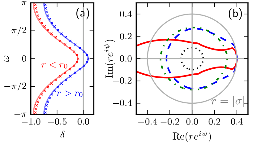
Figure 1: (Color online) (a) Pseudo-continuous spectrum $\delta(\omega)$ (lines) and location of the exact roots (crosses) for a one-dimensional complex map for $r=3.3>r_{0}=3$ and $r=2.7<r_{0}=3$. Parameters: $A=0.4$, $B=0.2$, $\psi=0$, $\tau=30$. (b) Contour line $\lambda_{\rm max}=0$ of the MSF for coupled semiconductor lasers according to Eq. (12) for delay times $\tau=1$ (solid), $8$ (dashed), $20$ (dash-dotted), and $1000$ (dotted).

Periodic orbit – Now consider the variational Eq. (2) with $A_{k}$ and $B_{k}$ being periodic in $k$ with period $T$, corresponding to a PO in the SM. We consider the case of large delay, i. e., $\tau\gg T$. Making a Floquet-like ansatz $\xi_{k}=z^{k}\,q_{k}$, where $q_{k}$ is $T$-periodic, we find

$$z\,q_{k+1}=A_{k}\,q_{k}+re^{i\psi}B_{k}\,z^{-\tau}q_{k-n}$$ (6)

with $n=\tau\,\mathrm{mod}\,T\in\{0,\,1,\dots,\,T-1\}$.

For the strongly unstable spectrum again suppose there is a solution with $|z|>1$, then in the limit $\tau\to\infty$ the term $z^{-\tau}$ vanishes and we find

$$z\,q_{k+1}=A_{k}\,q_{k}.$$ (7)

Using the periodicity of $q_{k}$, Eq. (7) implies $\det[z^{T}-\prod_{k=1}^{T}A_{k}]=0,$ where $z^{T}$ is a Floquet multiplier of the system $\xi_{k+1}=A_{k}\xi_{k}$ without delay. Hence, if $z^{T}$ is a Floquet multiplier of Eq. (7), with $|z|>1$, then in the limit $\tau\to\infty$ it is also a solution of Eq. (2) and vice versa.

For the pseudo-continuous spectrum we again make the ansatz $z=(1+\delta/\tau)e^{i\omega}$. Taking the limit $\tau\to\infty$ Eq. (6) becomes

$$e^{i\omega}\,q_{k+1}=A_{k}\,q_{k}+re^{-\delta}e^{i(\psi-\phi)}B_{k}\,q_{k-n}$$ (8)

with $\phi=\omega\tau$. Thus one has to solve

$$[e^{i\omega}\overline{J}+\overline{A}+\mu\overline{B}]\vec{q}=0,$$ (9)

where $\mu=re^{-\delta}e^{i(\psi-\phi)}$ and $\vec{q}=(q_{1},\dots,\,q_{T})$. The matrices $\overline{J}$, $\overline{A}$, and $\overline{B}$ follow from Eq. (8), taking into account the periodicity of $A_{k}$, $B_{k}$, and $q_{k}$, e.g., $\overline{A}=\mathrm{diag}\{A_{1},\dots,\,A_{T}\}$. Taking the determinant of the entire matrix in Eq. (9) results in a polynomial in $\mu=re^{-\delta}e^{i(\psi-\phi)}$ (of maximum order $Td$). Again, the roots $\mu$ are functions of $\omega$ and we can calculate the branches $\delta(\omega)=-\ln|\mu(\omega)|+\ln r$, where $\psi$ and $\phi$ drop out. As in the case of FPs, one can show that the function $|\mu(\omega)|$ is bounded $0<\mu_{0}\leq|\mu(\omega)|\leq\mu_{1}$ unless the instantaneous system has a Floquet multiplier $z$ with $|z|=1$. Note that for the FP case as well as for the PO case, one can show that the discussed strongly unstable and pseudo-continuous spectrum constitute the entire spectrum.

We have found the same structure of the MSF for a PO in the SM: The MSF is rotationally symmetric about the origin in the complex plane. If without feedback $(r=0)$ the MSF is positive, then it is a positive constant in the limit of large delay. Otherwise it is a monotonically increasing function of $r$ and it changes sign at a critical radius $r_{0}$.

Chaotic dynamics – Every chaotic attractor embeds an infinite number of unstable periodic orbits (UPOs). It is well known that the characteristic properties of the chaotic system can be described in terms of these UPOs. One of the most important examples is the natural measure of the chaotic attractor which is concentrated at the UPOs and can in fact be expressed in terms of the orbit’s Floquet multipliers GRE88 ; LAI97 .

Lyapunov exponents arising from variational equations such as Eq. (2) have been discussed in the framework of PO theory CVI95 , too. In particular it has been shown NAG97 that a chaotic attractor in an invariant manifold loses its transversal stability in a blow-out bifurcation when the transversely unstable orbits outweigh the transversely stable orbits. To be precise, we divide the orbits into these two groups and define NAG97 the transversely stable weight $\Lambda_{T}^{s}$ and the unstable weight $\Lambda_{T}^{u}$ as

$$\Lambda_{T}^{u,s} =\sum\nolimits_{j=1}^{N^{u,s}_{T}}\mu_{T}(j)\lambda_{T}(j),$$ (10)

where the sum goes over all $N^{u}_{T}$ transversely unstable and $N^{s}_{T}$ transversely stable orbits with period $T$ (or factors of $T$), respectively. Here, $\mu_{T}(j)$ is the weight of the $j$th orbit, corresponding to the natural measure of a typical trajectory in the neighborhood of the $j$th orbit and $\lambda_{T}(j)$ is the transversal Lyapunov exponent of this $j$th orbit. The weight of a PO is inversely proportional to the product of its unstable Floquet multipliers GRE88 . The attractor is transversely unstable if and only if in the limit of large $T$

$$\Lambda^{u}_{T}>|\Lambda^{s}_{T}|.$$ (11)

We now draw the connection to the scaling theory for large $\tau$. Starting from $r=0$ (no feedback), the transversal Lyapunov exponents $\lambda_{T}(j)$ of each orbit can only increase with increasing $r$, as shown above, and the weights $\mu_{T}(j)$ are not changed. In particular for large enough $r$ any orbit becomes transversely unstable: either it is already unstable for $r=0$ and thus remains unstable, or the pseudo-continuous spectrum goes to zero and for large $r$ it does so from the unstable side. Thus there exists a minimum radius $r_{0}$ for which the condition (11) on the weights is fulfilled. Note that since we consider the limit $\tau\to\infty$ we can evaluate Eq. (11) at arbitrarily large $T$. Thus in summary the MSF for chaotic dynamics has the same structure as for FPs and POs (the rotation symmetry follows from the rotation symmetry of each $\lambda_{T}(j)$).

Let us now discuss what the structure of the MSF means for the synchronizability of networks. We can classify networks into three types depending on the magnitude of the largest transversal eigenvalues $\gamma_{\rm max}$ in relation to the magnitude of the row sum $\sigma$: (a) $|\gamma_{\rm max}|<|\sigma|$, (b) $|\gamma_{\rm max}|=|\sigma|$, and (c) $|\gamma_{\rm max}|>|\sigma|$.

As we have shown above, for stable synchronization it is necessary that $|\gamma_{\rm max}|<r_{0}$. If $|\gamma_{\rm max}|>r_{0}$, the synchronization is not stable. Since $\sigma$ is the eigenvalue of the coupling matrix associated with the synchronous mode, the MSF $\lambda_{\rm max}(\sigma)$ describes the local stability within the SM, i.e., $\lambda_{\rm max}(\sigma)>0$ for chaotic dynamics in the SM and $\lambda_{\rm max}(\sigma)<0$ for FPs or POs. This implies that $|\sigma|>r_{0}$ in the first case and $|\sigma|<r_{0}$ in the latter case. In other words, the row sum $\sigma$ gives an estimate of the critical radius $r_{0}$. In particular, it allows us to give a complete classification (Table 1).

Table 1: Stability of chaotic and non-chaotic synchronized solutions for the three types of networks

	chaotic dynamics in the SM ($r_{0}<|\sigma|$)	PO or FP in the SM ($|\sigma|<r_{0}$)
(a) $|\gamma_{\rm max}|<|\sigma|$	synchr. stable if $|\gamma_{\rm max}|<r_{0}$	synchr. stable
(b) $|\gamma_{\rm max}|=|\sigma|$	synchr. unstable	synchr. stable
(c) $|\gamma_{\rm max}|>|\sigma|$	synchr. unstable	synchr. stable if $|\gamma_{\rm max}|<r_{0}$

In networks of type (a) and (b) synchronization on a FP or a PO (stable within the SM) is always stable. For type (c) this dynamics may be stable or not depending on the particular network topology (value of $|\gamma_{\rm max}|$) and the dynamics in the SM (value of $r_{0}$). On the other hand chaos synchronization is always unstable in networks of type (b) and (c) and it may be stable or not in networks of type (a) again depending on the particular network and the dynamics.

Note that, in contrast to maps, autonomous flows with a stable PO in the SM always have $r_{0}=|\sigma|$, due to the PO’s Goldstone mode. Thus for this case synchronization will be unstable for type (c) networks. For type (b) networks the stability of the synchronized solution in this case undergoes a destabilizing bifurcation.

We now list some examples for the three types of networks. The classification follows from the eigenvalue structure of the corresponding coupling matrices $g_{ij}$. Mean field coupled systems are of type (a), networks with only inhibitory or only excitatory connections are (up to the row sum factor) stochastic matrices and are thus of type (a) or (b). Rings of uni-directionally coupled elements and two bidirectionally coupled elements are of type (b) and any network with zero row sum ($\sigma=0$) is of type (b) (trivial case) or (c) and therefore these systems can never exhibit chaos synchronization.

Another conclusion we can draw from the structure of the MSF confirms the conjecture stated in KIN09 : networks with $\sigma=0$ are of type (c) and thus chaos synchronization is always unstable.

Concerning the impact of noise on the delay-coupled network HUN10 , for the case of FPs and POs stable synchronization will be robust to small noise strength. On the other hand, for the chaotic case there may exist another radius $r_{b}<r_{0}$, where the first UPO in the attractor loses its transverse stability and the attractor undergoes a bubbling bifurcation OTT94 ; ASH96a . Then any network with $r_{b}<|\gamma_{\rm max}|<r_{0}$ will exhibit bubbling in the presence of small noise (or parameter mismatch), while any network with $|\gamma_{\rm max}|<r_{b}$ will show stable synchronization, even in the presence of small noise. For large noise strength the linear theory cannot make predictions.

Example – As an example we consider a network of optically coupled semiconductor lasers modeled by dimensionless equations of Lang-Kobayashi LAN80b type

$$\dot{E}^{l}(t) ={\textstyle\frac{1}{2}}(1+i\alpha)\,n^{l}(t)\,E^{l}(t)+\sum\nolimits_{j=1}^{N}g_{lj}\,E^{j}(t-\tau),$$

$$T\,\dot{n}^{l}(t) =p-n^{l}(t)-\left(1+n^{l}(t)\right)|E^{l}(t)|^{2},$$ (12)

where $E^{l}$ and $n^{l}$ are the complex electric field amplitude and the inversion of the $l$-th laser, respectively. For our example, we choose the parameters as follows: Ratio between carrier and photon lifetime $T=200$, injection current $p=10$, $\alpha$-factor $\alpha=4$. This results in a relaxation oscillation period $T_{RO}\approx 28$. Figure 1b shows the $\lambda_{\rm max}=0$ contour line of the corresponding MSF for networks with $\sigma=0.4$ for different values of the delay time $\tau$. For $\tau=20$ (order of $T_{RO}$) the contour line starts to become circular. For $\tau\gtrsim 3T_{RO}$ the shape of the MSF perfectly resembles our predictions. In this case we find $r_{0}<\sigma=0.4$, i. e., the dynamics is chaotic. For $\tau=1$ and $10$ the limit of large delay is not satisfied, hence the MSF does not exhibit the rotation symmetry. Note that for these values of the delay time the dynamics is a PO and since the system is a flow, the stability boundary reaches its maximum real value at $re^{i\psi}=|\sigma|$.

Conclusion – We have shown that the MSF has a simple universal structure in the limit of large delay: it is rotationally symmetric around the origin and either positive and constant (if it is positive at the origin), or monotonically increasing and becoming positive at a critical radius $r_{0}$. This structure allows us to confirm a recent conjecture KIN09 about synchronizability of chaotic elements. Furthermore, we classify networks into three types depending on the magnitude of the maximum transversal eigenvalue of the coupling matrix in relation to the magnitude of the row sum. Importantly, this classification allows us to predict the synchronizability of general networks of identical units with strongly delayed connections based solely on the modulus of the eigenvalues and the type of synchronized dynamics. In many cases this prediction is possible even without computing the critical radius $r_{0}$ (as shown in Table I). Although our results describe the properties of coupled systems in the limit of large delay, practically they are expected to hold when the delay is two or three times larger than the characteristic timescale of the underlying system without delay. This is confirmed by our example as well as the results of Refs. FAR82GIA96MEN98WOL06YAN06YAN09 .

This work was supported by DFG (Sfb 555 and Research Center MATHEON under project D21).

References

- (1) A. S. Pikovsky et al., Synchronization, A Universal Concept in Nonlinear Sciences (Cambridge University Press, Cambridge, 2001).
- (2) K. M. Cuomo and A. V. Oppenheim, Phys. Rev. Lett. 71, 65 (1993); S. Boccaletti et al., Phys. Rep. 366, 1 (2002); I. Kanter et al., Phys. Rev. Lett. 101, 84102 (2008);
- (3) W. Singer, Neuron 24, 49 (1999).
- (4) P. A. Tass et al., Phys. Rev. Lett. 81, 3291 (1998).
- (5) H. J. Wünsche et al., Phys. Rev. Lett. 94, 163901 (2005); T. W. Carr et al., SIAM J. Appl. Dyn. Syst. 5, 699 (2006); H. Erzgräber et al., SIAM J. Appl. Dyn. Syst. 5, 30 (2006); I. Fischer et al., Phys. Rev. Lett. 97, 123902 (2006); O. D’Huys et al., Chaos 18, 037116 (2008).
- (6) E. Rossoni et al., Phys. Rev. E 71, 061904 (2005); C. Masoller et al., Phys. Rev. E 78, 041907 (2008).
- (7) A. Takamatsu et al., Phys. Rev. Lett. 87, 078102 (2001).
- (8) L. M. Pecora and T. L. Carroll, Phys. Rev. Lett. 80, 2109 (1998).
- (9) M. Dhamala et al., Phys. Rev. Lett. 92, 074104 (2004); C.-U. Choe et al., Phys. Rev. E 81, 025205(R) (2010).
- (10) W. Kinzel et al., Phys. Rev. E 79, 056207 (2009).
- (11) J. D. Farmer, Physica D 4, 366 (1982); G. Giacomelli and A. Politi, Phys. Rev. Lett. 76, 2686 (1996); B. Mensour and A. Longtin, Physica D 113, 1 (1998); M. Wolfrum and S. Yanchuk, Phys. Rev. Lett. 96, 220201 (2006); S. Yanchuk et al., Phys. Rev. E 74, 026201 (2006); S. Yanchuk and P. Perlikowski, Phys. Rev. E 79, 046221 (2009).
- (12) C. Grebogi et al., Phys. Rev. A 37, 1711 (1988).
- (13) Y. C. Lai et al., Phys. Rev. Lett. 79, 649 (1997).
- (14) P. Cvitanović, Physica D 83, 109 (1995).
- (15) Y. Nagai and Y. C. Lai, Phys. Rev. E 56, 4031 (1997).
- (16) D. Hunt et al., Phys. Rev. Lett. 105, 068701 (2010).
- (17) E. Ott and J. C. Sommerer, Phys. Lett. A 188, 39 (1994).
- (18) P. Ashwin et al., Nonlinearity 9, 703 (1996).
- (19) R. Lang and K. Kobayashi, IEEE J. Quantum Electron. 16, 347 (1980).